Abstract
Pulsed thermography is commonly used as a non-destructive technique for evaluating defects within materials and components. In the last few years, many algorithms have been developed with the aim to detect defects and different methods have been used for detecting their size and depth. However, only few works in the literature reported a comparison among the different algorithms in terms of the number of detected defects, the time spent in testing and analysis, and the quantitative evaluation of size and depth. In this work, starting from a pulsed thermographic test carried out on an aluminum specimen with twenty flat bottom holes of known nominal size and depth, different algorithms have been used with the aim to obtain a comparison among them in terms of signal to background contrast (SBC) and number of detected defects by analyzing different time intervals. Moreover, the correlation between SBC and the aspect ratio of the defects has been investigated. The algorithms used have been: Pulsed Phase Thermography (PPT), Slope, Correlation Coefficient (R2), Thermal Signal Reconstruction (TSR) and Principal Component Thermography (PCT). The results showed the advantages, disadvantages, and sensitivity of the various thermographic algorithms.
1. Introduction
Aluminum alloys, thanks to their low density and ability to resist corrosion, are widely used for manufacturing mechanical components and large structures and, in this regard, many examples can be found in different engineering fields from building to automotive and aerospace.
During the manufacturing processes or in-service conditions, several defects may appear in materials that can affect the structure and its mechanical properties. Therefore, it is very important to check the integrity of the components to reveal these defects.
Several non-destructive techniques (NDT) can be used to detect such defects such as X-ray, ultrasound [1], eddy current [2], magnetic method [3] and penetrant test.
Wilczek et al. [1] performed a comparison among different NDT techniques such as: X-ray, ultrasonic, eddy current and thermography to detect flaws in aluminum pressure die casting. Regarding the porosity detection in aluminum pressure die casting, the radiographic method allows for analyzing raw casting without surface preparation while eddy current and thermography are not suitable for the detection of fine porosity.
In the work of Postolache et al. [2] a system architecture based on the eddy current method has been used to detect cracks on aluminum aircraft plates. In particular, superficial and sub-superficial cracks were detected by adopting image filtering techniques based on a 2D stationary wavelet transform, Wiener linear filtering and soft-thresholding.
A non-destructive testing method for thin-plate aluminum alloys based on the geomagnetic field has been proposed in the work of Hu et al. [3]. This method allows for detecting the artificial groove and natural defects in thin-plate with a thickness of less than 2 mm.
In the case of large structures, it is required a rapid and easy inspection of the components in order to reduce the time of the ordinary maintenance and thus to limit the costs. In this regard, it is very important to develop automatic procedures and algorithms for data analysis to obtain very quickly, the quantitative characterization of defects.
Stimulated thermography [4,5,6,7,8] presents the peculiarities suitable for investigation of large areas since it does not require the coupling with the component, is easily automatable and the testing time is relatively short with respect to other traditional well-established NDT techniques. Different thermographic techniques (Pulsed and Lock-in) [4,5,6,7,8] and heat sources can be used to detect defects in large aluminum components.
Oswald-Tranta [9,10] demonstrated in her works that inductive pulse and lock-in thermography are capable in evaluating surface cracks also on non-magnetic materials such as aluminum. In particular, the lock-in approach improves the signal to noise ratio since a sequence of short pulses is applied. With the aim to detect similar defects, laser spot thermography and vibrothermography techniques were used in the work of Roemer et al. [11]. In the paper, the effectiveness of the two presented methods has been demonstrated in evaluating very small defects.
In the work of Maldague et al. [12] several defects were considered for the inspection of aluminum specimens by transient infrared thermography. Authors highlight as flash tubes with heat pulse energy of about 5–20 kJ are sufficient to thermally stimulate the material and a high frame rate is needed to better resolve the thermal process.
In the literature, authors focus their attention on the signal to noise ratio or signal to background contrast, neglecting the influence of the number of analyzed frames on this quantitative parameter. Hence, in this work, a comparison among different algorithms used for processing thermal data derived from a Pulsed thermographic test is provided with the aim of highlighting the strong and weak points of each algorithm in terms of signal to background contrast (SBC), number of detected defects, and the influence of the number of analyzed frames. Another important aim of this work is to demonstrate as a good correlation between two different parameters, the SBC and the aspect ratio r (diameter/depth), for estimating the size and the depth of defects.
The Pulsed Thermography (PT) technique has been applied on an aluminum specimen with flat bottom holes to simulate the presence of defects. Several algorithms have been implemented to elaborate raw thermal data: Pulsed Phase Thermography (PPT) [12,13,14,15,16,17], Thermal Signal Reconstruction (TSR) [18,19,20,21,22,23,24], Principal Component Thermography (PCT) [25,26,27,28,29,30], Slope and Correlation coefficient (R2) [31,32].
Results show as each algorithm has its own peculiarities and capabilities and a synergic action in defects detection and characterization can be obtained if more algorithms are applied on the same thermal sequence.
2. Theory: Pulsed Thermography
The basic approach of the active/stimulated thermography is based on inducing thermal waves within the specimen by means of an external heat source and monitoring the superficial temperature changes. In literature, there are three classical active/stimulated thermography techniques that differ for the heating source modulation: Pulsed Thermography (PT), Lock-in Thermography (LT) and Stepped Heating Thermography (SHT) [4]. In each case, thermographic raw data provide few information about the presence of defects because of the low value of the signal to noise ratio. In this regard, a post-processing analysis is necessary to improve the quality of the results by means of different algorithms.
In this work, the PT technique has been used, and different post-processing algorithms were compared, starting from the same thermal sequence.
The PT technique consists of a short heat impulse using a power heating source. The presence of subsurface discontinues changes in the diffusion of heat flow and produces a change of cooling over time.
The one-dimensional solution of the Fourier’s Law for a Dirac delta heating pulse propagation through a semi-infinite homogeneous material is given by this following equation:
where Q is the energy absorbed by the surface; T0 is the initial temperature; α is the thermal diffusivity and e is the effusivity.
Considering the temperature evolution of the inspected surface, Equation (1) can be rewritten as (z = 0):
That means a constant cooling slope of value 0.5 in log-log scale [4,5,6,7,8,9,10,11,12,13,14,15,16,17,18,19,20,21,22,23,24,25,26,27,28,29,30,31,32]. In the presence of a defect, Equations (1) and (2) are not valid anymore and a change in slope can be observed due to a different diffusion of thermal waves within the specimen.
Data acquisition in PT is fast and allows the inspection of wide area surfaces. However, as already said, raw PT data are difficult to analyze because of non-uniform heating or reflections. In the next paragraphs, the pre- and post-processing algorithms used to detect defects will be discussed in detail.
2.1. Post-Processing Algorithms: Pulsed Phase Thermography (PPT)
Pulsed phase thermography (PPT) [12,13,14,15,16,17] is a technique that transforms thermographic data from the time domain into the frequency domain using Fast Fourier Transform (FFT).
Any wave form, periodic or not, can be approximated by the sum of purely harmonic waves oscillating at different frequencies. The Continuous Fourier Transform (CFT) can be expressed as:
where . For the PPT the Discrete Fourier Transform (DFT) is used working with PT data:
where Re and Im are respectively the real part and imaginary part of the transformed data, the subscript n is the increasing frequency, ∆t is the sampling interval; N is the total number of thermograms (infrared images). The phase and amplitude maps are finally obtained using the following relation:
Amplitude and phase maps (Figure 1) are obtained by repeating this process for all pixels (x, y) of the field of view. With N time increments available (with N corresponds also to the thermograms in the sequence), N/2 frequency values are available (due to the symmetry of the Fourier transforms [4].
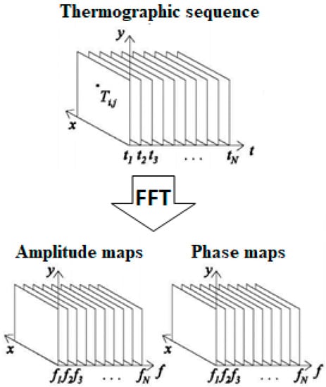
Figure 1.
Data acquisition and processing by Pulsed Phase Thermography (PPT).
The quality of the results depends on two important parameters, the sampling rate fs, and the acquisition time (tacq); i.e., the maximum truncation window w(t).
Theoretically, the sampling rate should be high enough to increase the available frequency (fmax = fs/2) and capture early thermal changes.
The truncation window w(t) should be as large as possible to increase frequency resolution and to be able to characterize a wide range of depths, especially deep defects that are detectable only at very low frequencies.
The material thermal properties are critical in the choosing of Δt and w(t). In fact, the much higher time resolution requirement on high conductivity materials is compensated in part by the need of a smaller truncation window. More frames had to be included for the aluminum to incorporate more data, especially at the beginning of the sequence, where thermal changes are critical. The number of frames N could be further reduced without loss of pertinent information using a higher sampling rate with a shorter w(t) [15].
Other details about the testing parameters for the PPT technique can be found in references [17,18,19,20,21,22,23,24,25,26,27,28,29,30,31,32].
The Fast Fourier Transform (FFT) algorithm, available in software packages such as MatLab®, greatly reduces the computation time and is therefore privileged. It should also be pointed out that the direct implementation of the DFT, as shown in Equation (3) above, requires approximately n2 complex operations. However, computationally efficient algorithms can require as little as n log2(n) operations.
2.2. Post-Processing Algorithms: Thermal Signal Reconstruction (TSR)
Thermographic signal reconstruction (TSR) [18,19,20,21,22,23,24] assumes that temperature profiles for non-defective pixels should follow the decay curve given by the 1D solution of the Dirac equation, Equation (2), which may be rewritten in the logarithmic form as:
which corresponds to a straight line with slope −0.5 in a double ln scale, as shown in Figure 2.
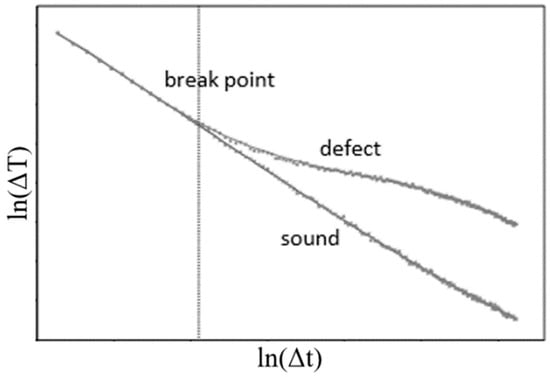
Figure 2.
Trend of cooling curve in a double logarithmic scale.
In presence of defects, Equation (6) is no longer valid and a deviation of the cooling curve from sound material can be observed. In this case, the cooling curve can be fitted in the logarithmic domain by means of a polynomial function (Equation (7)). It has been found that a 5th (or 7th order) polynomial provides an excellent fit to PT data since the inclusion of higher order terms only replicates noise. As can be observed in Equation (7), one of the main steps in the regression process in TSR is the selection of the appropriate number of coefficients n to fit the thermographic data. For isotropic materials, a good correspondence between acquired data and fitted values can be achieved by setting n to 4 or 5, given the number of inflection points of the thermal profiles.
As a result, the TSR method (Figure 3) provides a significant degree of data compression; in fact, there is a replacement of the sequence of temperature maps in time, by a series of (n + 1) images that correspond to the polynomial coefficient: ao(i,j),…, an(i,j). From this series of (n + 1) maps it is possible to reconstruct a full thermographic sequence. In addition, it is possible to obtain a drastic reduction of the data amount. It is also convenient to analyze the 1st and the 2nd logarithmic derivatives of the thermographic sequence, which derive directly on the polynomial [19]. With this fitting operation there is a significant reduction of the original temporal noise and the transition to the derivative analysis increases the contrast between the defective and the relative sound area. For each pixel, the time sequence can be differentiated using these expressions:
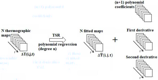
Figure 3.
Defect detection by the Thermal Signal Reconstruction (TSR) method, logarithmic derivation.
The selection of experimental parameters is more intuitive than for the PPT: for high conductivity materials and shallow defects it is necessary to choose a high sampling frequency and short acquisition time because the time evolution of the surface temperature changes rapidly; for low conductivity materials and deep defects it is better to choose a low sampling frequency and a long acquisition time since the time evolution of the surface temperature changes slowly.
2.3. Post-Processing Algorithms: Principal Component Thermography (PCT)
PCT is a thermographic algorithm based on the Principal Component Analysis (PCA) to extract features and reduce the noise by projecting the thermal response data into a system of orthogonal components [25,26,27,28,29,30]. In general, the PCA is a linear projection technique for converting a matrix A to a matrix of the lower dimension by projecting A into a new set of principal axes. One simple approach to the PCA is to use Singular Value Decomposition (SVD), already implemented in the software Matlab as a function. In general, a matrix A of the dimension M × N (M > N) can be decomposed as:
where U is the eigenvector matrix of the dimension M × N, R is an N × N diagonal matrix with positive or zero elements representing the singular values of matrix A, and VT is the transpose of an N × N matrix.
To apply the SVD to thermographic data, the 3D thermogram matrix representing time and spatial variations has to be converted in a 2D M × N matrix A [29,30]. This can be done by converting the thermograms for each time as columns in A, as illustrated in Figure 4 [21]. Under this configuration, the columns of U represent a set of orthogonal statistical modes known as Empirical Orthogonal Functions (EOFs) that describe the data spatial variations. Besides, the Principal Components (PCs), which represent time variations, are arranged in matrix VT. The resulting U matrix that provide spatial information can be reconverted into a 3D sequence as illustrated in Figure 4 [30].
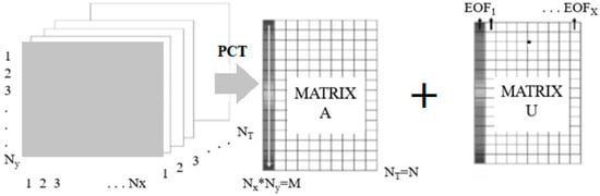
Figure 4.
Thermographic data conversion from a 3D sequence to a 2D A matrix in order to apply Singular Value Decomposition (SVD) and finally conversion of 2D U matrix into a 3D matrix containing the Empirical Orthogonal Functions (EOFs).
The uncorrelated variables are linear combinations of the original variables, and the first component contain the data with higher variance, while the consecutive components are with decreasing variances, so they are a symbol of noise. Therefore, only few components, in particular the second principal component, need to be examined in the thermography data analysis to detect defects.
2.4. Post-Processing Algorithms: Slope and R2
Two parameters have been used to analyze thermal data during the cooling phase of the Pulsed Thermography test: the slope (m) and the linearity R2 (T-R2 module) of data [31,32]. In fact, the presence of the defect determines a modification of thermal profile during cooling with a typical non-linear behavior. In the case of a simple linear regression, R2 equals the square of the Pearson correlation coefficient between the observed and predicted data values of the dependent variable [31].
3. Materials and Methods
3.1. Materials and Experimental Set-Up
An aluminum sample, shown in Figure 5, with 20 flat bottom holes of different diameters and depths has been tested with one pulsed test.
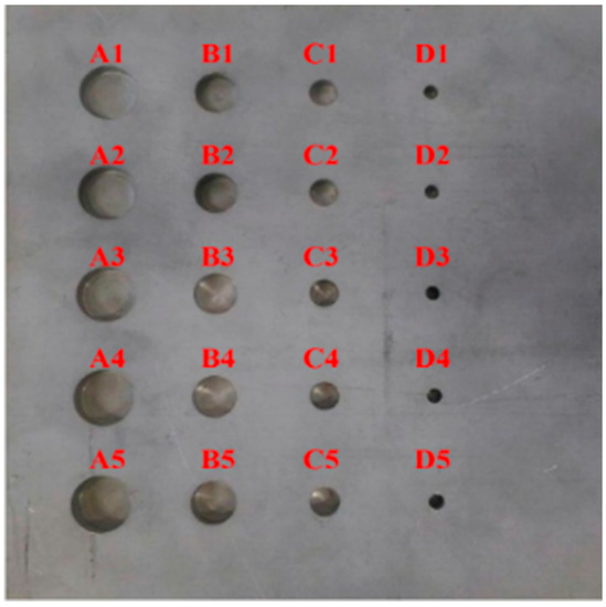
Figure 5.
Aluminum sample with simulated defects used for tests.
The different sizes and depths of simulated defects are reported in Table 1:

Table 1.
Flat-bottom holes sizes and depths of the tested sample.
A pulsed thermography test was performed using the IR camera FLIR X6540 SC (FLIR Systems Inc., Wilsonville, OR, USA) with thermal sensitivity (NETD) <25 mK and based on a cooled detector with 640 × 512 pixels. The used set-up is shown in Figure 6. In particular, two flash laps with a total energy of 3000 J were positioned very close to the specimen (10 cm) and at the same side of the IR camera (angle 45°). This latter was placed at about 1 m from the specimen in order to obtain a geometrical resolution of 0.25 mm/pixel. The two lamps are synchronized using the same power generator.
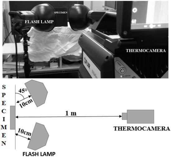
Figure 6.
Set-up used for pulsed thermography test.
The thermal sequence was acquired with a sample rate of 200 Hz, with an observation time of 10 s. It is important to underline as 200 Hz represents the maximum value of the sample rate obtainable from the IR camera to obtain the full frame of the whole specimen. Moreover, three replicates of the same test were carried out, maintaining unaltered set-ups and test parameters.
3.2. Processing of Thermographic Data
The algorithms described in Section 2 were computed by using the MATLAB® software with the aim to obtain quantitative information from the acquired data. In particular, seven different sets of frames and then seven intervals of the cooling curve were chosen for analysis: 16, 32, 64, 128, 256, 512, and 1024 frames [33]. The power of two for each interval has been chosen to perform a fast post processing analysis with the PPT algorithm (Fast Fourier Transform). The last interval corresponds to 5.12 s. The starting frame for all analysis intervals is the same and it corresponds to the ΔTmax value, pixel by pixel. The sampling rate for all analysis intervals is the same and it is equal to 200 Hz.
A pre-processing procedure was implemented before the application of each algorithm. The steps of this procedure can be summarized as follows:
- Importing of the thermographic sequence (3D matrix);
- Subtracting of the average of the first ten cold frames to the whole sequence to obtain the ΔT values over time;
- Adding an offset value to the pixels in the frames where a negative ΔT value is reached. These pixels occur in the last frames of the sequence and represent a small part of the frame. Hence, they do not affect normalization; this step evaluates ΔT values in the logarithmic scale.
- Normalising the local temperature values at any time by dividing them to the value evaluated at time t’ sufficiently near to the pulse occurrence (the time t’ corresponds to the instant in which the maximum ΔT is reached) [19].
The advantage of this step is to reduce the effects of non-perfect heating of the sample and the variability of the optical properties of the surface, such as absorptivity and emissivity [6].
- The 3D final temperature matrix is divided in seven intervals over time in order to process the data with the proposed algorithms.
Each algorithm was implemented by using the various functions already present in the Matlab library. More precisely:
- -
- The fft function for the PPT algorithm and the angle and the abs functions to obtain the phase and the amplitude maps, respectively;
- -
- The svd function for the PCT algorithm;
- -
- The polifyt, polyval and polyder functions for the TSR (5°), Slope and R2 algorithms.
These functions are been applied on the normalized delta-temperature signal, without the necessity to modify the guidelines indicated in the Matlab help. In particular, by using the fft function already implemented in Matlab environment, the discrete Fourier transform (DFT) of the signal is computed, pixel by pixel, using a fast Fourier transform (FFT) algorithm, already written in Matlab. In this way, the signal is obtained for each pixel along the frequency spectrum and, using the angle and abs functions, the amplitude and the phase maps are computed for each analyzed frequency. Obviously, the obtained results in terms of phase and amplitude depend on the truncation window size (analysis interval) and on the acquisition frequency.
For the PCT algorithm, the svd function in Matlab returns numeric unitary matrices U and V with the columns containing the singular vectors, and a diagonal matrix S containing the singular values. The matrices satisfy the condition A = U × S × V’, where A is the initial matrix with the normalized delta-temperature, pixrl by pixel, and where V’ is the Hermitian transpose (the complex conjugate of the transpose) of V. The singular vector computation uses variable-precision arithmetic. In this case, the economical svd version has been chosen because it is faster: if A is an m-by-n matrix with m > n, then svd computes only the first n columns of U. In particular, the matrix U contains the principal components, used to achieve the results shown.
The evaluation of slope, R2 and 1st and 2nd derivatives (TSR algorithm) has been obtained by processing the thermal sequences using the Matlab commands polifyt, polyval and polyder for a polynomial fit of the data of degree 1 in the case of slope and R2 and 5 for 1st and 2nd derivatives. In order to evaluate the polynomial coefficients, the already implemented Matlab functions perform an ordinary least squares calculation.
The signal contrast, expressed as the signal-to-noise ratio, was chosen as a term of comparison between the different algorithms.
The most used definition of the thermal contrast is the Absolute Thermal Contrast, which measures the difference between defective and sound zones [34,35]:
where T is the temperature signal, t is the time variable, and the subscripts d and s refer to the defective and sound areas, respectively.
Typically, a sound region can be identified either automatically or by an operator, and then Ca is computed. Ca is dependent on the absorbed energy, and then a different definition is necessary to improve the capability of a defect detection. Running contrast is less affected by the surface optical properties and it depends less on the energy absorbed. It is defined as:
In this work, the Signal to Background Contrast (SBC) was introduced for defects characterization. The SBC is similar to the well-known Signal to Noise Ratio (SNR) and is expressed as [34]:
where MSD is the signal due to the defect, MSS is the mean value of the sound and SDS is the standard deviation of the sound (background).
In Figure 7, a typical signal trend is shown along a profile taken on the first row of defects. The signal plot refers to the amplitude data obtained with the PPT algorithm with 512 frames.
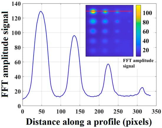
Figure 7.
An example of the amplitude signal (PPT) along a profile in which are highlighted the peaks of the signal due to the first row of defects; (0.3906 Hz with 512 analyzed frames).
In correspondence of the signal peak of each defect, the average value of a 3 × 3 matrix was taken to assess the MSD value. In Figure 8 the sound areas chosen to assess the MSS and SDS values are shown. For each defect, the same sound area has been considered as the sum of the sound areas indicated in red in Figure 8.
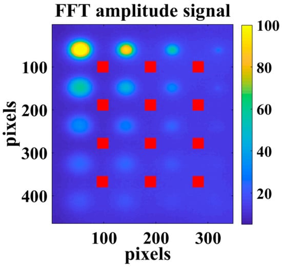
Figure 8.
An example of the obtained thermographic map (PPT, amplitude) with in red the areas chosen as sound; (0.3906 Hz with 512 analyzed frames).
4. Results
4.1. Preliminary Analysis
The aim of this work is to compare different algorithms in terms of the capacity to detect a defect. This capacity has been evaluated by considering two different parameters:
- number of detected defects;
- maximum SBC;
The defect detection has been assessed by imposing a threshold value equal to two times the SDS, for each of the seven intervals chosen for analysis. In this way, defects are detected if:
In the literature, a similar criterion has been used for the quantitative analysis of defects [35]. It is important to underline as the threshold value depends on several factors such as, the material, kind of defects, adopted heat sources, surface condition, etc. In our case, as shown in Figure 9, in which it is reported the case of the slope algorithm with 1024 frames, the chosen threshold seems to give a good response about the detectability of defects. In fact, the threshold value allows for detecting at least the defects above the aspect ratio of two, which represents the limit for the PT technique [4,15] and discards the false positives. Moreover, the proposed approach follows the probabilistic criterion according to which, if a phenomenon is distributed as a gaussian normal distribution, the 95% of the values falls in the range between . It follows that the probability of finding a single defected pixel with a contrast below is equal to 0.025. As exposed in the previous section, in this work, an indication is considered a defect only if there is at least a set of nearby pixels equal to 9 (as MSD a matrix equal to 3 × 3 has been chosen). In this case, the probability is even lower since it for 9 single pixels drops to 7.63 × 10⁻¹⁵.
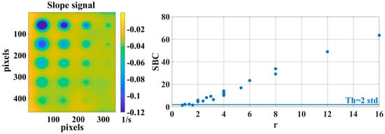
Figure 9.
The Signal to Background Contrast (SBC) trend versus the ratio r in the case of slope algorithm by computing 1024 frames; the influence of the threshold value on the defect detectability.
4.2. Comparison of the Different Algorithms in Terms of SBC
The Figure 10 shows the trend of the maximum SBC versus the aspect ratio r for each algorithm independently by the frame interval at which this is achieved.

Figure 10.
Comparison of different algorithms in terms of maximum SBC.
As expected, the SBC is influenced by the aspect ratio r and in this regard, it is not simple to discern the best algorithm by considering only the maximum value of the SBC. In fact, for the defects with a small ratio r < 4, the TSR analysis returns a 2nd derivative that seems to get the better results; the PCT and the 1st derivative show a higher SBC with respect to the 2nd derivative for the larger and superficial defects. The PPT algorithm, both for the amplitude and the phase, seems to show the lower SBC value for most of the detected defects. Finally, the R2 algorithm seems to be “in the middle” of the achieved results.
To obtain a parameter able to quantify the goodness of each algorithm in terms of the maximum SBC value, the weighted average has been calculated as follows (Table 2):
when xi indicates the SBC value for each defect and pi is the relative weight, represented by the aspect ratio r; the defects below the threshold value were considered with SBC equal to 0.
Table 2.
The maximum SBC value for each algorithm obtained with Equation (15).
The results reported in the Table 2 confirm the comments that emerged from the previous graphical comparison; it seems that the PCT returns better results.
4.3. Comparison of the Different Algorithms in Terms of the Number of Detected Defects
Another way to compare the different algorithms consists on the analysis of the number of the detected defects for each interval. The obtained results are presented in a bar plot (Figure 11) by reporting in x-axis the different chosen intervals and in y-axis the number of the detected defects for each algorithm. The same results obtained in [34] are confirmed, where only R2, slope and phase PPT algorithms were compared: the analysis of the results deriving from R2 algorithm allows for detecting the greatest number of defects equal to 19/20 by analyzing only 32 frames. The same results are obtained in the case of a TSR analysis with the 2nd derivative and PCT analysis with the 2nd principal component. In this case, a higher number of frames equal to 512 for the TSR case and 1024 for the PCT case is requested, and so a more computational time is necessary in both cases.
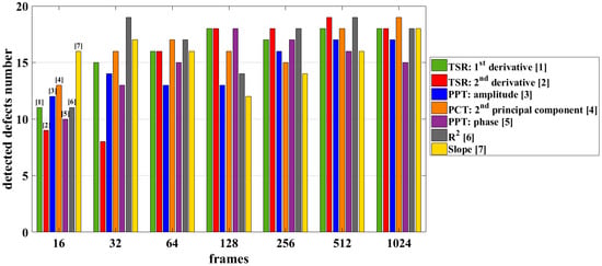
Figure 11.
Comparison among the different algorithms in terms of the detected defects number for each interval in a bar plot.
In Section 4.5, the maps corresponding with the better analysis interval in terms of the greatest detected defects number will be reported.
4.4. Comparison of the Different Algorithms: Correlation between SBC and r
The final comparison regards the possibility to obtain a good correlation between the SBC and the size of the detected defects, which are expressed in terms of the aspect ratio r. In this case, the linear correlation has been taken into account and the square of the correlation coefficient has been considered to evaluate the goodness of the correlation.
For example, in Figure 12, several trends for each analyzed interval are shown in the case of the Slope algorithm.
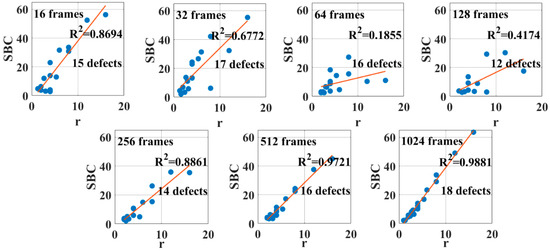
Figure 12.
SBC values for the Slope algorithm and for different frame intervals.
For completeness of information, in Figure 12, the goodness of fit expressed by comparison R2 and the number of detected defects is reported, using the same scale. In Table 3, the obtained results for each interval are summarized.
Table 3.
Slope algorithm: Evaluation of the SBC-r correlation for different frame intervals.
In this case, for this algorithm, the better results, in terms of both the linearity and the number of detected defects, are obtained for a number of frames equal to 1024. This is not always true in the case of the other algorithms and not always a good correlation between SBC and how r is obtained.
For brevity, in the Figure 13, Figure 14, Figure 15, Figure 16, Figure 17, Figure 18 and Figure 19, the better results in terms of linearity between SBC and r for each algorithm are shown, regardless the number of the analyzed frames.
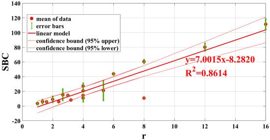
Figure 13.
SBC versus r for TSR 1st derivative 1024 frames, error bars and confidence bounds on the find linear model.
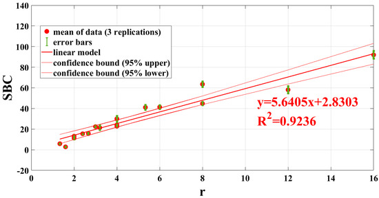
Figure 14.
SBC versus r for TSR 2nd derivative 256 frames, error bands and confidence bounds on the find linear model.
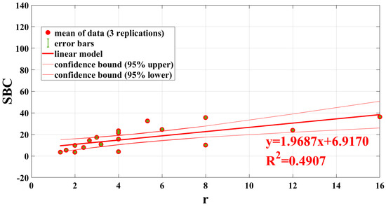
Figure 15.
SBC versus r for PPT (phase) 128 frames, error bands and confidence bounds on the find linear model.
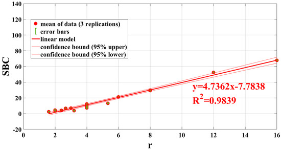
Figure 16.
SBC versus r for PPT (amplitude) 512 frames (0.3906 Hz), error bands and confidence bounds on the find linear model.
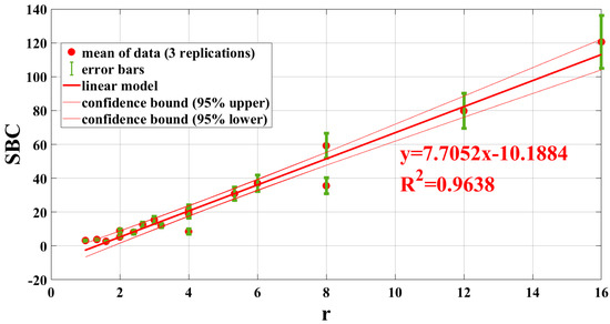
Figure 17.
SBC versus r for PCT (2nd principal component) 1024 frames, error bands and confidence bounds on the find linear model.
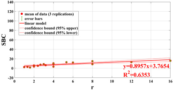
Figure 18.
SBC versus r for R2 512 frames, error bands and confidence bounds on the find linear model.
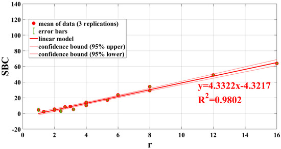
Figure 19.
SBC versus r for slope 1024 frames, error bands and confidence bounds on the find linear model.
In Table 4, the obtained results for each algorithm are summarized:
Table 4.
Comparison among the different algorithms in terms of the linear correlation between SBC and r.
From Table 4, it emerges that the algorithm of the PPT amplitude returns the better results, with a value of a square correlation coefficient equal to 0.98. On the contrary, it seems that the worst algorithm is the PPT phase, because for this algorithm the SBC is less influenced by the value of the aspect ratio r (Figure 15).
For each algorithm, a linear correlation between the SBC trend and r has been found and so the presence of a possible model between these two parameters has been highlighted. For completeness of information, in the Figure 13, Figure 14, Figure 15, Figure 16, Figure 17, Figure 18 and Figure 19, the error bar has been reported for each detected defect and for each aspect ratio. The error bar has to be considered as the standard deviation of the single data from the average of three replications. Besides, for each found linear model the confidence bounds at 95% are reported.
From the analysis of these statistical parameters, different results emerge; in particular, from the analysis of the error bars, the PCT algorithm seems to return very different contrast values, and so the results of the application of this algorithm seem to be non-repeatable. It is noteworthy that the reported error is not a measurement error but an error on the obtained results in terms of contrast.
Instead, for the linear model and the relative confidence bounds at 95%, the algorithms of the R2, slope and amplitude return the better results, because the width of the confidence interval is very narrow, and thus the data are distributed very well around the chosen model.
4.4.1. Quantitative Analysis: The Proposed Procedure Based on the Correlation between the SBC and the Aspect Ratio r
In this paragraph, a first attempt of estimating the size and the depth of the defect, by using the correlation between the amplitude SBC and the aspect ratio r, is reported. The considered results are those deriving from the amplitude (PPT) because the square correlation coefficient is the highest. In particular, a defect with an aspect ratio equal to six has been eliminated from the obtained results to use it as validation of the method. The size of this defect is estimated with a well-established method [33]: the contrast between the defect and the sound is evaluated as explained in Section 3.2 and a threshold equal to half of this value is chosen to discern defect and sound pixels. In Figure 20, the passage between the amplitude map and its binarized map (1 defect 0 sound) is shown.
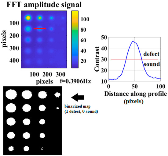
Figure 20.
Estimation of defect size with the semi-contrast method [33] (PPT amplitude, 0.3906 Hz with 512 frames).
The measure of the defect size, highlighted in red in the Figure 20, is equal to 12.59 mm by knowing the ratio mm/pixel.
By using the relative correlation between the SBC and the aspect ratio r, obtained by considering the same defects of Figure 16 (except the defect for the validation of the method) and reversing the axes, it is possible to enter in this plot the SBC value of the defect and to obtain the relative r with the equation reported in Figure 21. If the size of the defect, calculated by the semi-contrast method or similar methods, is known, it is possible to evaluate the depth of the defect that in this case is equal to 2.05 mm. In Table 5, an estimation of the error committed by evaluating the size and the depth of the defect in this way is reported:
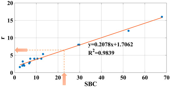
Figure 21.
Calibration curve, (PPT amplitude, 0.3906 Hz with 512 frames).
Table 5.
Estimation error in evaluating the size and the depth of the defect with the amplitude algorithm (PPT).
As it is possible to observe from the results reported in Table 5 that the estimation of the size and the depth of the defect is very good, the errors with respect to the nominal values are in fact very little.
A broader comparison among the estimation and the relative errors obtained by using the different algorithms and the methods already used in the literature for this aim (peak 2nd derivative time in TSR and the so-called blind frequency in PPT) [36,37] will be exposed in the subsequent work.
4.5. Comparison of Different Algorithms in Terms of Maximum SBC, Number of Detected Defects and the Correlation SBC vs. r
In this section, the obtained results are summarized and the algorithms are compared in terms of maximum SBC, number of detected defects and the correlation of SBC vs. r.
In Figure 22, the results, as 2D maps, are represented for each algorithm. In particular, each of them represents the map in which the greatest number of defects is detected, also as illustrated in the bar plot in Figure 11. For some of the analyzed algorithms (TSR and PPT), there is more than one frame interval in which the greatest number of defects is detected. In this case, the map corresponding to the smaller interval is shown for each algorithm. Moreover, in Figure 22, the maps of the TSR and PPT algorithms have been obtained by considering, for each defect, the time (TSR) and the frequency (PPT) in which the SBC max is reached.
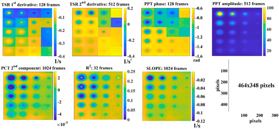
Figure 22.
Best maps for each algorithm and for the intervals for which the greatest number of defects were detected.
In Table 6, the obtained results are summarized. The better results are highlighted in bold. In particular, columns 2 and 3 refer respectively to the number of frames obtained for the best linearity and the maximum number of detected defects.
Table 6.
Final comparison among the different algorithms.
In italic, a good compromise result is highlighted. The greatest number of defects, equal to 19/20, is detected by the application of the PCT algorithm with a good correlation (linearity) in the correspondence of 1024 frames. In addition, the PCT algorithm returns the maximum SBC, as indicated in Table 2.
5. Discussion
In the literature, there are several works that show a comparison among the different thermographic techniques and algorithms [4] in terms of the capability to detect a defect [32,33,34,35,36,37]. However, most of them regard a qualitative evaluation of the results avoiding the quantitative characterization of defects that keep count of their size and depth.
This work proposes an attempt to evaluate the influence of the processed number of frames on the capability of the technique in quantifying the defects [34]. In particular, a single pulsed thermographic test has been carried out (with three replications) on an aluminum specimen. This type of material has a high diffusivity and so the observed physical phenomenon ends within the first cooling frames. In order to test the right number of frames to choose, different sizes and depths of the imposed defects have been investigated; to detect the presence of superficial defects, few frames are enough to obtain a significant signal contrast. In contrast, deeper defects became visible after a few seconds and then a wider number of frames had to be considered [37]. Moreover, the number of processed frames changed within different algorithms.
The first important result regards the R2 algorithm. Indeed, only 32 frames are necessary to detect 19/20 defects (Figure 11). The motivation could be ascribed to the behavior of the statistical parameter R2: this parameter, in fact, depends on the shape of the cooling trend and on how it deviates from the linear theoretical trend if a defect is present (Figure 2). If a large number of frames is considered for the processing, there could be a flattening of the observed phenomena with a consequent loss of sensitivity of R2.
By using the PCT algorithm (Figure 10) and the criterion of the signal contrast, the results are less dependent on the chosen number of frames. It is due to the fact that this processing procedure is based on enhancing the correlation between the variables, thus exalting the contrast between defect and sound in the first maps and leaving the noise in the subsequent ones [27]. However, this algorithm does not provide any information about the depth position of the defects.
Another important result regards the slope and the amplitude parameters and a good linear correlation with the aspect ratio r (Figure 19). In particular, the best correlation has been obtained in the correspondence of 512 frames for the PPT amplitude and for 1024 frames for the slope parameter. This means that among the proposed algorithms, the slope and PPT amplitude show the better correlation between the SBC value and the size and depth of the defects. In other words, the size and depth of a defect have similar influences on the SBC value.
The results obtained with the application of the TSR and the PPT phase algorithms, are more difficult to handling since they provide several data in different instants of time/frequency. In this regard, the SBC and then the sound standard deviation (noise) have to be evaluated in different data maps. The contrast between the defect and the sound (SBC) is much less especially for the PPT phase (Figure 10 and Table 2). The phase maps are connected with the frequencies of analysis and the last maps (high frequencies) are much noisier than the first [23], and this evidence can have a noticeable impact on the choice of sound zone and on its evaluation. However, the main advantage of these algorithms, as well as the TSR one, is their capacity to estimate the depth of defects, if the thermal diffusivity of the material is known [37].
A final comparison can be done among the traditional algorithms (PCT, TSR, PPT) and the new ones, R2 and slope, which are still not used for a quantitative estimation of defects. These latter have shown remarkable results both in terms of the linear trend between the SBC and the aspect ratio r (and so the possibility to evaluate the size and the depth of a defect as explained in the Section 4.4.1), and the capability to detect a good number of defects. Moreover, it is worth underlining the rapidity of these algorithms in obtaining results in terms of data maps [31,32].
6. Conclusions
In this work a comparison of different processing algorithms of pulsed thermography data has been carried out on an aluminum specimen with simulated defects.
The different algorithms are investigated under different points of view: number of detected defects, maximum SBC, and correlation between the SBC value and the aspect ratio. An indication of the test repeatability was given in terms of the contrast obtained in three different tests with the same parameters.
The different analyses have been repeated for different time intervals to evaluate the effect on the obtained result. The strengths and the weakness of each algorithm were highlighted, and the main results can be summarized as follows:
- the PCT algorithm shows the maximum SBC value;
- the R2 algorithm is the faster one since it finds the greatest number of defects (19/20) with only 32 analyzed frames;
- the 2nd derivative (TSR), the slope, the amplitude, and the PCT algorithms seem to obtain a very good correlation between the SBC and the aspect ratio r with a square correlation coefficient of R2 > 0.9.
- the PCT algorithm, in this case, has returned a very good compromise on the results: the greatest number of detected defects with a very good SBC value and a good correlation between the SBC and the aspect ratio r, but with 1024 frames.
- the application of a new proposed procedure applied on the amplitude data (PPT) obtains the size and the depth of a defect with errors less than 5%;
Future works will regard the comparison between the proposed procedure and the well-established literature methods in estimating the depth and size of the defects.
Finally, it has also emerged that the number of analyzed frames is very important, since it affects the results in terms of signal contrast.
Author Contributions
E.D. and D.P. conceived and designed the experiments; E.D., R.T. and D.P. wrote the paper; E.D. performed the tests; E.D. and R.T. performed the thermographic analysis; and U.G. oversaw the paper.
Funding
This research received no external funding.
Conflicts of Interest
The authors declare no conflict of interest.
References
- Wilczek, A.; Długosz, P.; Hebda, M. Porosity Characterization of Aluminium Castings by Using Particular Non-destructive Techniques. J. Nondestruct. Eval. 2015, 34, 26. [Google Scholar] [CrossRef]
- Postolache, O.; Pereira, M.D.; Ramos, H.G.; Lopes Riberio, A. NDT on Aluminum Aircraft Plates based on Eddy Current Sensingand Image Processing. In Proceedings of the I2MTC 2008—IEEE International Instrumentation and Measurement Technology Conference, Victoria, BC, Canada, 12–15 May 2008. [Google Scholar]
- Bo, H.; Yu, R.; Zou, H. Magnetic non-destructive testing method for thin-plate aluminum alloys. NDT E Int. 2012, 47, 66–69. [Google Scholar]
- Maldague, X.P.V. Theory and Practice of Infrared Technology of Non-Destructive Testing; John Wiley & Sons, Inc.: Hoboken, NJ, USA, 2001; ISBN 0-471-18190-0. [Google Scholar]
- Hidalgo-Gato, R.; Andrés, J.R.; López-Higuera, J.M.; Madruga, F.J. Quantification by Signal to Noise Ratio of Active Infrared Thermography Data Processing Techniques. Opt. Photonics J. 2013, 3, 20–26. [Google Scholar] [CrossRef]
- Tamborrino, R.; Palumbo, D.; Galietti, U.; Aversa, P.; Chiozzi, S.; Luprano, V.A.M. Assessment of the effect of defects on mechanical properties of adhesive bonded joints by using non-destructive methods. Compos. Part B 2016, 91, 337–345. [Google Scholar] [CrossRef]
- Pitarresi, G.; Galietti, U. A quantitative analysis of the thermoelastic effect in CFRP composite materials. Strain 2010, 46, 446–459. [Google Scholar] [CrossRef]
- Pittaresi, G.; Conti, A.; Galietti, U. Investigation on the influence of the surface resin rich layer on the thermoelastic signal from different composite laminate lay-ups. Appl. Mech. Mater. 2005, 3–4, 167–172. [Google Scholar] [CrossRef]
- Beata, O.-T. Time-resolved evaluation of inductive pulse heating measurements. QIRT J. 2009, 6, 3–19. [Google Scholar]
- Beata, O.T. Lock-in inductive thermography for surface crack detection. In Proceedings of the Proc. SPIE 10661, Thermosense: Thermal Infrared Applications XL, Orlando, FL, USA, 14 May 2018. [Google Scholar]
- Roemer, J.; Uhl, T.; Piczonka, L. Laser spot thermography for crack detection in aluminum structures. In Proceedings of the 7th International Symposium on NDT in Aerospace, Bremen, Germany, 16–18 November 2015. [Google Scholar]
- Maldague, X.P.; Shiryaev, V.V.; Boisvert, E.; Vavilov, V.P. Transient thermal nondestructive testing (NDT) of defects in aluminum panels. In Proceedings of the Proc. SPIE 2473, Thermosense XVII: An International Conference on Thermal Sensing and Imaging Diagnostic Applications, Orlando, FL, USA, 28 March 1995. [Google Scholar]
- Ibarra-Castanedo, C.; González, D.A.; Klein, M.; Pilla, M.; Vallerand, S.; Maldague, X. Infrared image processing and data analysis. Infrared Phys. Technol. 2004, 46, 75–83. [Google Scholar] [CrossRef]
- Ibarra-Castanedo, C.; Bendada, A.; Maldague, X. Image and signal processing techniques in pulsed thermography. GESTS Int. Trans. Comput. Sci. Eng. 2005, 22, 89–100. [Google Scholar]
- Ibarra-Castanedo, C. Quantitative Subsurface Defect Evaluation by Pulsed Phase Thermography: Depth Retrieval with the Phase. Ph.D. Thesis, Université Laval, Québec, QC, Canada, 2005. [Google Scholar]
- Ibarra-Castanedo, C.; González, D.A.; Maldague, X. Automatic Algorithm for Quantitative Pulsed Phase Thermography Calculations. In Proceedings of the 16th WCNDT—World Conference on Nondestructive Testing, Montreal, QC, Canada, 30 August–3 September 2004. [Google Scholar]
- Maldague, X.; Couturier, J.-P.; Marinetti, S.; Salerno, A.; Wu, D. Advances in pulsed phase thermography. QIRT J. 1996. [Google Scholar] [CrossRef]
- Sun, J. Analysis of data processing methods for pulsed thermal imaging characterization of delaminations. QIRT J. 2013, 10, 9–25. [Google Scholar] [CrossRef]
- Balageas, D.L. Defense and illustration of time-resolved pulsed thermography for NDE. QIRT J. 2012, 9, 3–32. [Google Scholar] [CrossRef]
- Shepard, S.M. Advances in Pulsed Thermography. In Proceedings of the Proc. SPIE—The International Society for Optical Engineering, Thermosense XXVIII, Orlando, FL, USA, 23 March 2001; Rozlosnik, A.E., Dinwiddie, R.B., Eds.; SPIE: Bellingham, WA, USA, 2001; Volume 4360, pp. 511–515. [Google Scholar]
- Roche, J.-M.; Balageas, D.L. Detection and characterization of composite real-life damage by the TSR-polynomial coefficients RGB-projection technique. In Proceedings of the Conference: XIIth Quantitative InfraRed Thermography Conference (QIRT 2014), Bordeaux, France, 7–11 July 2014. [Google Scholar] [CrossRef]
- Balageas, D.L.; Roche, J.M.; Leroy, F.H.; Gorbach, A.M. The thermographic signal reconstruction method: A powerful tool for the enhancement of transient thermographic images. In Proceedings of the ICB Seminar 2013 on Advances of IR-Thermal Imaging in Medicine, Warsaw, Poland, 30 June–3 July 2013. [Google Scholar]
- Benitez, H.; Ibarra-Castanedo, C.; Loaiza, H.; Caicedo, E.; Bendada, A.; Maldague, X. Defect Quantification with Thermographic Signal Reconstruction and Artificial Neural Networks. QIRT J. 2006. [Google Scholar] [CrossRef]
- Balageas, D.L.; Chapuis, B.; Deban, G.; Passilly, F. Improvement of the detection of defects by pulse thermography thanks to the TSR approach in the case of a smart composite repair patch. In Proceedings of the 10th International Conference on Quantitative InfraRed Thermography, Burnaby, BC, Canada, 22–24 June 2010. [Google Scholar]
- Rajic, N. Principal Component Thermography. In Defence Science & Technology; Airframes and Engines Division Aeronautical and Maritime Research Laboratory: Fairbairn, Canberra, Australia, 2002. [Google Scholar]
- Parvataneni, R. Principal Component Thermography for Steady Thermal Perturbation Scenarios. Ph.D. Thesis, Clemson University, Clemson, CO, USA, 2009. [Google Scholar]
- Rajic, N. Principal component thermography for flaw contrast enhancement and flaw depth characterisation in composite structures. Compos. Struct. 2002, 58, 521–528. [Google Scholar] [CrossRef]
- Duan, Y. Probability of Detection Analysis for Infrared Nondestructive Testing and Evaluation with Applications including a Comparison with Ultrasonic Testing. Ph.D. Thesis, Université Laval, Québec, QC, Canada, 2014. [Google Scholar]
- Ibarra-Castanedo, C.; Bendada, A.; Maldague, X. Thermographic Image Processing for NDT. In Proceedings of the IV Conferencia Panamericana de END, Buenos Aires, Argentina, 22–26 October 2007; pp. 1–12. [Google Scholar]
- Ibarra-Castanedom, C.; González, D.A.; Galmiche, F.; Bendada, A.; Maldague, X.P. On signal transforms applied to pulsed thermography (Chapter 5). Recent Res. Dev. Appl. Phys. 2006, 9, 101–127. [Google Scholar]
- Palumbo, D.; Galietti, U. Damage Investigation in Composite Materials by Means of New Thermal Data Processing Procedures. Strain 2016, 52, 276–285. [Google Scholar] [CrossRef]
- D’Accardi, E.; Palumbo, D.; Tamborrino, R.; Galietti, U. Quantitative analysis of thermographic data through different algorithms. Procedia Struct. Integrity 2017, 8, 354–367. [Google Scholar] [CrossRef]
- D’Accardi, E.; Palumbo, D.; Tamborrino, R.; Cavallo, P.; Galietti, U. Pulsed Thermography: Evaluation and quantitative analysis of defects through different post-processing algorithms. In Proceedings of the Conference QIRT 2018, Berlin, Germany, 25–29 June 2018. [Google Scholar] [CrossRef]
- Gruber, J.; Gresslehner, K.H.; Sekelja, J.; Mayr, G.; Hendorfer, G. Signal to Noise Ratio Threshold in Active Thermography. In Proceedings of the 6th International symposium for NDT in Aerospace, Madrid, Spain, 12–14 November 2014; p. 8. [Google Scholar]
- Giorleo, G.; Meola, C. Comparison between pulsed and modulated thermography in glass-epoxy laminates. NDT E Int. 2002, 35, 287–292. [Google Scholar]
- Popow, V.; Gurka, M. Determination of depth and size of defects in carbon-fiber-reinforced plastic with different methods of pulse thermography. In Proceedings of the SPIE 10599, Nondestructive Characterization and Monitoring of Advanced Materials, Aerospace, Civil Infrastructure, and Transportation XII, Denver, CO, USA, 27 March 2018. [Google Scholar] [CrossRef]
- Oswald-Tranta, B. Time and frequency behavior in TSR and PPT evaluation for flash thermography. QIRT J. 2017, 14, 164–184. [Google Scholar] [CrossRef]
© 2018 by the authors. Licensee MDPI, Basel, Switzerland. This article is an open access article distributed under the terms and conditions of the Creative Commons Attribution (CC BY) license (http://creativecommons.org/licenses/by/4.0/).