Determination of Residual Stresses in an Oxidized Metallic Alloy under Thermal Loadings

Abstract

In order to clarify the mechanical features of a metal under thermal cyclic loading for the system Ni30Cr-${\mathrm{Cr}}_2{\mathrm{O}}_3$, a specific study has been carried out. In the present work, the residual stresses in both the metal and the oxide layer have been investigated. An adapted method is applied to process the experimental results that were obtained by using in-situ high temperature synchrotron diffraction at European Synchrotron Radiation Facility. The ${\sin }^2\mathsf{\psi }$ analysis provides information about the stress in metal and oxide. X-ray diffraction provides also the lattice parameter between crystallographic planes in the metal. To obtain correct stress values, a correction method is also proposed taking into account different discrepancies sources to ensure the equation of mechanical balance.

1. Introduction

1.1. Background and Motivations

When a metal or metallic alloy is oxidized at high temperature, an oxide film is usually formed and the stress caused by the growth of the oxide may affect the structure and properties of the metal [1,2,3]. However, the durability of metallic materials is a major concern. For applications at high temperature, chromium-based alloys have been developed in order to form, in oxidizing atmospheres, chromia films providing a good protection against further oxidation. During oxidation, a compressive growth stress generally arises in the thermally grown oxide (TGO) from oxide formation within the layer, as the diffusing cations and anions meet and react, particularly along the vertical grain boundaries. The problem is that such growth stresses, when combined with thermal stresses that develop during cooling, may initiate and drive layer failure (i.e., cracking or spallation), in turn limiting the alloys lifetime in such a severe environment. Actually, for stressed chromia at sufficiently high temperatures, oxide creep is expected to occur for fine grained oxide, rather than delamination. From previous works [4,5,6] concerning NiCr alloys, it has been shown that the growth stresses are released by creep in the fine grain chromia film (grain size usually ranging from 0.2 to 0.8 μm). Strain relaxation studies in the chromia layers were carried out in-situ, after imposing a sudden temperature change introducing a supplementary stress due to the mismatch of thermal expansion coefficients of the oxide and the alloy. Relaxation rates were found to be proportional to stress power σⁿ, with n ≤ 2, which is consistent with a diffusion-creep mechanism [4]. For the first time, the corresponding creep coefficients have been determined in the thermally grown chromia films [5]. Moreover, the creep thermal activation was studied, and the associated elementary mechanism for the creep behavior of chromia was identified as oxygen inward transport [7].

However, at the same time during oxidation, the metallic substrate is also able to develop stresses through its mechanical balance with the chromia TGO. Thus, in order to go further in the identification of the thermomechanical behavior of the metal/oxide system and in the understanding of the underlying physical mechanisms, it appears to be mandatory to investigate simultaneously and in real time the strain evolutions in the metal and in the oxide during oxidation.

1.2. Aims of the Work

Thus, the aim of the present work that is based upon the coupling of in-situ X-ray diffraction with oxidation in a furnace is twofold: perform measurements in the metal with sufficient accuracy to obtain its time evolution, and compare to the mechanical balance to validate the methodology. These measurements will also enable to validate a new method considering Fourier analysis, developed during a previous work [4]. To achieve such a goal, it is mandatory to investigate with accuracy the mechanical behavior under cyclic thermal loadings [6].

1.3. Experimental Requirements

Because the diffracting volumes are quite small in the TGO, high photon flux is required to investigate it by X-ray diffraction (XRD). Furthermore, since the samples under investigations are composed of a stacking of the ceramic film and the metallic substrate, tunable wavelength is required to avoid peaks overlapping, and optimize the film response. That is why the experiments have been realized at the BM02 synchrotron beam line of European Synchrotron Radiation Facility (ESRF). Diffraction in reflection mode is used to optimize the signal providing from the chromia films. The latter will be developed during oxidation under ambient air. The High Temperature Induction furnace from the Sample Environment Laboratory has been retained to obtain subsequent low and high-temperature jumps in the range 800–1000 °C [4]. Complexity of the experimental process requires also specific corrections of the measured stress that are presently developed.

2. Materials and Methods

2.1. Materials

The shape of the samples is a cylinder whose thickness is 4 mm and diameter is 6 mm. The substrate material is a NiCr alloy that contains a mass percentage of 30.22% Cr, being symbolized by Ni30Cr. This kind of material is an oxidation-resistant chromia-forming alloy and its oxidation behavior has been largely studied [4,5,6]. The chemical composition (mass percentages) is given in

Table 1. Chemical composition (mass percentages) of NiCr alloy.

Ni.	Cr	Si	Mn	C (ppm)	P (ppm)	S (ppm)
69.65	30.22	<0.01	<0.01	230	30	40

.

The alloy samples are called R0.58 and R2.37, which are related to the different periods (in h) corresponding to the cyclic loading temperatures and times, for the two considered experiments. The thermal solicitations for the samples Ni30Cr-R0.58 and Ni30Cr-R2.37 are presented in Figure 1 and Figure 2.

2.2. Experimental Measurement

2.2.1. Experimental Setup

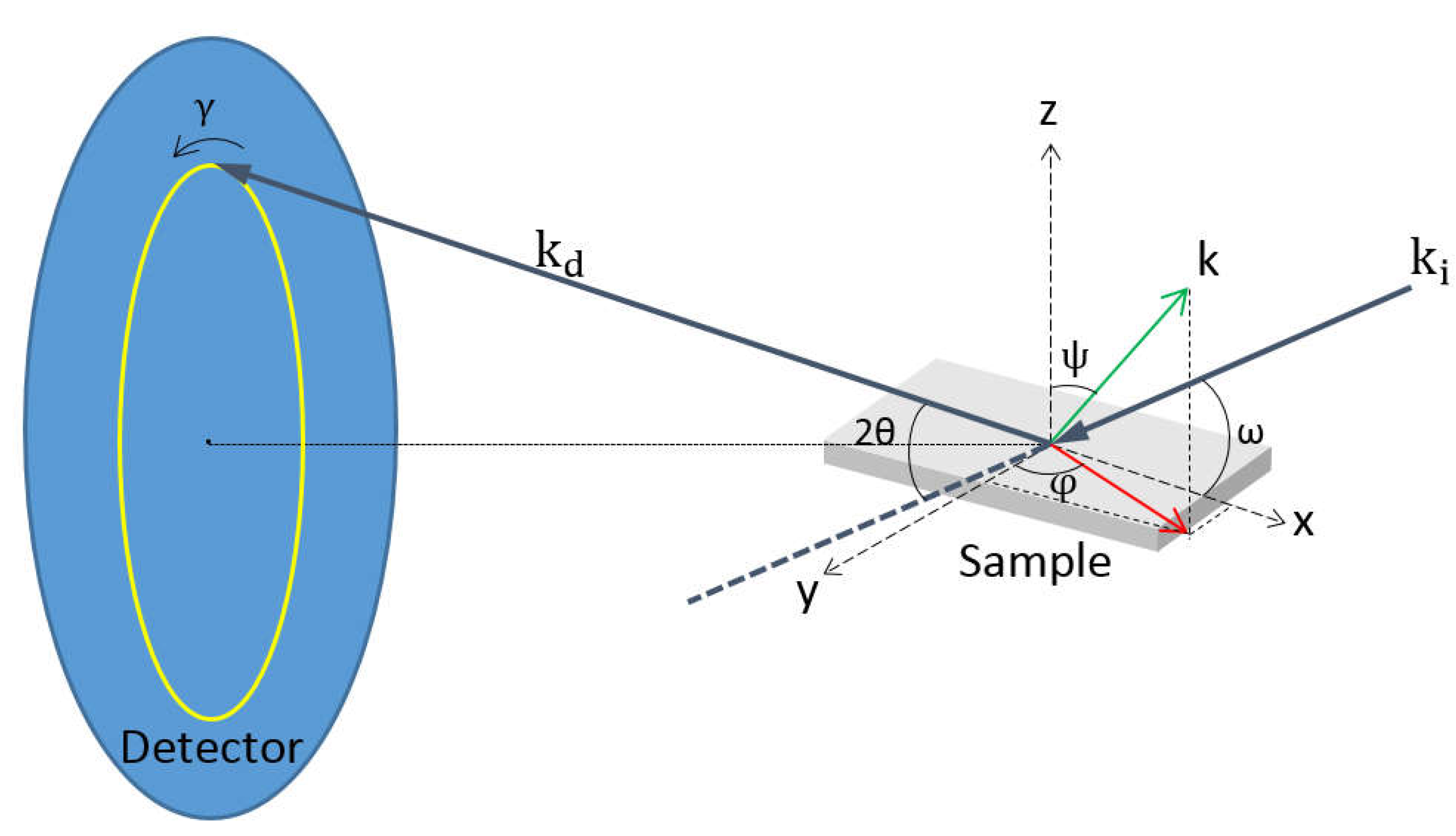
XRD is widely used to measure the elastic strain in crystalline material [8,9]. The experimental geometry of the system is presented in Figure 3. The method is used in reflexion. The samples of plane geometry are at a fixed distance of an area detector. The samples are cylinders of radius 6 mm and thickness 4 mm. The energy of 20 keV (optimum for photons flux on BM02) is well adapted to optimize the film response. A XRD diagram has been recorded using an area detector (FReLoN, ESRF, Grenoble, France), which is large enough to extract the stresses evolution in both the film and the metal, and fast enough to obtain data in real time, as in previous experiments [4].

The beamline is equipped with a goniometer, a sample carrier, an area detector, and two photodiodes. The first photodiode is placed in front of the sample and makes it possible to know the flux of incoming photons. The second photodiode is placed behind the sample and along the beam axis to allow alignment of the sample surface with the beam, which is important for height adjustment.

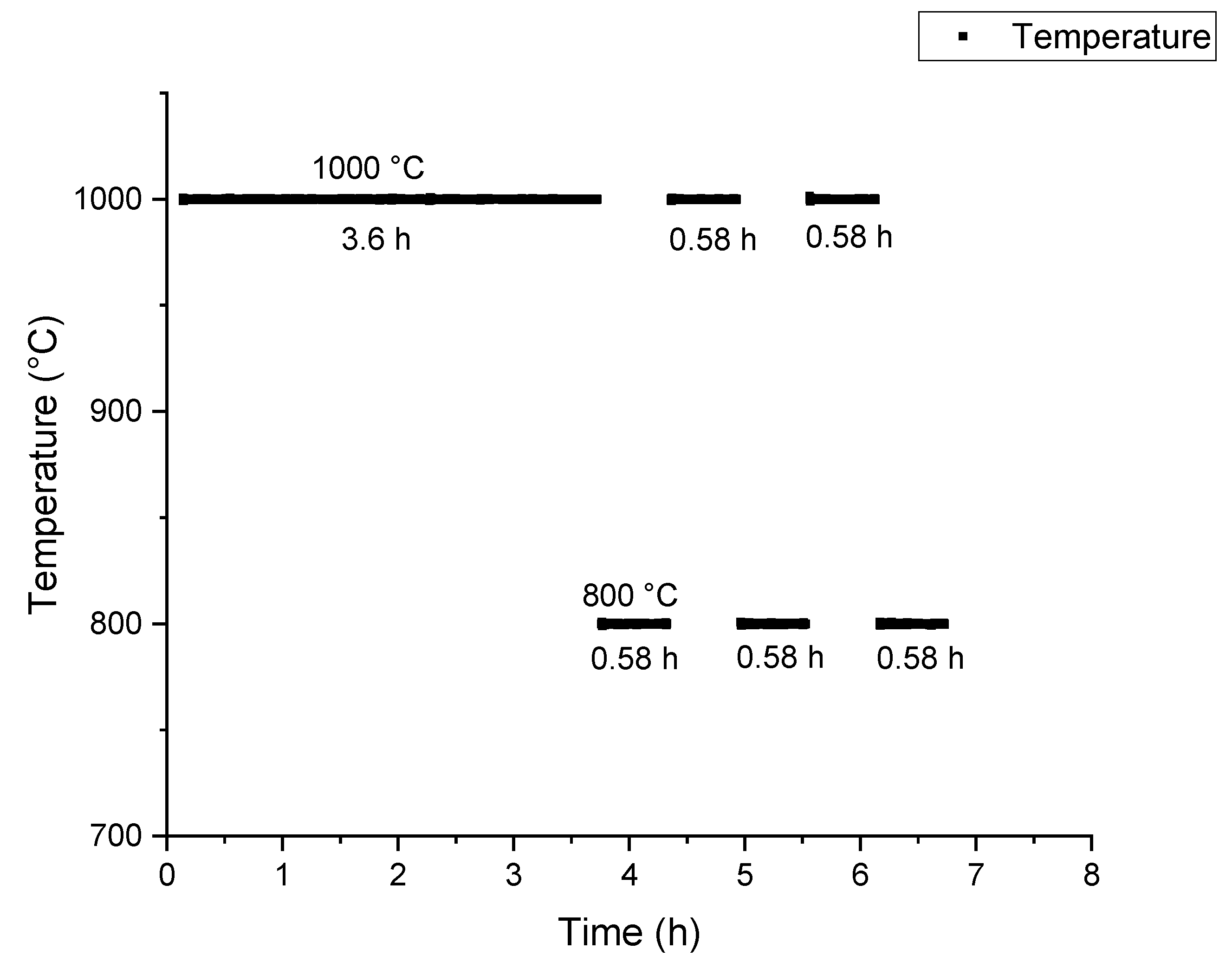
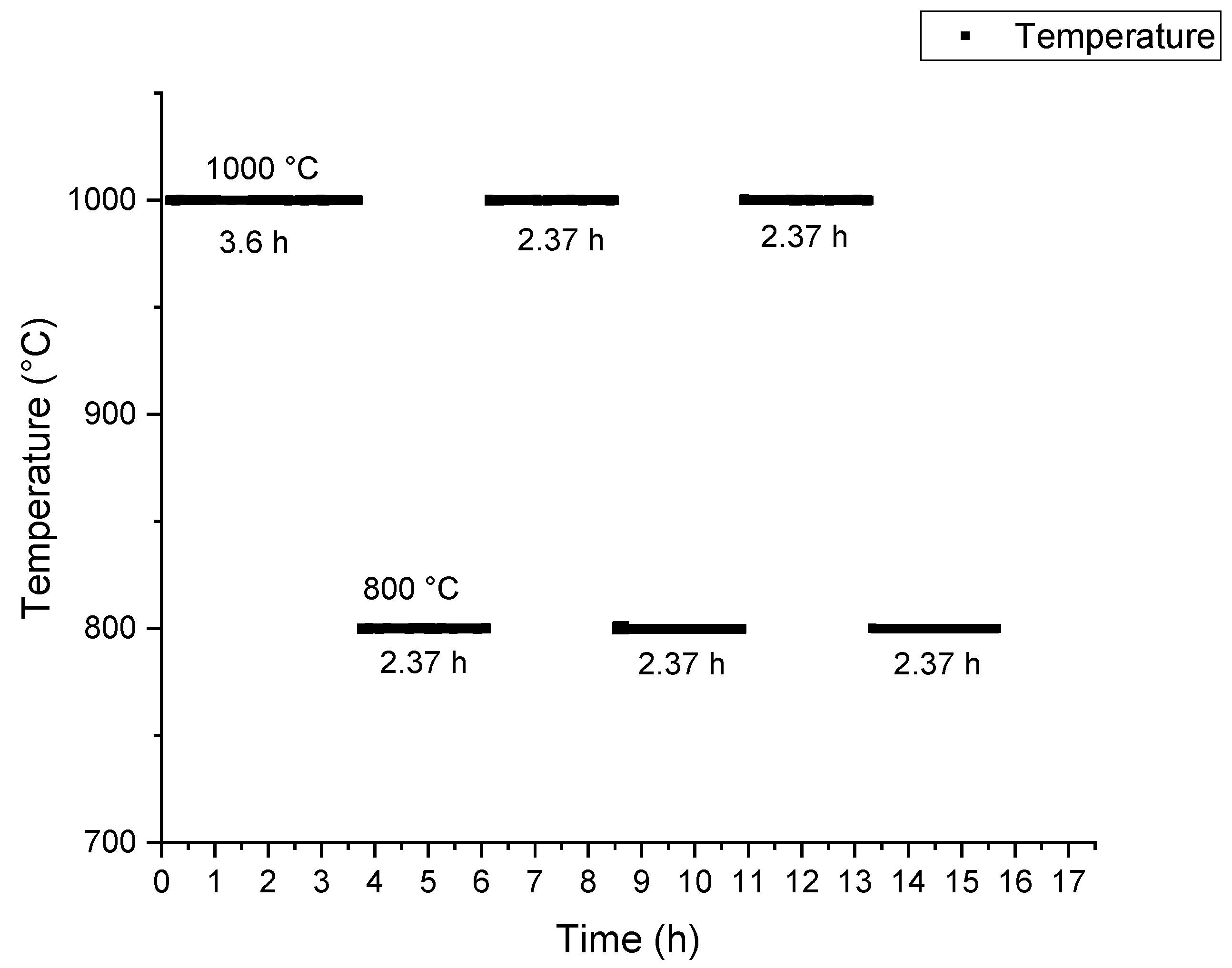
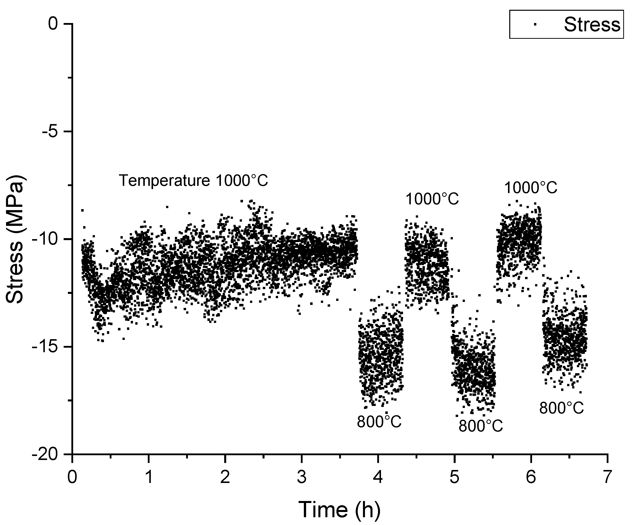
An induction furnace (ESRF, Grenoble, France) was used to simultaneously carry out oxidations with in-situ measurements and especially strain measurements during this oxidation. The induction furnace was provided by the Sample Environment Support Service of ESRF. The system was driven by a high-power generator (maximum 3kW). The sample carrier is a cylindrical support, surrounded by the induction coil with 7 mm diameter and 4 mm depth. A thermocouple is placed at the bottom of this support to control and regulate the temperature (the temperature can reach a maximum value of 1600 °C). The temperature on the surface of the sample was measured by a pyrometer (FAR, model FMPI, Riverview, Michigan, USA). The speed of heating and cooling can vary between 1 °C/min and 500 °C/min with a temperature of accuracy +/-1 °C. The main advantage of this furnace is its ability to heat or cool very quickly (thermal characteristic time of the furnace with our metallic specimen is around 13 s), with a good control of the heating and cooling speeds, which is an advantage to develop particular experiments (thermal cycling or temperature jumps. However, even if the use of a thermocouple and a pyrometer allows a correct knowledge of the oxidation temperature, it cannot be ignored that there may be a temperature gradient between the top and bottom faces of the sample (in contact with the bottom thermocouple). This may generate non-homogeneous expansion of the samples and may disturb especially disturb the height adjustment. The induction furnace is used for the oxidation of samples in air.

The X-ray beam size is 1 mm × 1 mm and the angle of incidence is 5°. The detector is located at a distance of 22 cm from the center of the goniometer. This detector makes an angle of 18° with the incident beam.

The calibration of the detector FReLoN was carried out using an ideal silicon powder as reference (NIST SRM640), in order to adjust the correspondence between pixel and angular degrees. The calibrant powders and samples have been placed at point O using the absorption profile of the sample from the direct beam recorded by a photodiode placed behind the sample position. The calibration is a very important step because a poor positioning of the camera can induce an offset at the pixels and, subsequently, an offset on the positions of the Debye-Scherrer rings.

In order to make the sample surface parallel to the beam, adjustment steps are required before each experiment to have a better accuracy. The procedure for adjustment of the flatness of the sample is as follows.

• Note the detected intensity of the uncut incident beam
• Adjust the sample to partially cut off the incident beam, detected intensity is then less than the previous intensity
• Rotate the sample around the axis to find the ideal position, for which the detected intensity is maximum. After this adjustment, the surface of the sample is then parallel to the incident beam
• Adjust precisely the height of the sample so that the detected intensity is equal to the ideal position

Because of all these complex steps and even with all calibration and adjustment processes, it is necessary, to obtain a correct stress value, to propose a correction method for possible errors or systematic bias such as beam deviation. It is explained in Section 2.3.

The associated stress can be determined thanks to the sin² $\mathsf{\psi }$ method, and using the radiocrystallographic elastic coefficients. Because the material consists of randomly oriented crystallites, Bragg’s law is applied to evaluate the changes of distance between crystallographic planes and taking into account the diffraction geometry (Figure 3). Then, rings are obtained with the help of an area detector. From [9], a relation is given to transform ψ as a function of θ and γ.

$$\cos \mathsf{\psi }=\sin \left(\mathsf{\theta }\right)\sin \left(\mathsf{\omega }\right)+\cos \left(\mathsf{\gamma }\right)\cos \left(\mathsf{\omega }\right)\cos \left(\mathsf{\theta }\right),$$

(1)

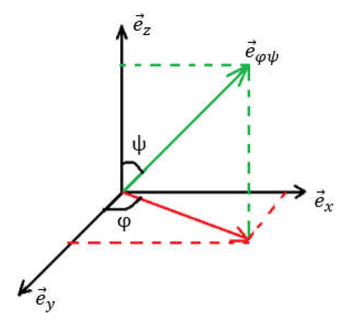
ψ is the angle between the normal to the surface and the normal to the diffracting planes, 2θ is the angle between the incident beam and the diffracted beam, ω is the incident angle, and γ is the angle between the vertical passing through the position of the direct beam and a given position on the diffraction ring.

Thus, each gamma value is related to ψ and the diffraction patterns are fitted for each ψ value, to obtain the corresponding d-spacing. Afterwards, the sin²ψ method is used to determine the associated stress. In the present study, the measured strain corresponds to the average through a depth of a few microns below the surface of the metallic sample.

2.2.2. Sin²ψ Method

When a material is deformed, the interreticular distance ${\mathrm{d}}_{\mathrm{hkl}}$ between crystallographic planes will extend or contract that causes a shift in the rings position in the diffraction pattern; the rings position correspond to the mean radius of the diffraction rings. In turn, the changes of distance between crystallographic planes can be evaluated by measurement of this angular shift, so that the elastic strain can be determined (Figure 4).

The coordinate system (x, y, z) is an orthonormal coordinate system that is linked to the sample. The direction ${\overrightarrow{\mathrm{e}}}_{\mathsf{\phi }\mathsf{\psi }}$ is the normal to the diffracting plans. The deformation on the direction ${\overrightarrow{\mathrm{e}}}_{\mathsf{\phi }\mathsf{\psi }}$ is:

$${\mathsf{\epsilon }}_{\mathsf{\psi }\mathsf{\phi }}={\overrightarrow{\mathrm{e}}}_{\mathsf{\phi }\mathsf{\psi }}·\stackrel{=}{\mathsf{\epsilon }}·{\overrightarrow{\mathrm{e}}}_{\mathsf{\phi }\mathsf{\psi }},$$

(2)

with

$${\overrightarrow{\mathrm{e}}}_{\mathsf{\phi }\mathsf{\psi }}=\sin \mathsf{\psi }\cos \mathsf{\phi }{\overrightarrow{\mathrm{e}}}_{\mathrm{x}}+{\sin \mathsf{\psi }\sin \mathsf{\phi }\overrightarrow{\mathrm{e}}}_{\mathrm{y}}+{\cos \mathsf{\psi }\overrightarrow{\mathrm{e}}}_{\mathrm{z}},$$

(3)

$\stackrel{=}{\mathsf{\epsilon }}$ is the symmetric strain tensor for small deformation:

$$\stackrel{=}{\mathsf{\epsilon }}=\left(\begin{array}{ccc}{\mathsf{\epsilon }}_{\mathrm{xx}}& {\mathsf{\epsilon }}_{\mathrm{xy}}& {\mathsf{\epsilon }}_{\mathrm{xz}}\\ {\mathsf{\epsilon }}_{\mathrm{xy}}& {\mathsf{\epsilon }}_{\mathrm{yy}}& {\mathsf{\epsilon }}_{\mathrm{yz}}\\ {\mathsf{\epsilon }}_{\mathrm{xz}}& {\mathsf{\epsilon }}_{\mathrm{yz}}& {\mathsf{\epsilon }}_{\mathrm{zz}}\end{array}\right),$$

(4)

The strain in the direction ${\overrightarrow{\mathrm{e}}}_{\mathsf{\phi }\mathsf{\psi }}$ is developed:

$${\mathsf{\epsilon }}_{\mathsf{\psi }\mathsf{\phi }}=\left({\mathsf{\epsilon }}_{\mathrm{xx}}{\cos }^2\mathsf{\phi }+{\mathsf{\epsilon }}_{\mathrm{yy}}{\sin }^2\mathsf{\phi }+{\mathsf{\epsilon }}_{\mathrm{xy}}\sin 2\mathsf{\phi }-{\mathsf{\epsilon }}_{\mathrm{zz}}\right){\sin }^2\mathsf{\psi }+\left({\mathsf{\epsilon }}_{\mathrm{xz}}\cos \mathsf{\phi }+{\mathsf{\epsilon }}_{\mathrm{yz}}\sin \mathsf{\phi }\right)\sin \left(2\mathsf{\psi }\right)+{\mathsf{\epsilon }}_{\mathrm{zz}},$$

(5)

The strain in the direction ${\overrightarrow{\mathrm{e}}}_{\mathsf{\phi }\mathsf{\psi }}$ can also be obtained by comparing the unstrained distance $d_0$ between crystallographic planes with the strained distance d.

$${\mathsf{\epsilon }}_{\mathsf{\psi }\mathsf{\phi }}=\ln \left(\frac{\mathrm{d}}{{\mathrm{d}}_0}\right)=\ln \left(\frac{{\sin \mathsf{\theta }}_0}{\sin \mathsf{\theta }}\right),$$

(6)

The sin²ψ relation in strain is obtained by combining the two equations (Equations (5) and (6)), which is a direct manifestation of the relationship between the angular shift and the strain.

$$\ln \left(\frac{{\sin \mathsf{\theta }}_0}{\sin \mathsf{\theta }}\right)=\left({\mathsf{\epsilon }}_{\mathrm{xx}}{\cos }^2\mathsf{\phi }+{\mathsf{\epsilon }}_{\mathrm{yy}}{\sin }^2\mathsf{\phi }+{\mathsf{\epsilon }}_{\mathrm{xy}}\sin 2\mathsf{\phi }-{\mathsf{\epsilon }}_{\mathrm{zz}}\right){\sin }^2\mathsf{\psi }+\left({\mathsf{\epsilon }}_{\mathrm{xz}}\cos \mathsf{\phi }+{\mathsf{\epsilon }}_{\mathrm{yz}}\sin \mathsf{\phi }\right)\sin \left(2\mathsf{\psi }\right)+{\mathsf{\epsilon }}_{\mathrm{zz}},$$

(7)

If we assume that elasticity of the material is linear, homogeneous and isotropic, i.e. without macroscopic texture, the conversion of elastic strain into stress can be done by using the Hooke’s model according to:

$$\stackrel{=}{\mathsf{\epsilon }}=\frac{1+\mathsf{\nu }}{\mathrm{E}}\stackrel{=}{\mathsf{\sigma }}-\frac{\mathsf{\nu }}{\mathrm{E}}\mathrm{trace}(\stackrel{=}{\mathsf{\sigma }})\stackrel{=}{\mathrm{I}},$$

(8)

with trace $\stackrel{=}{\mathsf{\sigma }}$ is the first invariant of the stress tensor and $\stackrel{=}{\mathrm{I}}$ is the three-dimensional (3D) identity tensor. With the assumption of transverse isotropy for an in-plane stress state, i.e., ${\mathsf{\sigma }}_{i\mathrm{z}}=0$ with i = x, y or z, we have the symmetric stress tensor:

$$\stackrel{=}{\mathsf{\sigma }}=\left(\begin{array}{ccc}{\mathsf{\sigma }}_{\mathrm{xx}}& {\mathsf{\sigma }}_{\mathrm{xy}}& 0\\ {\mathsf{\sigma }}_{\mathrm{xy}}& {\mathsf{\sigma }}_{\mathrm{yy}}& 0\\ 0& 0& 0\end{array}\right),$$

(9)

Moreover, we consider that there is no shear stress and we suppose the absence of a stress gradient.

$$\stackrel{=}{\mathsf{\sigma }}=\left(\begin{array}{ccc}\mathsf{\sigma }& 0& 0\\ 0& \mathsf{\sigma }& 0\\ 0& 0& 0\end{array}\right),$$

(10)

There is presently no experimental verification of the absence of stress gradient. However, previous works on the same material have proved with different techniques (XRD, Raman spectroscopy) with different gauge volumes that the stress is of the same magnitude for different depth in the material [4,5,6,10]. Because of the sin²ψ curve obtained, it is experimentally proved for almost all the oxidation time that the system presents transverse isotropy. Moreover, by changing φ, we have also verified that such systems can be assumed as equi-biaxial.

The sin²ψ relation in stress is acquired by simplification of the equation, which emphasizes the connection between the angular shift and the stress.

$$\mathrm{Ln}\left(\frac{{\sin \mathsf{\theta }}_0}{\sin \mathsf{\theta }}\right)=\frac{1+\mathsf{\nu }}{\mathrm{E}}{\mathsf{\sigma }\sin }^2\mathsf{\psi }-\frac{\mathsf{\nu }}{\mathrm{E}}2\mathsf{\sigma },$$

(11)

By using the radiocrystallographic elastic coefficients S₁ and ½ S₂, the sin²ψ relation becomes:

$$\ln \left(\frac{1}{\sin \mathsf{\theta }}\right)=\frac{1}{2}{\mathrm{S}}_{2\left(\mathrm{hkl}\right)}{\mathsf{\sigma }\sin }^2\mathsf{\psi }+2{\mathrm{S}}_{1\left(\mathrm{hkl}\right)}\mathsf{\sigma }-\ln \left({\sin \mathsf{\theta }}_0\right),$$

(12)

The slope of this line corresponds to $\frac{1}{2}{\mathrm{S}}_{2\left(\mathrm{hkl}\right)}\mathsf{\sigma }$ and the intercept corresponds to $2{\mathrm{S}}_{1\left(\mathrm{hkl}\right)}\mathsf{\sigma }-\ln \left({\sin \mathsf{\theta }}_0\right)$. Since we already have the radiocrystallographic elastic coefficients (

Table 2. Radiocrystallographic elastic coefficients.

	800 °C
Stiffness	Cr2O3 (104)	Cr2O3 (110)	Cr2O3 (116)	Ni30Cr (111)
${\mathrm{S}}_1$ (TPa−1)	−0.824	−1.018	−0.805	−1.622
0.5 $\times {\mathrm{S}}_2$ (TPa−1)	3.987	4.557	3.927	6.886
	1000 °C
Stiffness	Cr2O3 (104)	Cr2O3 (110)	Cr2O3 (116)	Ni30Cr (111)
${\mathrm{S}}_1$ (TPa−1)	−0.817	−1.010	−0.867	−1.837
0.5 $\times {\mathrm{S}}_2$ (TPa−1)	3.999	4.561	4.136	7.752

) for different families of (hkl) planes, we can calculate the stress in the oxide and in the metal.

Table 2 gives the radiocrystallographic elastic coefficients for different families of (hkl) planes at 800 and 1000 °C [11,12].

2.2.3. Data Processing

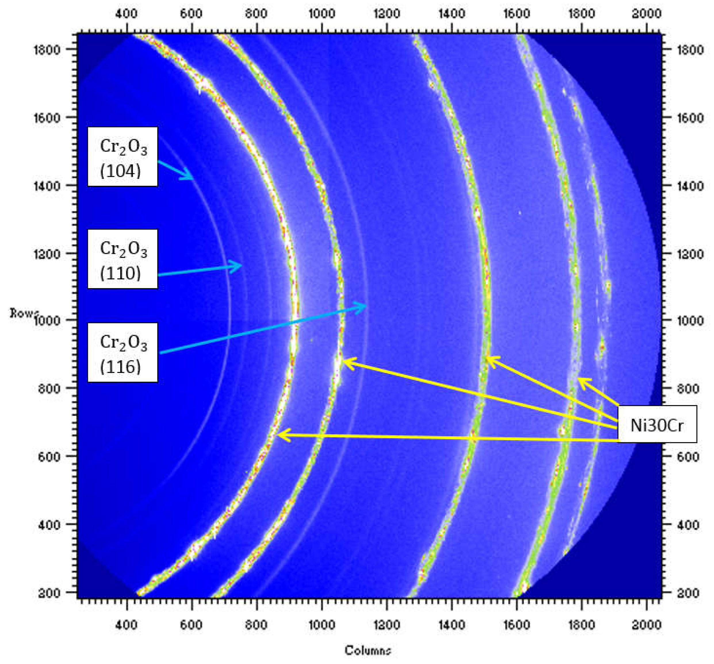
Raw data (see example in Figure 5) are images of the diffracted rings. It has to be analyzed to get the stress in the oxide layers and in the metal. For a stress-free material, the data must draw perfect arcs of circles. Figure 5 shows an example recorded for the NiCr/Cr₂O₃-system. As we can see in Figure 5, the intensity for the metal rings are not as homogenous as for the oxide rings. This is mainly due to a grain size effect, which is bigger in the metal (around 400 µm [13]) than in the oxide (less than 1 µm [14]) when compared to the beam size. With time, oxide rings become more continuous. Except for the very beginning of the oxidation, we are easily able to fit the peaks because of the good resolution of the area detector and it is sufficient for sin²ψ method.

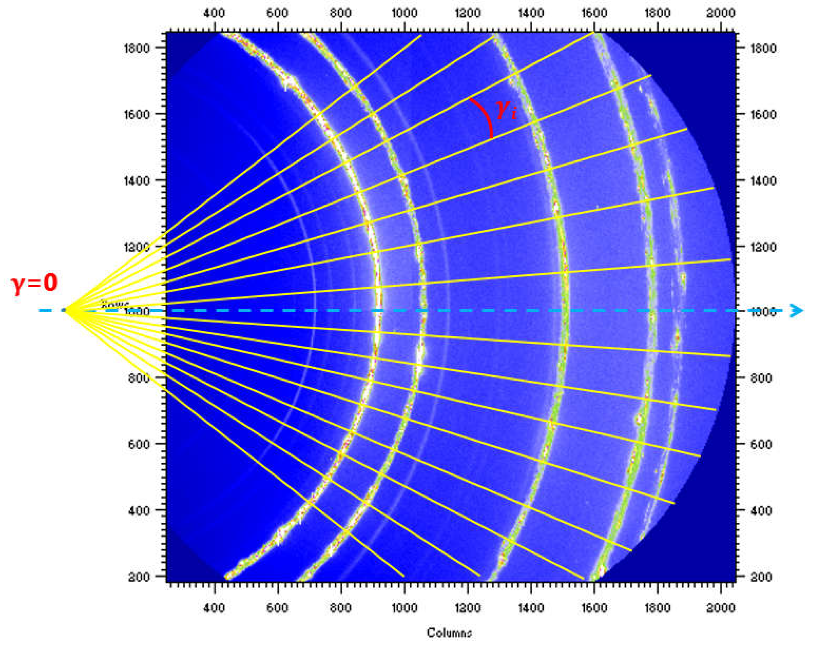
To perform the analysis, the rings were subdivided into 128 sectors γ whose values are between {−61.5 ° and +65.5 °} with a step of 1° (Figure 6).

From these data, it is possible to plot the intensities of each sector γ as a function of 2θ, giving a diffraction diagram. The peaks studied for the chromium oxide are (104), (110), (116), and the peak for the nickel-chromium alloy is (111). The 2θ free of stress reference positions are summarized in

Table 3. Reference positions for the free of stress diffraction peaks that are used in [15].

Plane (hkl) Cr2O3	(104)	(110)	(116)	Plane (hkl)	NiCr (111)
2θ Theoretical (°)	13.25	14.30	21.20	2θ Theoretical (°)	17.22

.

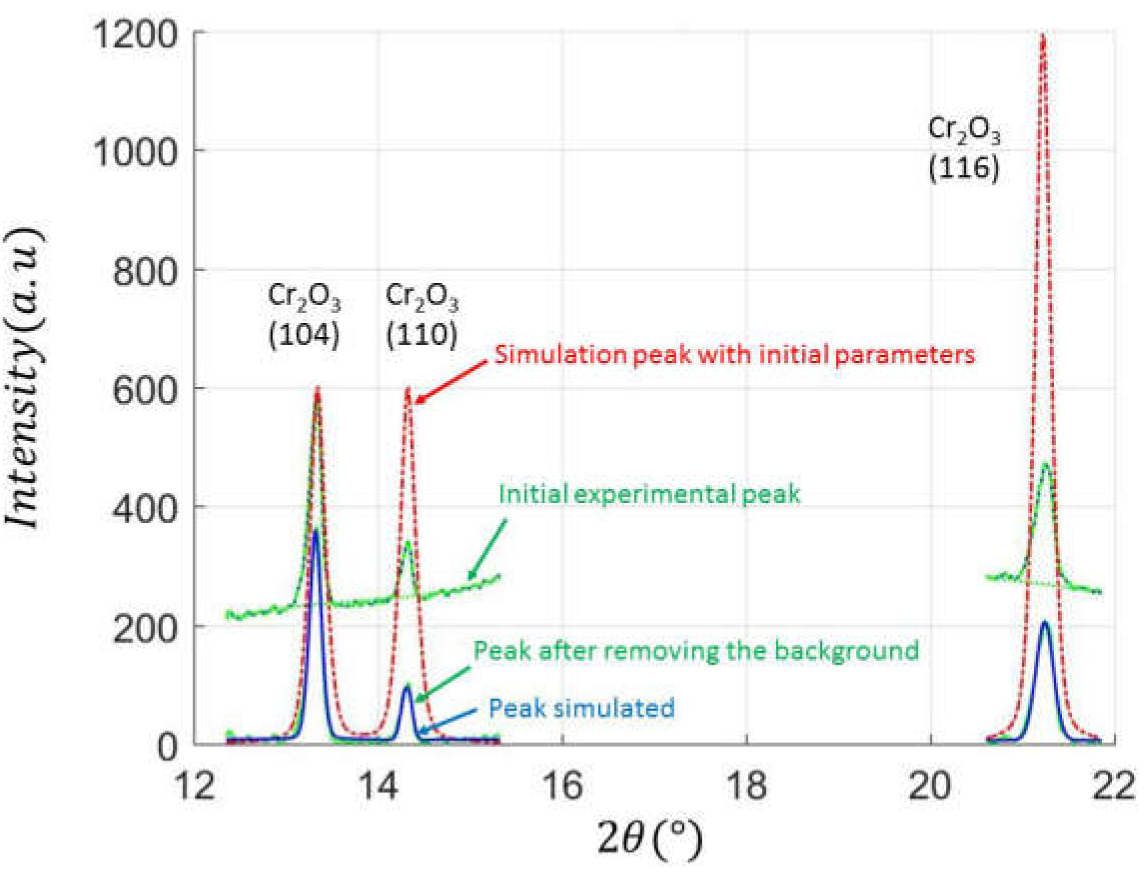
Each diffraction diagram has to be simulated by using different functions and after background subtraction. Indeed, it is necessary to minimize the influence of the background. Four main distribution functions have been tested to simulate the peaks profile, which are Gauss, Lorentz, Pearson 7, and Pseudo-Voigt. Concerning the background, we choose a polynomial relationship. In addition, the order of the polynomial relationship is also tested. In the computing procedure, we can simulate the peak distribution and the background noise together or separately.

Figure 7 shows an example, which simulates the peak shape and the background separately. It shows four curves, which are initial experimental peak, simulated peak with initial parameters, experimental peak after removing the background, and simulated peak with final parameters. Initial experimental peak corresponds to the initial experimental data. Simulated peak with initial parameters is obtained with the initial set of parameters used in the distribution function. The position, width and intensity of peaks are close to the simulation peak with these initial parameters. Then by applying an optimization method (non-linear fitting function in Matlab software), we can simulate the peak more correctly and find the final parameters (position, width, and intensity). Moreover, thresholds enable obtaining a good quality for fitting process. For example, we have a threshold for intensity: an intensity value below this threshold leads to consider the fitting of the peak as not good, etc. To obtain the peak after removing the background, we simulate the background by using a polynomial relationship and remove the simulated results from the initial experimental data. Finally, the peak is simulated with one of the distribution functions mentioned before, by using the final parameters.

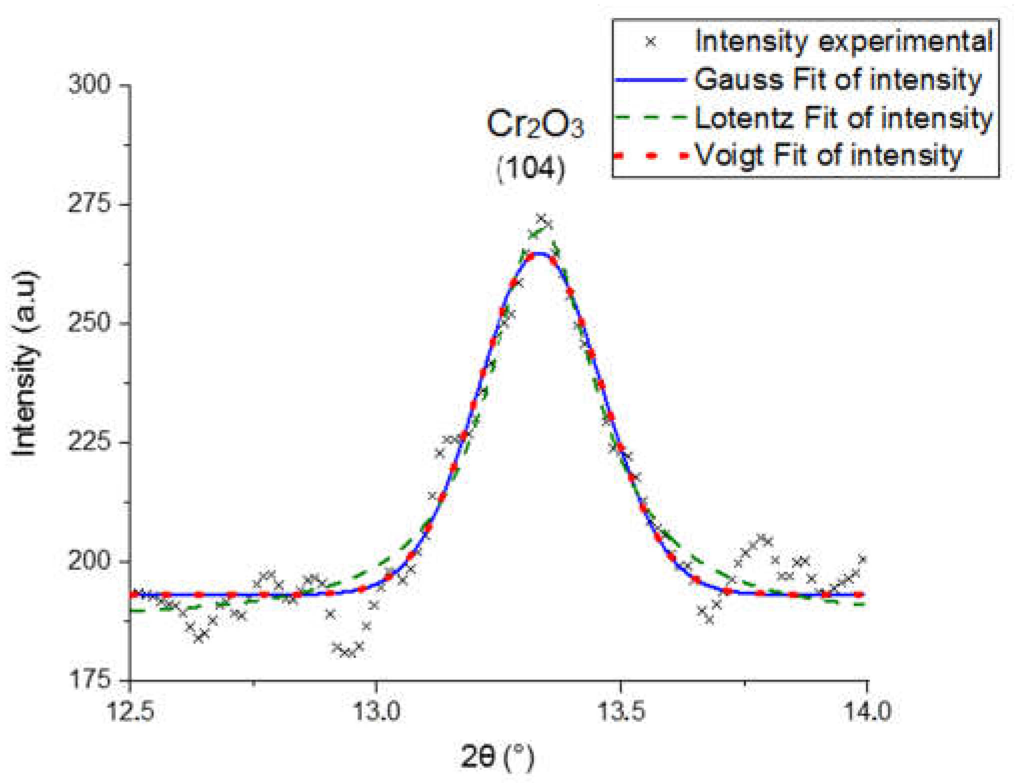
Figure 8 shows the results that were obtained for the different distribution functions. The simulation results are quite similar for the different output parameters obtained, such as intensity, position, and width of the peak. Finally, to choose the best function, we need to test systematically this procedure by considering a significant number of experimental data.

After comparing different quality indicators (such as slope, average value, average absolute difference and difference between maximum and minimum), we consider that a Pearson 7 distribution function with a simultaneous background simulated by an order 3 polynomial function lead to a maximization of the fitting quality. Therefore, these parameters have been considered for the simulation of all the data.

To summarize, the first two peaks are fitted together and the third peak is fitted by itself. Peaks are simulated first to hang the optimization of parameters with some criteria/error to stop the optimization. Then a simulation in return is performed with the optimized parameters to check visually the calculation. For the background noise, it is typically a cubic power law used for the fitting. Even with the procedure of calibration of the detector, it is not possible to remove all of the background noise. All of this procedure has been automated in a Matlab software. Moreover, we randomly selected 100 pictures to apply this procedure for different simulation models, which correspond to a relatively stable period.

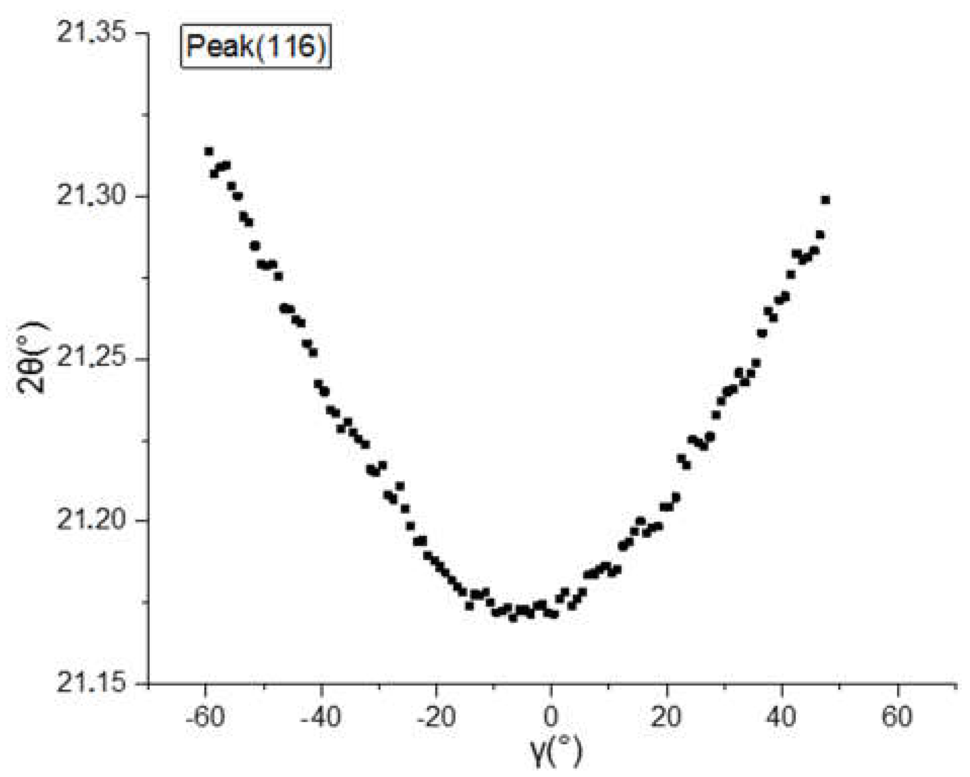
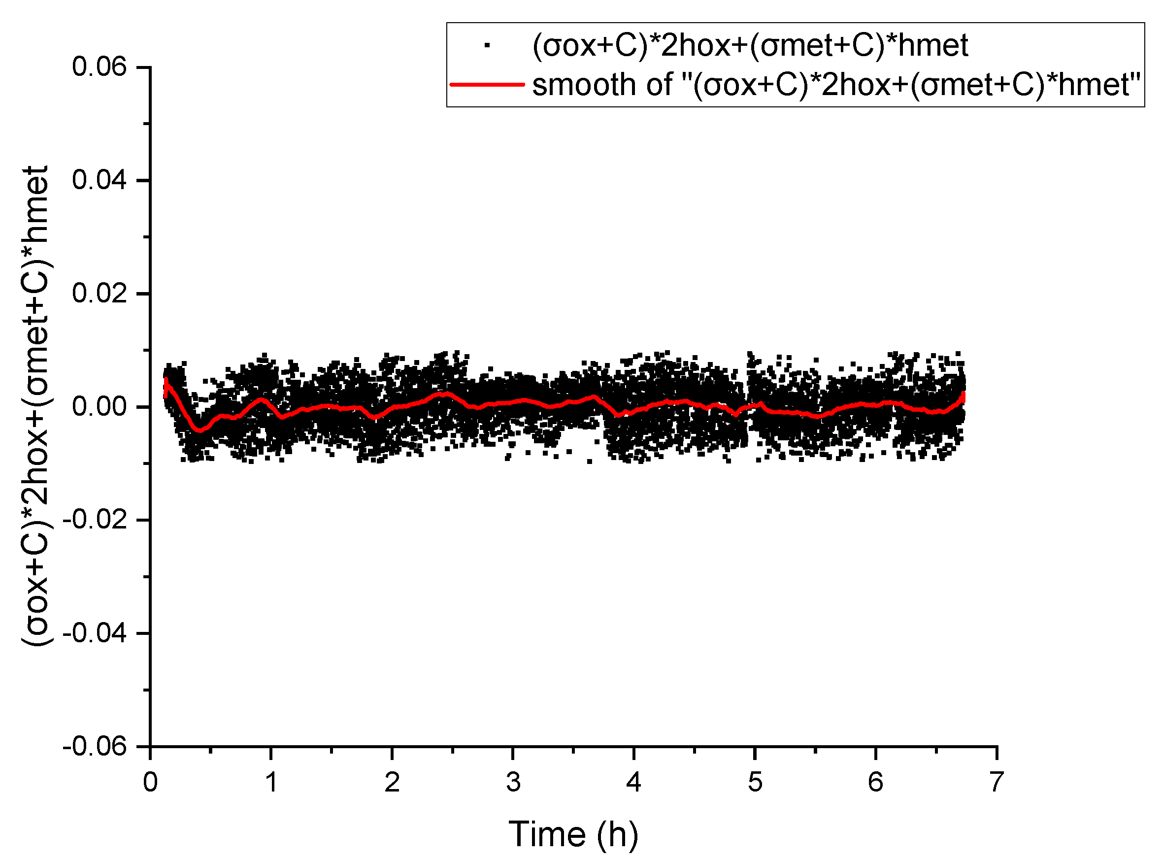
Afterwards, to visualize the stress influence, the 2θ position can be plotted as a function of γ for a given peak (Figure 9).

Figure 9 shows an example of 2θ versus γ for the peak (116) in the oxide. A symmetrical variation of the positions 2θ is observed, which corresponds to a stressed material. The same trend (not shown) is observed in the metal.

To draw the curves of sin²ψ, different other quality criteria have also been defined in the computing process. For example, a criterion corresponds to the confidence interval around the linear fit that control the removal of abnormal points. In addition, the correlation coefficient of the fit and the difference between the first point and the last point of the linear fit are also used to assess the quality of the fit. If all of these criteria are satisfied, we can consider that the fitted curves are correct.

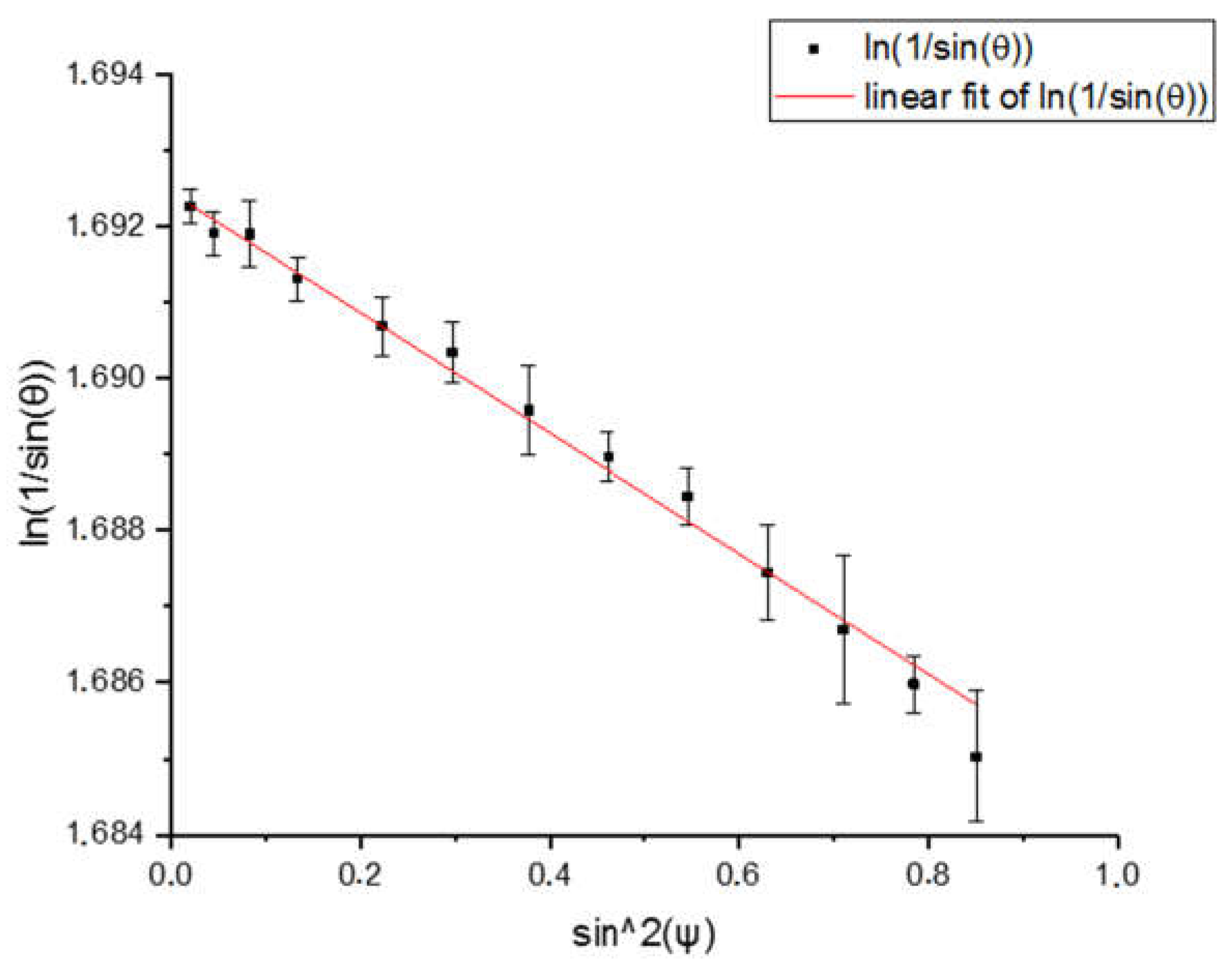
Figure 10 gives an example of result obtained for ψ < 0. The trend for ψ > 0 is quite similar (but is not shown in this article).

In order to more legibly display the results, we calculate an average for every five data, which are indicated by the black points in Figure 10. The “error” bar corresponds here to the range for which we can find the other points. It is calculated from the difference value between every five data. The slope of this line corresponds to $\frac{1}{2}{\mathrm{S}}_{2\left(\mathrm{hkl}\right)}\mathsf{\sigma }$ and the intercept to $2{\mathrm{S}}_{1\left(\mathrm{hkl}\right)}\mathsf{\sigma }-\ln \left({\sin \mathsf{\theta }}_0\right)$. The range of variation of the values $\ln \left(\frac{1}{\sin \mathsf{\theta }}\right)$ is 7.2 × 10⁻³. The error bar is in the range 2.3 × 10⁻⁴ to 9.8 × 10⁻⁴, which is small when compared to the variation of the values for$\ln \left(\frac{1}{\sin \mathsf{\theta }}\right)$. The relationship between $\ln \left(\frac{1}{\sin \mathsf{\theta }}\right)$ and ${\sin }^2\mathsf{\psi }$ is well linear, which corresponds to equation (12). The stress value corresponds to only one point in the stress-time curves evolution. After repeating this procedure for all the experimental pictures/times, we can finally get the stress-time curve for the different (hkl) oxide families.

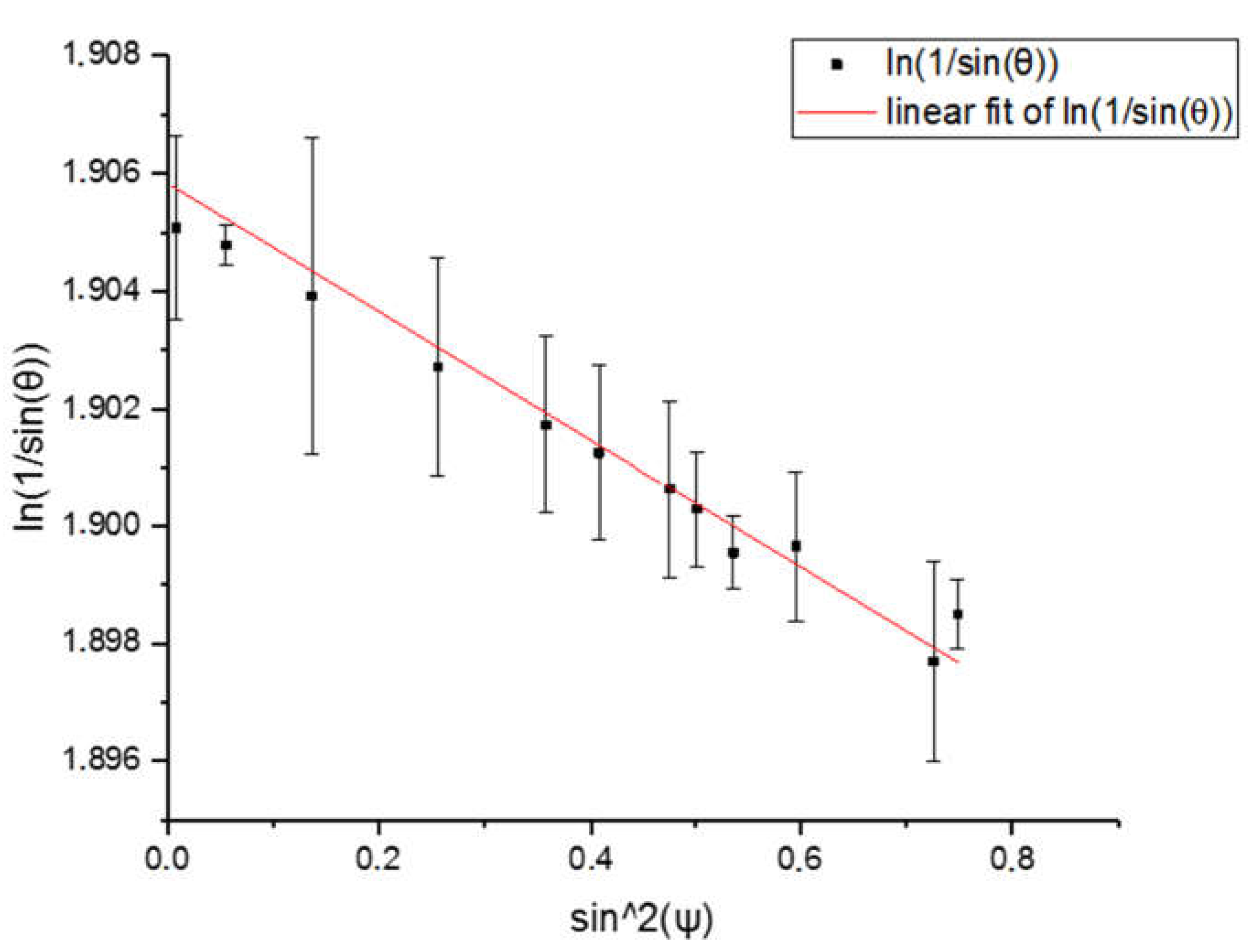
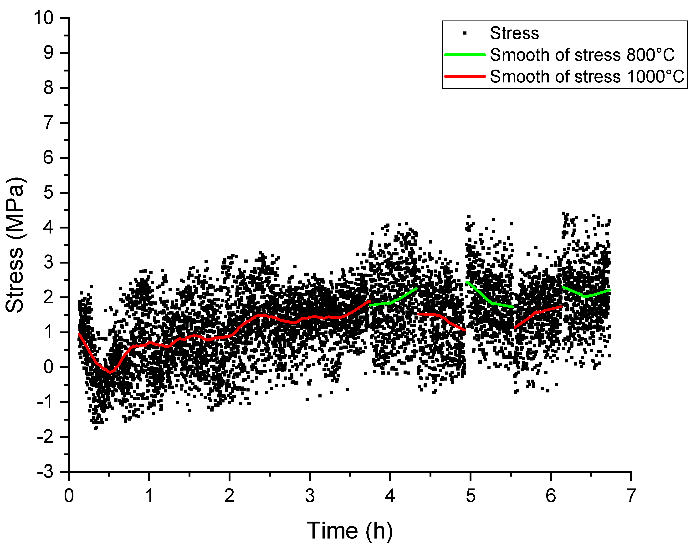
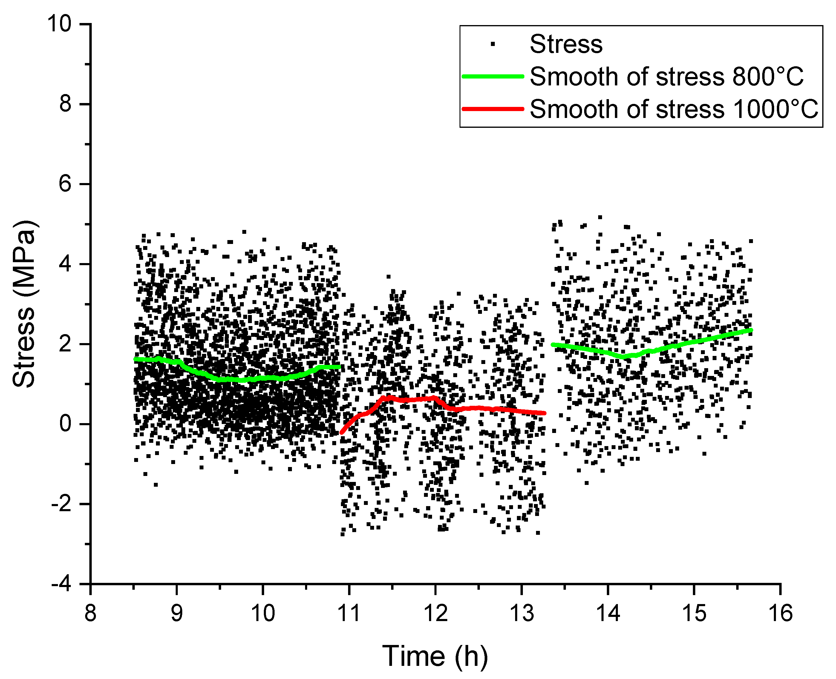
The same analysis has been undertaken for the metal. For a better comparison of the results between oxide and metal, the same kind of display has been adopted. Figure 11 shows an example of the results obtained. The error bar is from 3.5 × 10⁻⁴ to 2.7 × 10⁻³, which is higher than the error bar in the oxide. However, we can again consider with confidence that the relationship between $\ln \left(\frac{1}{\sin \mathsf{\theta }}\right)$ and ${\sin }^2\mathsf{\psi }$ is linear, as in the oxide layer. Therefore, after repeating this procedure for all of the experimental data, the stress-time curve for the (111) metal peak can be also obtained.

Table 4. Comparison of the data quality obtained from the fitting procedure.

Phase	Variation of $\mathbf{ln}\mathbf{\left(}\frac{\mathbf{1}}{\mathbf{s}\mathbf{i}\mathbf{n}\mathsf{\theta }}\mathbf{\right)}$	Minimum Error Bar	Maximum Error Bar	Average Error Bar	Proportion of Average Error Bar
Oxide	7.2 × 10−3	2.3 × 10−4	9.8 × 10−4	4.8 × 10−4	6.7%
Metal	7.4 × 10−3	3.5 × 10−4	2.7 × 10−3	1.3 × 10−3	17.6%

shows the data quality comparison for oxide and metal.

As written before, the error bar is calculated from the difference between five data. By comparing the values of this error bar, we can check the data quality of the results in oxide and metal. The proportion of average error bar is the proportion of average error bar in the variation of $\ln \left(\frac{1}{\sin \mathsf{\theta }}\right)$. The variation range of $\ln \left(\frac{1}{\sin \mathsf{\theta }}\right)$ is very similar in oxide and in metal. The maximum error bar and the average error bar are larger in metal than in oxide. The proportion of average error bar is also larger in metal than in oxide. That is to say, from these criteria, the data quality of the results in oxide is a little bit better than in metal.

2.2.4. Stress versus Time Results

By using the method described above, the stress-time curves in metal and oxide are obtained. Because of the thermal cyclic loading, the stress in both oxide and metal changes with temperature. Figure 12 and Figure 13 show the results that were obtained for R0.58.

Figure 12 and Figure 13 evidence that the stress in substrate and oxide is compressive. When the temperature changes, the jump between two plateaus is clearly visible for both metal and oxide. It also indicates that the order of stress magnitude in the substrate is less than 10MPa, while it is in the range 1500–2000 MPa in the oxide.

In metal (Figure 12), we have calculated the average stress of all the plateaus under 1000 °C, which is −11 MPa. The difference between the maximum stress and the average stress is −2 MPa; the minimum stress and the average stress difference is 2.6 MPa. Therefore, the stress in metal is around −11 ± 3 MPa at 1000 °C. We have performed the same calculation for the other plateau at 800 °C, which shows that the stress is −15 ± 3MPa. Such calculations also indicate that the stress in oxide is around −1605 ± 100 MPa at 1000 °C and −2156 ± 100 MPa at 800 °C.

When considering previous works in literature [1,2,3] concerning the stress determination in such metal-oxide systems [5], the stress is usually compressive in oxide. Thus, assuming that stress is homogenous in both oxide and metal, the mechanical balance equation requires that the stress in substrate should be tensile. Therefore, in order to hold the mechanical balance equation, it is necessary to take into account the systematic errors occurring during the measurement. To this end, an offset has to be considered in the stress magnitude determination.

2.3. Stress Corrections

Different causes may explain the systematic errors and bias during the measurement. It includes, without exhaustivity:

• Dilatation correction: at the beginning of each temperature plateau, a procedure is applied to adjust the position of the sample; its height is corrected from the dilation effect. Therefore, the X-ray should irradiate the same place, whatever the temperature is. However, an uncertainty is associated to this correction step.
• Calibration procedure: to get the angular positions of the diffracted rings, it is necessary to establish a correspondence between the rings and pixels positions on the area images. To achieve such a goal, the obtained raw data have been systematically corrected by using references standard positions (NIST Silicon or Cr₂O₃) analyzed in the same diffraction conditions. However, an uncertainty is also associated to this procedure.

The mechanical balance equation overall metal and oxide can be expressed as:

$$\begin{array}{c}{{\displaystyle \int }}_0^{{\mathrm{h}}_{\mathrm{met}}}{\mathsf{\sigma }}_{\mathrm{met}}\left(\mathrm{z}\right)\times \mathrm{d}\mathrm{z}=-{\mathsf{\sigma }}_{\mathrm{ox}}\times 2\times {\mathrm{h}}_{\mathrm{ox}} , \end{array}$$

(13)

where ${\mathsf{\sigma }}_{\mathrm{ox}}$ is the stress in the oxide, ${\mathrm{h}}_{\mathrm{ox}}$ is the oxide thickness that depends on time t, ${\mathsf{\sigma }}_{\mathrm{met}}$ is the stress in the substrate, and ${\mathrm{h}}_{\mathrm{met}}$ is the thickness of the substrate. The influence of the oxide on the top and bottom surfaces is the main effect, which causes the apparition of residual stresses parallel to the oxide-metal interface in the metal. A symmetric oxidation is taken into account, thanks to the coefficient 2 in the mechanical balance equation in Equation (13).

We considered that the stress in metal may be divided into two parts. One part is the stress detected by XRD and that can be obtained with the ${\sin }^2\mathsf{\psi }$ method. The other part is the remaining part.

$$\begin{array}{c}{\mathsf{\sigma }}_{\mathrm{met}}\left(\mathrm{detected}\right)\times \mathrm{h}\left(\mathrm{detected}\right)+{\mathsf{\sigma }}_{\mathrm{met}}\left(\mathrm{rem}\right)\times \mathrm{h}\left(\mathrm{rem}\right)=-{\mathsf{\sigma }}_{\mathrm{ox}}\times 2\times {\mathrm{h}}_{\mathrm{ox}} , \end{array}$$

(14)

where ${\mathsf{\sigma }}_{\mathrm{met}}\left(\mathrm{detected}\right)$ is the stress in the detected part, $\mathrm{h}\left(\mathrm{detected}\right)$ is the corresponding detected thickness,${\mathsf{\sigma }}_{\mathrm{met}}\left(\mathrm{rem}\right)$ is the stress in the remaining part, and $\mathrm{h}\left(\mathrm{rem}\right)$ is the remaining thickness.

According to bibliography [1,2,3,5], it is assumed that the detected stress is larger than the remaining stress in the metal layer.

$$\begin{array}{c}{\mathsf{\sigma }}_{\mathrm{met}}\left(\mathrm{rem}\right)=\mathsf{\beta }\times {\mathsf{\sigma }}_{\mathrm{met}}\left(\mathrm{detected}\right), \mathsf{\beta }\le 1 , \end{array}$$

(15)

We have then:

$$\begin{array}{c}{\mathsf{\sigma }}_{\mathrm{met}}\left(\mathrm{detected}\right)\times \mathrm{h}\left(\mathrm{detected}\right)+\mathsf{\beta }\times {\mathsf{\sigma }}_{\mathrm{met}}\left(\mathrm{detected}\right)\times \mathrm{h}\left(\mathrm{rem}\right)=-{\mathsf{\sigma }}_{\mathrm{ox}}\times 2\times {\mathrm{h}}_{\mathrm{ox}} , \end{array}$$

(16)

$$\begin{array}{c}{\mathsf{\sigma }}_{\mathrm{met}}\left(\mathrm{detected}\right)=-\frac{{\mathsf{\sigma }}_{\mathrm{ox}}\times 2\times {\mathrm{h}}_{\mathrm{ox}}}{\mathrm{h}\left(\mathrm{detected}\right)+\mathsf{\beta }\times \mathrm{h}\left(\mathrm{rem}\right)} , \end{array}$$

(17)

with:

$$\begin{array}{c}\mathrm{h}\left(\mathrm{detected}\right)+\mathsf{\beta }\times \mathrm{h}\left(\mathrm{rem}\right)\le {\mathrm{h}}_{\mathrm{met}} , \end{array}$$

(18)

It implies that:

$$\begin{array}{c}\left|{\mathsf{\sigma }}_{\mathrm{met}}\left(\mathrm{detected}\right)\right|=\left|\frac{{\mathsf{\sigma }}_{\mathrm{ox}}\times 2\times {\mathrm{h}}_{\mathrm{ox}}}{\mathrm{h}\left(\mathrm{detected}\right)+\mathsf{\beta }\times \mathrm{h}\left(\mathrm{rest}\right)}\right|\ge \left|\frac{{\mathsf{\sigma }}_{\mathrm{ox}}\times 2\times {\mathrm{h}}_{\mathrm{ox}}}{{\mathrm{h}}_{\mathrm{met}}}\right|, \end{array}$$

(19)

By giving a homogeneous stress distribution in metal and oxide, we consider at first approximation the measured stress as equal to the global averaged stress in all of the metal part. That is to say, the absolute value of the detected stress under this hypothesis is a maximum value of the stress in metal. When considering this assumption, the mechanical balance equation overall metal and oxide can be expressed as:

$$\begin{array}{c}{\mathsf{\sigma }}_{\mathrm{ox}}\times 2\times {\mathrm{h}}_{\mathrm{ox}}+{\mathsf{\sigma }}_{\mathrm{met}}\times {\mathrm{h}}_{\mathrm{met}}=0,\end{array}$$

(20)

The oxide thickness ${\mathrm{h}}_{\mathrm{ox}}$ follows a parabolic evolution with oxidation time t that has already been evidenced for the present material with experimental characterization by Thermal Gravimetric Analysis [5]. We have:

$$\begin{array}{c}{\mathrm{h}}_{\mathrm{ox}}\left(\mathrm{t}\right)={\mathrm{k}}_{\mathrm{cp}}\sqrt{\mathrm{t}}, \end{array}$$

(21)

with ${\mathrm{k}}_{\mathrm{cp}}$ the parabolic kinetics parameter that relates to the parabolic rate mass parameter ${\mathrm{k}}_{\mathrm{mp}}$ obtained from experiments, as we have reported in

Table 5. The parabolic rate mass parameters that are used in [17].

Temperature (°C)	800	900	1000
${\mathrm{k}}_{\mathrm{mp}}$ ( ${\mathrm{g}}^2 {\mathrm{cm}}^{-4} {\mathrm{s}}^{-1}$)	2.18 × 10−13	6.08 × 10−13	5.56 × 10−12

.

$$\begin{array}{c} {\mathrm{k}}_{\mathrm{cp}}={\left(\frac{3\times \mathrm{M}\left({\mathrm{Cr}}_2{\mathrm{O}}_3\right)}{4\times \mathsf{\rho }\left({\mathrm{Cr}}_2{\mathrm{O}}_3\right)\times \mathrm{M}\left({\mathrm{O}}_2\right)}\right)}^2{\mathrm{k}}_{\mathrm{mp}},\end{array}$$

(22)

$\mathsf{\rho }\left({\mathrm{Cr}}_2{\mathrm{O}}_3\right)$ is the density of ${\mathrm{Cr}}_2{\mathrm{O}}_3$, $\mathrm{M}\left({\mathrm{Cr}}_2{\mathrm{O}}_3\right)$ is the molar mass of ${\mathrm{Cr}}_2{\mathrm{O}}_3$, $\mathrm{M}\left({\mathrm{O}}_2\right)$ is the molar mass of ${\mathrm{O}}_2$.

During oxidation, the change of metal thickness is very small. Therefore, we consider that ${\mathrm{h}}_{\mathrm{met}}$ is constant and equal to 4 mm.

In order to determine the offset and analyze the shift of stress in oxide and substrate, we propose two methods.

2.3.1. Correction with Method 1

Hypothesis 1. 

The offset is constant with time in each plateau, but it is different in oxide and in metal.

$$\begin{array}{c}({\mathsf{\sigma }}_{\mathrm{ox}}+{\mathrm{C}}_{\mathrm{ox}})\times 2\times {\mathrm{h}}_{\mathrm{ox}}+({\mathsf{\sigma }}_{\mathrm{met}}+{\mathrm{C}}_{\mathrm{met}})\times {\mathrm{h}}_{\mathrm{met}}=0,\end{array}$$

(23)

$$\begin{array}{c}\Rightarrow {\mathsf{\sigma }}_{\mathrm{ox}}\times \frac{2\times {\mathrm{h}}_{\mathrm{ox}}}{{\mathrm{h}}_{\mathrm{met}}}+{\mathsf{\sigma }}_{\mathrm{met}}=-{\mathrm{C}}_{\mathrm{ox}}\times \frac{2\times {\mathrm{h}}_{\mathrm{ox}}}{{\mathrm{h}}_{\mathrm{met}}}-{\mathrm{C}}_{\mathrm{met}}, \end{array}$$

(24)

By figuring the relationship ${\mathsf{\sigma }}_{\mathrm{ox}}\times \frac{2\times {\mathrm{h}}_{\mathrm{ox}}}{{\mathrm{h}}_{\mathrm{met}}}+{\mathsf{\sigma }}_{\mathrm{met}}$ in terms of $\frac{2\times {\mathrm{h}}_{\mathrm{ox}}}{{\mathrm{h}}_{\mathrm{met}}}$ (Figure 14), the slope of this line corresponds to $-{\mathrm{C}}_{\mathrm{ox}}$, which is the offset of the stress in oxide, whereas the intercept corresponds to $-{\mathrm{C}}_{\mathrm{met}}$ which is the offset of the stress in metal.

For each temperature plateau, we have simulated the data by a linear relationship. For example, Figure 14 shows the results of the linear fitting for plateaus 1 and 3. On one hand, the obtained equations for each plateau lead to the oxide offsets values of −965.8, −56,383, 12,015, 78,753, −15,170 and 1574 MPa. Some are much larger than the order of magnitude of the oxide stress itself. On the other hand, the obtained offset values for the metal are, respectively, 12.8, 70.3, 3.6, −62.1, 27.6, and −0.4 MPa. These values compare quite well with the stress magnitude in metal. However, the method 1 seem not well appropriate due to the very large oxide offsets values when compared with the order of stress magnitude in the oxide. For example, the oxide offset value of plateau 3 is 8 times larger than the stress in the oxide, which is not probably possible.

2.3.2. Correction with Method 2

Hypothesis 2. 

The offset values in oxide and metal are identical and constant with time in each plateau.

$$\begin{array}{c}({\mathsf{\sigma }}_{\mathrm{ox}}+\mathrm{C})\times 2\times {\mathrm{h}}_{\mathrm{ox}}+({\mathsf{\sigma }}_{\mathrm{met}}+\mathrm{C})\times {\mathrm{h}}_{\mathrm{met}}=0,\end{array}$$

(25)

$$\begin{array}{c}\Rightarrow {\mathsf{\sigma }}_{\mathrm{ox}}\times \frac{2\times {\mathrm{h}}_{\mathrm{ox}}}{{\mathrm{h}}_{\mathrm{met}}}+{\mathsf{\sigma }}_{\mathrm{met}}=-\mathrm{C}\times \left(\frac{2\times {\mathrm{h}}_{\mathrm{ox}}}{{\mathrm{h}}_{\mathrm{met}}}+1\right), \end{array}$$

(26)

By figuring the relationship ${\mathsf{\sigma }}_{\mathrm{ox}}\times \frac{2\times {\mathrm{h}}_{\mathrm{ox}}}{{\mathrm{h}}_{\mathrm{met}}}+{\mathsf{\sigma }}_{\mathrm{met}}$ in terms of $\frac{2\times {\mathrm{h}}_{\mathrm{ox}}}{{\mathrm{h}}_{\mathrm{met}}}+1$, as presented in Figure 15, the slope of this line corresponds to $–\mathrm{C}$, which is the offset for the stress in both oxide and substrate. This line must cross the original point.

According to Equation (26), the linear fitting should intercept the origin point. The results are very concentrated, which cannot be easily resolved. A magnification is necessary. We consider the results of each plateau as some points at the average of the results, so that it can be simulated as a linear fitting crossing the origin point.

In this method 2, the equations are simulated by a linear relationship. The results of simulation for method 2 lead to the offset values of 12.2, 17.3, 12.5, 18, 11.7 and 16.7 MPa for the different plateaus. When compared to method 1, the method 2 seems to be more consistent.

2.3.3. Offset Calculation

Considering the whole data, including a high number of area images, for each picture, it has different offsets to balance mechanical phenomena. However, for each plateau the mechanical conditions are the same, for example, the temperature, the sample, and the oxygen concentration. So that we assume that for each plateau, the offset should be equivalent. After the offset calculation for each picture, we calculated the average offsets of all the results for each plateau (Figure 16).

Figure 16 shows that the offset values depend slightly on the temperature plateau. When the temperature is 1000 °C, the offsets are around 12 MPa and when the temperature is 800 °C, the offsets are around 17 MPa. We can thus consider that the different offset values is only due to the change of temperature and/or the calibration procedure at the beginning of each plateau.

Finally, while taking into account each average offset value for the stress in metal and oxide, the mechanical balance Equation (25) is replotted (Figure 17) as a function of time to ensure its validity.

It appears that the obtained values are close to zero. Thus, the present correction method seems to be quite good; indeed, after the addition of the offset, the equation of mechanical balance is validated. To precisely analyze of the data, a distribution of the values of $({\mathsf{\sigma }}_{\mathrm{ox}}+\mathrm{C})\times 2\times {\mathrm{h}}_{\mathrm{ox}}+({\mathsf{\sigma }}_{\mathrm{met}}+\mathrm{C})\times {\mathrm{h}}_{\mathrm{met}}$ is considered (Figure 18). It seems to be in good agreement with a Gaussian distribution.

Indeed, the value of $({\mathsf{\sigma }}_{\mathrm{ox}}+\mathrm{C})\times 2\times {\mathrm{h}}_{\mathrm{ox}}+({\mathsf{\sigma }}_{\mathrm{met}}+\mathrm{C})\times {\mathrm{h}}_{\mathrm{met}}$ should be equal to zero after adding the offset to each temperature plateau for both metal and oxide. The distribution of the data has been determined when considering an abscise interval of 0.001 for the values of$({\mathsf{\sigma }}_{\mathrm{ox}}+\mathrm{C})\times 2\times {\mathrm{h}}_{\mathrm{ox}}+({\mathsf{\sigma }}_{\mathrm{met}}+\mathrm{C})\times {\mathrm{h}}_{\mathrm{met}}$. Figure 18 shows that the resulting analysis is correctly fitted by a Gaussian distribution centered around zero. More precisely, the mean average values is 7.3 × 10⁻⁵, which is very close to zero. The standard deviation is 0.0038. Thus, about 68% of the values that are drawn from a normal distribution are within one standard deviation between −0.0038 and 0.0038; about 95% of the values lie within two standard deviations from −0.0076 to 0.0076. This analyze clearly demonstrates that the method 2 is quite correct and the offset values that are obtained are quite reasonable.

3. Results

3.1. Stress Evoution in the Metal Taking into Account the Offset Correction

The method 2 is now systematically used to get the offset values for each plateau and after that, the corresponding stress is corrected with this offset.

The corrected stress (Figure 19) obtained in the metal for the sample R0.58 indicates a tensile stress in the substrate with an order of magnitude inferior to 5 MPa that is largely smaller than the stress in the oxide. As previously said the stress in metal should be tensile, and finally it is the case when the offset is considered. The tensile stress in the substrate is low and it increases slightly during the growth of the oxide. In addition, the jumps between the plateaus can still be observed, corresponding to the change of temperature, as expected.

The average stresses of each plateau are 0.95, 1.94, 1.40, 2.01, 1.53, and 2.17MPa. We also calculated the difference between the maximum stress and the average stress, and the difference between minimum stress and the average stress for each plateau. We classified the results for the different temperatures. The stress for the plateaus at 1000°C are 0.95 ± 3 MPa, 1.40 ± 2 MPa and 1.53 ± 2 MPa. The stress for the plateaus at 800 °C are 1.94 ± 3 MPa, 2.01 ± 3 MPa and 2.17 ± 3 MPa. The correction of the stress have not change the uncertainty of each plateau. The change of temperature causes the jumps between the plateaus. The trend of stress is upwards along with time increases. The change of temperature causes the jumps between the plateaus.

The first three plateaus contains many points that do not accord with the imposed quality of the data treatment. Therefore, we considered that the data quality of the first three plateaus is not very good. For this reason and concerning the sample R2.37, we only present the last three plateaus (Figure 20). It shows that most of the points are superior to zero, which indicates that the stress in the metal is tensile. The stress values are inferior to 5 MPa. Few points are inferior to zero, which does not seem to invalidate the mechanical balance equation. It may mainly due to the quality of the data. In overall, the data quality of R2.37 is worse than R0.58. However, when dealing with the average/smoothed values, the trend is correct. The stress at 1000 °C is lower than at 800 °C as for the R0.58 sample.

3.2. Influence of the Experimental and Physical Parameters on the Interreticular Distance

We supposed that the distances between crystallographic planes depend a priori on the temperature, the stress and possibly the chromium concentration in the alloy.

$$\begin{array}{c}\mathrm{d}=\mathrm{f}\left(\mathrm{T},\mathsf{\sigma },\left[\mathrm{Cr}\right]\right), \end{array}$$

(27)

From the database of JCPDS [18] and from article [19], the values of the theoretical distance ${\mathrm{d}}_{00}$ is obtained, which corresponds to the Bragg position ${\mathrm{d}}_{00}=\mathrm{f}\left(\mathrm{T}=25°\mathrm{C},\mathsf{\sigma }=0\mathrm{MPa},\left[\mathrm{Cr}\right]\right)$ at room temperature and without stress, as presented in

Table 6. Reference distance for the free of stress diffraction peaks.

Plan (hkl) Cr2O3	(104)	(110)	(116)	Plan (hkl) NiCr	(111)
Distances between crystallographic planes (nm)	0.2665	0.24794	0.16725	Distances between crystallographic planes (nm)	0.20492

.

In addition, the sin²ψ method not only gives information about stress, but it also leads to information about the distance between crystallographic planes (= interreticular distance). The intercept of Equation (12) corresponds to:

$$\begin{array}{c}\mathrm{I}=2{\mathrm{S}}_{1\left(\mathrm{hkl}\right)}\mathsf{\sigma }-\ln \left({\sin \mathsf{\theta }}_0\right), \end{array}$$

(28)

${\mathsf{\theta }}_0$ corresponds to the Bragg position for the interreticular distance ${\mathrm{d}}_0=\mathrm{f}\left(\mathrm{T},\mathsf{\sigma }=0\mathrm{MPa},\left[\mathrm{Cr}\right]\right)$ at temperature T and without stress. Concerning the treatment of the data, a correction has been added to ${\mathsf{\theta }}_0$:

$$\begin{array}{c}\mathsf{\theta }={\mathsf{\theta }}_0+\mathsf{\Delta }\mathsf{\theta }, \end{array}$$

(29)

$\mathsf{\Delta }\mathsf{\theta }$ is related to the temperature change, which eliminates its influence on ${\mathrm{d}}_0$. So that ${\mathrm{d}}_0=\mathrm{f}\left(\mathrm{T},\mathsf{\sigma }=0\mathrm{MPa},\left[\mathrm{Cr}\right]\right)$ becomes ${\mathrm{d}}_{00}=\mathrm{f}\left(\mathrm{T}=25°\mathrm{C},\mathsf{\sigma }=0\mathrm{MPa},\left[\mathrm{Cr}\right]\right)$, which allows us to calculate the interreticular distance from the present experiments, and then compare these values with the theoretical distance.

The radiocrystallographic elastic coefficients Sij for different families of (hkl) planes are available in Table 2. Thus, taking into account the experimental stress values and other coefficients, the distances between crystallographic planes have been calculated from equation (30)

$$\begin{array}{c}{\mathrm{d}}_{00}=\frac{\mathsf{\lambda }}{2}\times \exp \left(\mathrm{I}-2{\mathrm{S}}_{1\left(\mathrm{hkl}\right)}\mathsf{\sigma }\right),\end{array}$$

(30)

with the intercept I, the wavelength λ, the radiocrystallographic elastic coefficients S₁, and the stress σ.

The reference distances (red) between crystallographic planes are given in database of JCPDS and the experimental distances (black) are calculated with the previous methodology. Figure 21 shows that the difference between reference distances and experimental distances is 0.002 nm, which is too small to be relevant from a physical effect. It is much smaller than the wavelength of the experimental X-ray (20keV), which is 0.062 nm. Thus, the procedure of thermal calibration/correction is quite efficient, but the possible influence of chromium for the sample along the time cannot presently be evidenced.

4. Conclusions

Residual stresses have been determined both in metal and oxide in a Cr₂O₃/NiCr30 oxide/metal system. Measurements have been performed in-situ during thermal loadings at high temperature thanks to synchrotron X-ray diffraction. The ${\sin }^2\mathsf{\psi }$ method has been used and gives both the stress magnitude and the free-of-stress lattice plane distance.

Two correction methods have been proposed to take into account the systematic errors, which occur during the measurement, in particular during thermal cyclic loadings. Depending on the method used an offset is calculated, which allows considering the measurement errors that are involved in the procedure. Finally, the method considering an equal value of the offset in both the metal and the oxide, but depending on temperature, leads to the best meaningful results. After adding this offset value to the stress in the metal, the equation of mechanical balance has been recalculated. By analyzing the corrected data, it appears an order of stress magnitude in the metallic substrate inferior to 10 MPa, while it is around 1000 MPa in the oxide. The stress in the metal is tensile, while it is compressive in the oxide film. Analyzing the stress evolution in the metal, it remains roughly at the same order of magnitude along the oxidation time. Relaxation may occur but cannot be easily observed. Only one of the two samples shows a slight evolution. In addition, by comparing the lattice interreticular distance that was obtained in the metal with the reference lattice spacing, no significant differences can be observed. It indicates that the crystallographic planes distance mainly moves under the effects of temperature and stress, when considering the used experimental setup. In the present case, no chemical effect is eventually evidenced, meaning that during oxidation the chromium diffusion does not seem to influence significantly the metal lattice parameters. This point will be further investigated for other systems and measurement conditions.

When using this technique of X-ray measurement, we show that it is possible to obtain the results of stress in the oxide as well as in the metal for thermal cyclic loadings. The application is presently demonstrated for NiCr30, but it can be easily extended to other materials. When using such materials, we identify that the mechanical effects are important especially in the oxide and are balanced in the metal as expected, but do not provide significant non-linear behavior in the metal. However, chemical effects are more difficult to obtain from such kind of measurements.

References

1. Schütze, M. Protective Oxide Scales and Their Breakdown; Wiley: Hoboken, NJ, USA, 1991. [Google Scholar]
2. Kofstadt, P. High Temperature Corrosion; Elsevier: London, UK, 1998. [Google Scholar]
3. Huntz, A.M.; Pieraggi, B. Oxydation des Matériaux Métalliques; Hermès Science: Paris, France, 2003. [Google Scholar]
4. Panicaud, B.; Grosseau-Poussard, J.L.; Tao, Z.; Rakotovao, F.; Geandier, G.; Renault, P.O.; Goudeau, P.; Boudet, N.; Blanc, N. Frequency analysis for investigation of the thermomechanical mechanisms in thermal oxides growing on metals. Acta Mech. 2017, 228, 3595–3617. [Google Scholar] [CrossRef]
5. Panicaud, B.; Grosseau-Poussard, J.L.; Kemdehoundja, M.; Dinhut, J.F. Mechanical features optimization for α-Cr2O3 oxide films growing on alloy NiCr30. Comput. Mater. Sci. 2009, 46, 42–48. [Google Scholar] [CrossRef]
6. Tao, Z.J.; Rakotovao, F.; Grosseau-Poussard, J.L.; Panicaud, B. Determination of stress fields and identification of thermomechanical parameters in a thermally grown oxide under thermal cycling loadings, using advanced models. Adv. Mater. Res. 2014, 996, 896–901. [Google Scholar] [CrossRef]
7. Ruan, J.L.; Pei, Y.; Fang, D. Residual stress analysis in the oxide scale/metal substrate system due to oxidation growth strain and creep deformation. Acta Mech. 2012, 223, 2597–2607. [Google Scholar] [CrossRef]
8. Faurie, D.; Geandier, G.; Renault, P.-O.; Le Bourhis, E.; Thiaudière, D. Sin2ψ analysis in thin films using area detectors: non-linearity due to set-up, stress state and microstructure. Thin Solid Films 2013, 530, 25–29. [Google Scholar] [CrossRef]
9. François, M. Unified description for the geometry of X-ray stress analysis: proposal for a consistent approach. J. Appl. Crystallogr. 2008, 41, 44–55. [Google Scholar] [CrossRef]
10. Liu, J.; Saw, R.E.; Kiang, Y.-H. Calculation of Effective Penetration Depth in X-ray Diffraction for Pharmaceutical Solids. J. Pharm. Sci. 2010, 99, 3807–3814. [Google Scholar] [CrossRef] [PubMed]
11. Faraoun, H.; Aourag, H.; Esling, C.; Seichepine, J.L.; Coddet, C. Elastic properties of binary NiAl, NiCr and AlCr and ternary Ni2AlCr alloys from molecular dynamic and Abinitio simulation. Comput. Mater. Sci. 2005, 33, 184–191. [Google Scholar] [CrossRef]
12. Abdullah, M.M.; Rajab, F.M.; Al-Abbas, S.M. Structural and optical characterization of Cr2O3 nanostructures: Evaluation of its dielectric properties. AIP Adv. 2014, 4, 027121. [Google Scholar] [CrossRef]
13. Ionescu, C.C. Caractérisation des mécanismes d’usure par tribocorrosion d’alliages modèles Ni–Cr. Ph.D. Thesis, École Centrale Paris, Paris, France, 2012. [Google Scholar]
14. Trindade, V.B.; Krupp, U.; Hanjari, B.Z.; Yang, S.; Christ, H.-J. Effect of alloy grain size on the high-temperature oxidation behavior of the austenitic steel TP 347. Mater. Res. 2005, 8, 371–375. [Google Scholar] [CrossRef]
15. Rakotovao, F.N. Relaxation des contraintes dans les couches de chromine développées sur alliages modèles (NiCr et Fe47Cr): Apport de la diffraction in-situ à haute température sur rayonnement Synchrotron à l’étude du comportement viscoplastique: effets d’éléments réactifs. Ph.D. Thesis, Université de La Rochelle, La Rochelle, France, 2016. [Google Scholar]
16. Tao, Z.J. Etude expérimentale et modélisation des caractéristiques mécaniques d’une couche d'oxyde sous charges thermiques. Ph.D. Thesis, Université de Technologie de Troyes, Troyes, France, 2018. [Google Scholar]
17. Guerain, M. Contribution à l'étude des mécanismes de relaxation de contraintes dans les films de chromine sur Ni-30Cr et Fe-47Cr: approche multi-échelles par spectroscopie Raman et microdiffraction Synchrotron. Ph.D. Thesis, Université de La Rochelle, La Rochelle, France, 2012. [Google Scholar]
18. JCPDS DATABASE; Provided with Bruker Diffractometer; Bruker: Billerica, MA, USA, 2017.
19. Petrović, S.; Bundaleski, N. Structure and surface composition of NiCr sputtered thin films. Sci. Sinter. 2006, 38, 155–160. [Google Scholar] [CrossRef]
Figure 1. Thermal solicitation for the sample Ni30Cr-R0.58.
Metals 08 00913 g001
Figure 2. Thermal solicitation for the sample Ni30Cr-R2.37.
Metals 08 00913 g002
Figure 3. Geometrical configuration of the experiments performed at ESRF. Details on this configuration can be found in [8,9].
Metals 08 00913 g003
Figure 4. Directions and axes of measurement.
Metals 08 00913 g004
Figure 5. Diffracted rings for the Ni30Cr/Cr2O3 system.
Metals 08 00913 g005
Figure 6. Subdivision of the rings for the Ni30Cr/Cr2O3 system.
Metals 08 00913 g006
Figure 7. Fitting of the peak profiles with or without background, as performed in [16].
Metals 08 00913 g007
Figure 8. Different peak profiles simulation.
Metals 08 00913 g008
Figure 9. 2θ versus γ for the peak (116) in the oxide.
Metals 08 00913 g009
Figure 10. ln ( 1 sin θ ) versus sin 2 ψ for the oxide peak (116).
Metals 08 00913 g010
Figure 11. ln ( 1 sin θ ) versus sin 2 ψ for the metal peak (111).
Metals 08 00913 g011
Figure 12. Stress evolution in the metal versus time for R0.58. The uncertainty for each plateau is around 5 MPa.
Metals 08 00913 g012
Figure 13. Stress evolution in the oxide versus time for R0.58. The uncertainty for each plateau is around 150 MPa, except for the first plateau for which uncertainty is around 200 MPa.
Metals 08 00913 g013
Figure 14. The relationship σ ox × 2 × h ox h met + σ met as a function of   2 × h ox h met for R0.58.
Metals 08 00913 g014
Figure 15. The relationship σ ox × 2 × h ox h met + σ met as a function of   2 × h ox h met + 1 for R0.58. (a) shows the results with the original point, (b) is a magnification of the results.
Metals 08 00913 g015
Figure 16. Offset values obtained for the different temperature plateaus of the R0.58 sample.
Metals 08 00913 g016
Figure 17. Plot of the mechanical balance equation taking into account the offsets values for the R0.58 sample.
Metals 08 00913 g017
Figure 18. Number of points versus the value of ( σ ox + C ) × 2 × h ox + ( σ met + C ) × h met   for R0.58.
Metals 08 00913 g018
Figure 19. Stress-time curve in metal with the second correction method for R0.58.
Metals 08 00913 g019
Figure 20. Stress-time curve in metal with the second correction method for R2.37.
Metals 08 00913 g020
Figure 21. Distance between crystallographic planes (111) for the metal peak.
Metals 08 00913 g021