High Quality Steel Casting by Using Advanced Mathematical Methods

Energy Institute, Brno University of Technology, 616 69 Brno, Technicka 2, Czech Republic
*
Author to whom correspondence should be addressed.
Metals 2018, 8(12), 1019; https://doi.org/10.3390/met8121019
Submission received: 15 November 2018
/
Revised: 28 November 2018
/
Accepted: 30 November 2018
/
Published: 4 December 2018
(This article belongs to the Special Issue Refining and Casting of Steel)
Abstract
:The main concept of this paper is to utilize advanced numerical modelling techniques with self-regulation algorithm in order to reach optimal casting conditions for real-time casting control. Fully 3-D macro-solidification model for the continuous casting (CC) process and an original fuzzy logic regulator are combined. The fuzzy logic (FL) regulator reacts on signals from two data inputs, the temperature field and the historical steel quality database. FL adjust the cooling intensity as a function of casting speed and pouring temperature. This approach was originally designed for the special high-quality high-additive steel grades such as higher strength grades, steel for acidic environments, steel for the offshore technology and so forth. However, mentioned approach can be also used for any arbitrary low-carbon steel grades. The usability and results of this approach are demonstrated for steel grade S355, were the real historical data from quality database contains approximately 2000 heats. The presented original solution together with the large steel quality databases can be used as an independent CC prediction control system.
1. Introduction
The continuous casting technology is a well-known predominant process how the steel is produced in the world. CC is already fully-grown technology and successfully casting million tonnes of classic low-carbon and low-alloy steel grades per year. In spite of this fact, casting of special high-strength grades, steels for acidic environment, steels for the offshore technology, high alloyed tool steels, can be still challenging in order to ensure a constant steel quality through the whole casting process. Flick and Stoiber [1] described present issues and future trends in the CC technology. The quality of the steel is still a discussed topic. In CC the solid shell is permanently subjected to thermal and mechanical stresses and it can give rise to crack formation, see Birat et al. [2]. Figure 1 shows CC installation and mechanical tensile/compression stresses in specific locations. The rejected slabs, by the quality control system, which need to be scraped is very uneconomic. The breakdown situation caused by a low quality of these steels could have a catastrophic effect on material and human losses. This quality issue can be handled by using the advanced numerical modelling methods, optimization-regulation techniques and statistical evaluations of the real casting data.
Historically, there are many papers which combine the numerical modelling and optimization-regulation approaches, such as Santos et al. [3] who applied the genetic algorithm, Zhemping et al. [4] verified the usage of the ant colony algorithm, Zheng et al. [5] attempted to use the swarm optimization on 2-D solidification model, Mauder and Novotny [6] showed the possibility of using classical mathematical programming method and compared the results with simple Nelder-Mead algorithm, Ivanova [7] constructed basic predictive control algorithm for 2-D solidification model and so forth. Rao et al. [8] publish a comprehensive review dealing with parameters optimization of selected casting processes. Unfortunately, these works are far from the use on the real casting process, because they often calculate very simplified solidification models (simple geometry, 2-D mesh, simple boundary conditions, contain a small steel database, etc.) and it is proven that the numerical results of these models in compare with the 3-D fine-mesh validated solidification models are poor, see Mosayebidorcheh and Bandpy [9]. Moreover, the optimization algorithms are often based on black-box approach that generally needs a large number of optimization iterations before the optimal solution is found. This is not a problem in the case of simple solidification models, which calculates the temperature field very fast. However, in the case of the complex 3D numerical simulations it is not possible to use these optimization algorithms for the real time control.
This paper describes both, the original 3-D solidification model, the so-called Brno Dynamic Solidification Model® (BrDSM) and advanced optimal control algorithm based on the fuzzy logic (FL-BrDSM). This unique combination represents a tool for achievement of high steel quality products. Besides of the numerical and fuzzy regulation models, special attention must be concentrated to proper setting of thermophysical parameters of investigated steel grade, experimental measurement of boundary conditions and statistical evaluations of the real casting data.
Presented approach is demonstrated on the real radial slab caster with twelve cooling loops in the secondary cooling for the special grade of steel S355. This steel was selected expediently because it is mainly used for shipbuilding projects, marine mechanical systems and deep-water ocean offshore structural projects were the quality of steel S355 plates is essential. The mechanical properties for these grades of steel are specified by the European Standards.
2. Solidification Model—BrDSM
The core of presented approach is the 3-D transient solidification model. The computing precision, accuracy, robustness and fast computational times are essential. In order to reach these specifications a suitable numerical scheme should be selected. Numerical mesh independence tests as well as tests of the calculation speed on different CPU/GPU and mainly a properly validation on the real casting data were made.
The transient 3-D solidification model is based on Fourier-Kirchhoff Equation [2] which can be expressed as:
with boundary conditions:
keff is the effective thermal conductivity (W/mK); T is the temperature (K); Tpouring is the pouring temperature (K); h is the specific enthalpy (J/kg); ρ is the density (kg/m3); τ is the time (s); vcast is the casting speed (m/min); z is the direction of casting (m), Trol is the roller temperature; Twater is the cooling water temperature; Tamb is the ambient temperature; water is the mass water flow in the mould (kg/s); cwater is the specific heat capacity of water (J/kgK); htc is the heat transfer coefficient beneath spraying surface (W/m2K); σ is the Stefan-Boltzman constant (W/m2K4) and ε is the emissivity of the slab surface (-).
The latent heat released during the solidification in Equation (1) is substituted by the enthalpy h and can be expressed as:
where ∆H is the latent heat (J/kg) and fs is the solid fraction (-). The Enthalpy method was used for modelling the solidification process, see Mauder et al. [10]. The Enthalpy method is robust method because it ensures energy conservation and there is no discontinuity at either the liquidus or the solidus temperatures because the solidification/melting path is characterized strictly by decreasing/increasing enthalpy. In the Equation (1) the enthalpy is calculated in the first step as the primary variable and the temperature is calculated from a defined enthalpy-temperature relationship in the second step Equation (8).
In the presented solidification model, Equation (8) is substituted by an enthalpy-temperature function obtained by the InterDendritic Solidification (IDS) package created by the Miettinen [11]. The IDS allows calculation of enthalpy, thermal conductivity, density and other thermophysical parameters as a function of temperature from 1600 °C–0 °C.
Fluid flow of the liquid steel can be calculated by the computational fluid dynamics (CFD) techniques. However, computational times are even with the use of new modern modelling approaches far from the real duration of the simulated process. The influence of heat transfer by the fluid flow is account in the effective thermal conductivity term keff. The thermal conductivity is increased by the flow of liquid steel at different distances from the meniscus, where keff is represented by Zhang et al. [12] as follows:
where k is the thermal conductivity (W/mK); Tsol is the temperature of solidus (K); Tliq is the temperature of liquidus (K); and z is the distance from the meniscus (m).
The heat transfer in the mould region described by Equation (4) is calculated from the heat balance between heat removal from the mould walls and internal water cooling in-out temperature difference. The real data comes directly from the measurement of cooling water temperatures and flow rates, which are affected by the casting speed and steel carbon content.
The situation beneath the rollers Equation (5) also comes from the heat balance assumption. The removed heat from the slab surface is equal to the heat, which is radiated to the surroundings by the rollers. In the case of internal cooled rollers, Javurek et al. [13] published a paper on how to determine boundary conditions in the case of dry casting.
In the spraying area, the strand is cooled by the water or water–air mixture sprays. Nozzle parameters like air and water flow, nozzle position and impact angles have an effect on the cooling efficiency, the htc from the Equation (6) respectively. Totten et al. [14] showed several empirical formulas describing how to deal with the heat transfer coefficient beneath the nozzle. However, these empirical formulas include many constants and parameters and their correct determination for a particular cooling setup is difficult. Proper determination of boundary conditions is crucial in case to obtain a real results, see Lopez et al. [15].
The advantage of the model discussed in this paper is that it obtains its heat transfer coefficients from measurements of the spraying characteristics of all nozzles used by the caster on a so-called hot plate in the experimental laboratory, according to Raudensky et al. [16]. Thus, the model takes htc as a function of water flow, casting speed, surface temperature, air pressure and can be expressed mathematically as:
3. Numerical Formulation and Massive Parallelization
There are several discretization schemes how to solve the Equations (1)–(7). After large-scale numerical studies two numerical schemes proved to be good candidates for solving the case of 3-D transient heat transfer problem with solidification phenomena, Simple Explicit (SE) and Alternating Direction Implicit (ADI), see Mauder et al. [10]. The ADI scheme proposed by Douglas and Gunn is unconditionally stable and retains the second-order accuracy when applied to 3-D problems. However, ADI scheme has very limited possibility of parallelization on multiple CPU and massive parallelization on GPU is out of question. In the case of complex 3-D solidification-optimization models, the requirement for the real time control can be reached only by the use of the massive parallelization techniques. In Table 1 there are computation times for ADI and SE schemes tested on three different types of meshes (coarse-mesh with 10 000 nodes, fine-mesh with 125,000 nodes and the very-fine mesh with 1,000,000 nodes) on Intel(R) Core(TM) i7-3770 CPU @ 3.4GHz 16GB RAM. More information about efficiency, robustness and accuracy of the examined numerical schemes can be found in Mauder et al. [10].
This is the reason why the numerical core in presented solidification model is created by SE scheme. On the one hand, SE has its limitation in the form of stability condition, thus for fine meshes the time step has to be very small. However, due to the use of massive parallelization on GPU this issue is compensated. The calculation on GPU is more than 50 times faster for very-fine meshes. The SE scheme applied to Equation (1) can be in the form:
where:
The index n + 1 is associated to the future time; n is the index corresponding to the actual time; Δτ is the increment of the time; x, y and z are the directions; ΔΨ are increments in the directions and ξ are the positions. The time step Δτ has to fulfil a well-known stability condition:
The numerical model has a non-equidistant mesh in all directions. The reason for this is that the largest temperature gradients are near the surface. In axis z (direction of casting) the nodes are adapted to the real rollers and nozzles positions to get more accurate determination of boundary conditions in secondary cooling zone. Mesh independence test in Figure 2 indicates when the convergence is achieved. In x axis is the number of elements, in y-left axis is the temperature in several points on the top surface (distance from meniscus 1, 2, 4, 10, 15, 20 m) and in the y-right axis is the value of the metallurgical length. This study shows that the number of elements should be at least 2 500,000. Finer mesh do not affected the results significantly. These results with respect the results obtained in Table 1 show again the needs of SE GPU parallel scheme in order to calculate complex 3-D solidification model in the real time.
The mesh decomposition is sketched out in Figure 3. The primary mesh is created on CPU, then is divided into many sub-meshes (regions). The boundary conditions and initial condition are set on CPU. Further, numerical regions are separately send to the GPU units where Equations (10) and (11) are calculated. After the temperatures in future time step are calculated, the values in separated regions are send back to CPU where boundary conditions are recalculated and again send to the GPU. This loop is repeated until final temperature field is reached.
4. Fuzzy Logic Regulator—FL-BrDSM
The BrDSM can calculate the temperature distribution of the strand in real time for given casting parameters such as the initial temperature distribution, intensity of cooling, speed of casting and so forth. The problem is how to set input parameters in the optimal way to get a required (optimal) temperature distribution. This is referred to as an inverse problem. For this reason, supervision-system/optimal-regulator based on fuzzy logic has been created. The FL regulator treats the solidification model as a black-box and when the FL regulator changes input parameters such as casting speed and intensity of cooling, the black-box returns the final temperature field for new input parameters. Based on the temperature field the FL regulator adjusts input parameters and repeats the process in a closed-loop until the optimal solution is found.
Several regulation approaches have been tested in the past, such as PID regulation, FL regulation, Model Predictive Control (MPC) regulation and their combinations. The most promising regulation outcome for dynamic changes in process parameters was reached by using a combination of MPC and FL regulation, see Stetina et al. [17]. This approach generally requires a large number of iterations because several future scenarios are calculated. For the real time simulation, this is possible only with use of GPU solidification model.
The most important parameters for the MPC/FL regulator are so called optimal surface temperature intervals. These temperature intervals should guarantee smooth temperature (cooling) profiles and high quality of final steel with zero or minimum surface defects. The optimal cooling strategy is to keep the surface temperatures in these intervals, see Figure 4. These intervals are set by the user and they are distinct for different grades of steel. In Section 5 is discussed how to set these intervals.
FL regulator extracts temperatures in the regulation points from the computed result (output from BrDSM) and by compare them with the prescribed temperature values to determine their errors. With all the temperature information, the FL regulator infers modifications for each cooling circuits. The temperatures in the regulation points are influenced by all previous cooling circuits, which should be taken account. The closer cooling circuit has a bigger influence on the regulation point, thus artificial parameter so call impact parameter in the range from 0 to 10 is created. The regulator evaluates the errors and impacts by the fuzzy rules. These rules give the value of modification for each cooling circuit. One circuit can get several different modifications from following control points proportional to the impact. Some modifications can require increase of cooling, the other decrease of cooling. The algorithm uses the final value for modification of one cooling loop as a sum of these values.
Membership functions for all fuzzy statements are trapezoidal-shaped uniformly distributed through the corresponding interval. These intervals are professionally/expertly set based on caster geometry and another caster parameters. As a defuzzification method, the standard centre of gravity was chosen.
The combination of the FL regulator with the GPU solidification model can predict future temperature states and it works like the MPC system. The detailed description of the FL regulator including linguistic variables and linguistic rules, input and output data and so forth, is described in Mauder et al. [18].
5. Steel S355 and Real Casting Data
A frequent occurrence of surface defects in slabs of the cast steel grade S355 was the reason for statistical and numerical investigation. The importance of high quality of the steel S355 was mentioned in the introduction. The chemical composition is listed in Table 2.
Three typical defects were found: transverse facial cracks, star cracks and longitudinal facial cracks. The most common defects were the star cracks. These defects primarily appear at the top surface of the strand and possible causes for these defects are hard cooling and tensile stresses at the straightening area [2]. Therefore, the top surface of the strand and the temperatures at the straightening area were investigated.
The real casting data were statistically evaluated from approximately 2000 heats cast in 2011 and 2012 in EVRAZ VITKOVICE STEEL machinery in the Czech Republic. The evaluation of the statistical hypothesis shows that the surface temperature in the unbending point significantly influences the surface quality of slabs. The heats were divided into two groups. Heats where surface defects were found and heats without surface defects. The surface temperature was measured by a pyrometer at the straightening area. The results in a form of histogram are shown in Figure 5. The heats without surface defects were fitted by the Gauss curve to obtain optimal temperature intervals at unbending point.
Hypothesis tests show that we cannot reject the hypothesis on the 5% level of significance stating that the surface temperature at the straightening area influences the presence of surface defects. This leads back to the following idea: if we will keep the surface temperature in some range, the occurrence of surface defects would be minimized. The optimal temperature intervals at unbending point were set according to the statistical results from heats without defects 916.03 ± 6.89 °C.
There are three pyrometers distributed on the examined caster. First one at end of the mould, the second one at unbending point (Figure 5) and the last one at the end of tertiary cooling zone. The most significant area is at unbending point from the perspective of cracks. However, smooth decreasing of surface temperatures through the casting process has positive influence on the final steel quality. Thus, the optimal temperature intervals for the fuzzy regulator were obtained by the curve fitting of these three points using following function:
where y is the temperature, x is distance from the meniscus and constant a, b and c were found by using curve fitting tool. These constants have to be found for each grade of steel separately. Optimal temperature intervals obtained this way are used as the input parameters for FL-BrDSM. Thermophysical properties for the steel grade S355 as functions of the temperature were calculated using the InterDendritic Solidification (IDS) thermodynamic-kinetic package (version 1.3.1, Helsinki University of Technology, Helsinki, Finland). The results are presented in Figure 6a. The solidification model of the IDS is a so-called “grey box”, that is, it combines empirical or semi-emprical submodels with physically conceived submodels. The IDS model has been created at Aalto University in Helsinki [11] and is further developed, see Louhenkilpi et al. [19]. The IDS model consists of two main submodels for the simulation of interdendritic solidification (solves solidification from liquidus temperature to 1000 °C, i.e., the formation of, for example, ferrite or austenite) and simulation of solid state austenability (solves solidification from 1000 °C to temperature, 25 °C, that is, the formation of proeutectoid ferrite, cementite, perlite, bainite and martensite. The model also supports basic calculations of properties that influence the strength behaviour of steel and can serve as a basis for predictive crack criteria, see Figure 6b).
6. Results and Discussion
The input parameters for the FL-BrDSM were: the thermophysical properties of steel grade S355 (from IDS); optimal surface temperature intervals (from statistical evaluation); speed of casting (set by the user); meniscus temperature (from historical/actual casting data in case of offline/online simulation); heat fluxes at the mould (from historical/actual casting data as a function of casting speed); and maximal and minimal water flows at the secondary cooling (from the caster specification). The output parameters for the FL-BrDSM were the temperature field (from BrDSM) and the optimal cooling intensity at the secondary cooling zone (from the FL regulator).
The geometry of the investigated CC machine is as follows: a mould length of 900 mm; a radius of 8000 mm; a length of secondary cooling after an unbending point of 8500 mm; length of tertiary cooling of 2000 mm. The secondary cooling zone is divided into 12 independent cooling loops according to Figure 7. For more detailed caster description see Mauder et al. [18].
Firstly, the FL regulator was tested for static process parameters. The optimal temperature field for the average casting speed 1.7 m/min is shown in Figure 8. The cross-section size of the slab was 1530 mm × 250 mm and the numerical mesh was created from over 1.5 million nodes. Because the CC is a dynamic process and the casting speed varies in time, it is necessary to keep surface temperatures at constant values in order to achieve a high steel quality. Thus, optimization was carried out for two different casting speeds in order to obtain the optimal relationship between cooling intensities and the casting speed, see Table 3. These results can be used for the real CC process in case of steel grade S355 casting.
The cooling intensity in loops 9 and 11 (last two loops at top surface) reaches its minimal allowed values for casting speed of 1.5 m/min. This means that for lower values of casting speed is even a better solution possibly exists. The last two cooling loops at top surface should therefore be replaced by smaller nozzles, which can operate smaller water flows (soft cooling). Moreover, significant savings of water consumption can be reached. In the case of casting speed 1.9 m/min, the maximal allowed cooling intensity values (physical limitations of pumps) were reached. This casting speed should not be exceeded, otherwise the surface temperature increases over the optimal temperature interval and the number of defects may rise.
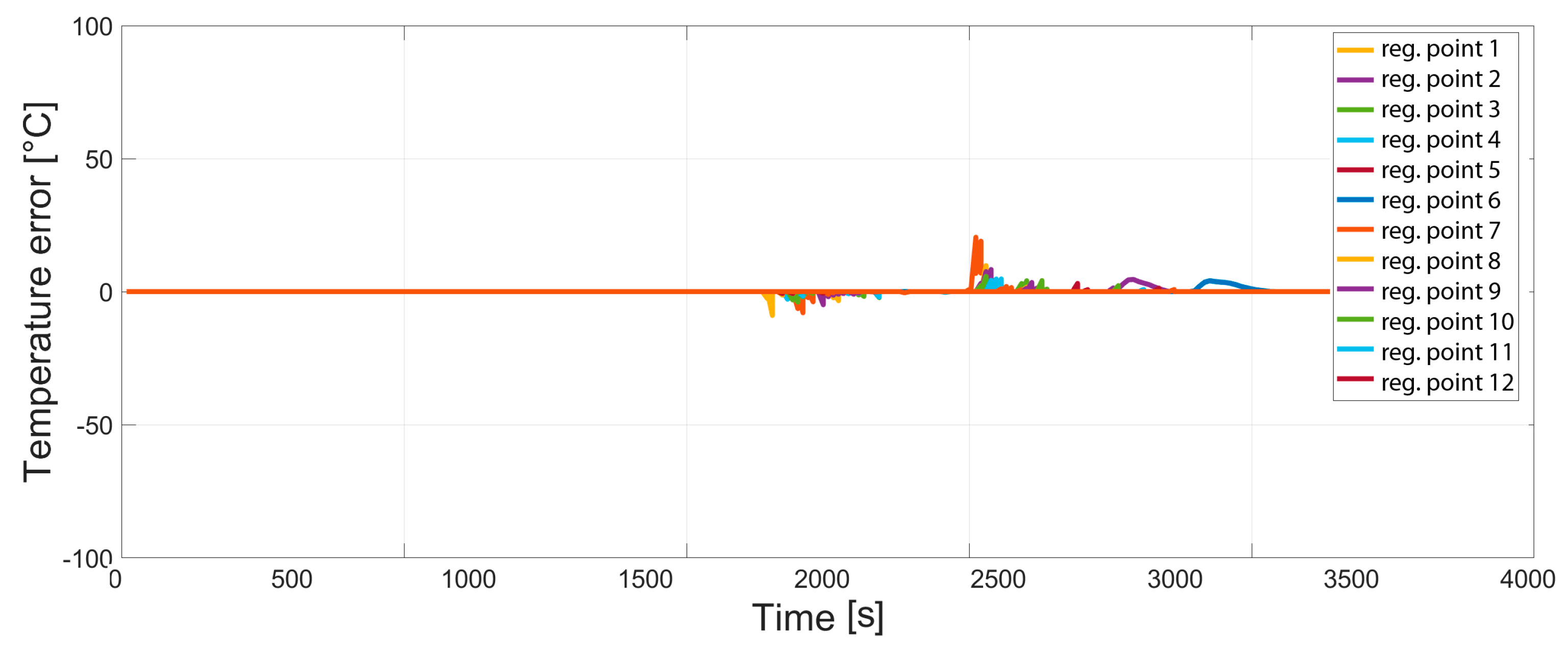
Another set of simulations were carried out for dynamic changes in process parameters such as casting speed or casting temperature. The following results show 1 h casting process where a drop of the casting speed from 1.9 to 1.2 m/min at time 30 min and the increase of the casting speed from 1.2 to 1.9 m/min occurs at time 40 min. The Figure 9 shows the response in cooling intensities for all 12 cooling loops on casting speed drop calculated by FL regulator. Because MPC were used, several future scenarios were calculated and optimal dynamic changes were found. The value of temperature errors after each regulation points (surface temperatures after each cooling loop) are shown in Figure 10. The maximal temperature error was approximately 20 °C but average temperature error was less than 10 °C. This can be consider as a very good regulation results.
Static and dynamic simulations proved regulation possibilities of the presented FL-BrDSM solution. The computation time without GPU was 27.25 min for static and 47.20 min for dynamic simulation. With GPU approach, the computation time was less than 1 min and 2 min in case of dynamic simulation respectively. This declares that there is no problem to solve complex fine-mesh (more than 3 million nodes) 3D transient solidification models and their optimal regulation in the real time on the real CC machine.
7. Conclusions
The FL-BrDSM was tested for many different fuzzy parameters, for different casting temperatures and casting speeds constraints, for different caster and slab geometries and for different steel grades. This paper is focused on the quality improvement of the steel grade S355 and demonstration of the FL-BrDSM. The first part of the work was focused on detail description of solidification model and its GPU version. Than FL regulator was described. Last part of the work was statistical evaluation of real historical casting data for steel grade S355. The influence of the surface temperature at the straightening area to the occurrence of surface defects was statistically evaluated as significant. From the statistic results the optimal (recommended) temperature field was obtained and used as the input to the FL-BrDSM. For different casting speeds the optimal cooling intensities were found. The control of the CC process using recommended cooling curves can decrease the number of surface defects. The dynamic simulation shows real time regulation possibilities in the case of casting speed drop. The same approach can be applied for any grade of steel. The main advantage of the presented approach is a small number of evaluations before the optimal solution is reached and its overall versatility. This also allows for the on-line real-time regulation of a real CC process.
Author Contributions
Conceptualization, T.M. and J.S.; Methodology, J.S.; Software, T.M.; Validation, T.M. and J.S.; Formal Analysis, J.S.; Investigation, T.M.; Resources, T.M.; Data Curation, J.S.; Writing-Original Draft Preparation, T.M.; Writing-Review & Editing, T.M.; Visualization, T.M.; Supervision, J.S.; Project Administration, J.S.; Funding Acquisition, J.S.
Funding
This research was funded by the project NETME+, LO1202, with the financial support from the Ministry of Education, Youth and Sports of the Czech Republic under the “National Sustainability Programme I and APC was funded by the Open Access fond Brno University of Technology.
Acknowledgments
The authors gratefully acknowledge funding from the Open Access fond Brno University of Technology and Specific research on BUT FSI-S-17-4444.
Conflicts of Interest
The authors declare no conflict of interest. The funders had no role in the design of the study; in the collection, analyses, or interpretation of data; in the writing of the manuscript and in the decision to publish the results.
References
- Flick, A.; Stoiber, C. Trends in continuous casting of steel: Yesterday, today and tomorrow. In Proceedings of the METEC InSteelCon, Düsseldorf, Germany, 27 June–1 July 2011; pp. 80–91. [Google Scholar]
- Birat, P.; Chow, C.; Emi, T.; Emling, W.H.; Fastert, H.P.; Fitzel, H.; Flemings, M.C.; Gaye, H.R.; Gilles, H.L.; Glaws, P.C.; et al. The Making, Shaping and Treating of Steel: Casting Volume, 11th ed.; The AISE Steel Foundation: Pittsburgh, PA, USA, 2003; p. 1000. ISBN 978-0-930767-04-4. [Google Scholar]
- Santos, C.A.; Spim, J.A.; Garcia, A. Mathematical modeling and optimization strategies (genetic algorithm and knowledge base) applied to the continuous casting of steel. Eng. Appl. Artif. Intell. 2003, 16, 511–527. [Google Scholar] [CrossRef]
- Zhemping, J.; Wang, B.; Xie, Z.; Lai, Z. Ant Colony Optimization Based Heat Transfer Coefficient Identification for Secondary Cooling Zone of Continuous Caster. In Proceedings of the IEEE International Conference Industrial Technology, Shenzhen, China, 20–24 March 2007; pp. 558–562. [Google Scholar] [CrossRef]
- Zheng, P.; Guo, J.; Hao, X.-J. Hybrid Strategies for Optimizing Continuous Casting Process of Steel. In Proceedings of the IEEE International Conference Industrial Technology, Hammamet, Tunisia, 8–10 December 2004; pp. 1156–1161. [Google Scholar] [CrossRef]
- Mauder, T.; Novotny, J. Two mathematical approaches for optimal control of the continuous slab casting process. In Proceedings of the Mendel 2010—16th International Conference on Soft Computing, Brno, Czech Republic, 26–28 June 2010; pp. 395–400, ISBN 978-80-214-4120-0. [Google Scholar]
- Ivanova, A.A. Predictive Control of Water Discharge in the Secondary Cooling Zone of a Continuous Caster. Metallurgist 2013, 57, 592–599. [Google Scholar] [CrossRef]
- Rao, R.V.; Kalyankar, V.D.; Waghmare, G. Parameters optimization of selected casting processes using teaching-learning-based optimization algorithm. Appl. Math. Modell. 2014, 38, 5592–5608. [Google Scholar] [CrossRef]
- Mosayebidorcheh, S.; Bandpy, M.G. Local and averaged-area analysis of steel slab heat transfer and phase. change in continuous casting process. Appl. Thermal Eng. 2017, 118, 724–733. [Google Scholar] [CrossRef]
- Mauder, T.; Charvat, P.; Stetina, J.; Klimes, L. Assessment of Basic Approaches to Numerical Modeling of Phase Change Problems-Accuracy, Efficiency, and Parallel Decomposition. J. Heat Transf. 2017, 139, 5. [Google Scholar] [CrossRef]
- Miettinen, J. IDS Solidification Analysis Package for Steels: User Manual of DOS Version 2.0.0; Helsinki University of Technology: Helsinki, Finland, 1999; p. 22. ISBN 9512246600. [Google Scholar]
- Zhang, J.; Chen, D.F.; Zhang, C.Q.; Wang, S.G.; Hwang, W.S.; Han, M.R. Effects of an even secondary cooling mode on the temperature and stress fields of round billet continuous casting steel. J. Mater. Process. Technol. 2015, 222, 315–326. [Google Scholar] [CrossRef]
- Javurek, M.; Ladner, P.; Watzinger, J.; Wimmer, P. Secondary cooling: Roll heat transfer during dry casting. In Proceedings of the METEC ESTAD, Düsseldorf, Germany, 15–19 June 2015; p. 8. [Google Scholar]
- Totten, G.E.; Bates, C.E.; Clinton, N.A. Handbook of Quenchants and Quenching Technology; Haddad, M.T., Ed.; ASM International: Materials Park, OH, USA, 1993; p. 507. ISBN 0-87170-448-X. [Google Scholar]
- Ramírez-López, A.; Muñoz-Negrón, D.; Palomar-Pardavé, M.; Romero-Romo, M.A.; Gonzalez-Trejo, J. Heat removal analysis on steel billets and slabs produced by continuous casting using numerical simulation. Int. J. Adv. Manuf. Technol. 2017, 93, 1545–1565. [Google Scholar] [CrossRef] [Green Version]
- Raudensky, M.; Hnizdil, M.; Hwang, J.Y.; Lee, S.H.; Kim, S.Y. Influence of Water Temperature on The Cooling Intensity of Mist Nozzles in Continuous Casting. Mater. Tehnol. 2012, 46, 311–315. [Google Scholar]
- Stetina, J.; Mauder, T.; Klimeš, L. Utilization of Nonlinear Model Predictive Control to Secondary Cooling during Dynamic Variations. In Proceedings of the AISTech, Pittsburgh, PA, USA, 16–19 May 2016; p. 14. [Google Scholar]
- Mauder, T.; Sandera, C.; Stetina, J. Optimal control algorithm for continuous casting process by using fuzzy logic. Steel Res. Int. 2015, 86, 785–798. [Google Scholar] [CrossRef]
- Louhenkilpi, S.; Laine, J.; Miettinen, J.; Vesanen, R. New Continuous Casting and Slab Tracking Simulators for Steel Industry. Mater. Sci. Forum 2013, 762, 691–698. [Google Scholar] [CrossRef]
Figure 1.
Scheme of the continuous casting and mechanical stresses during bending and straightening. 1—tundish; 2—mould; 3—nozzle; 4—cooling circuit; 5—roller.
Figure 1.
Scheme of the continuous casting and mechanical stresses during bending and straightening. 1—tundish; 2—mould; 3—nozzle; 4—cooling circuit; 5—roller.

Figure 2.
Temperatures and metallurgical length for different mesh densities.

Figure 3.
Numerical mesh CPU-GPU decomposition.

Figure 4.
Optimal temperature intervals.
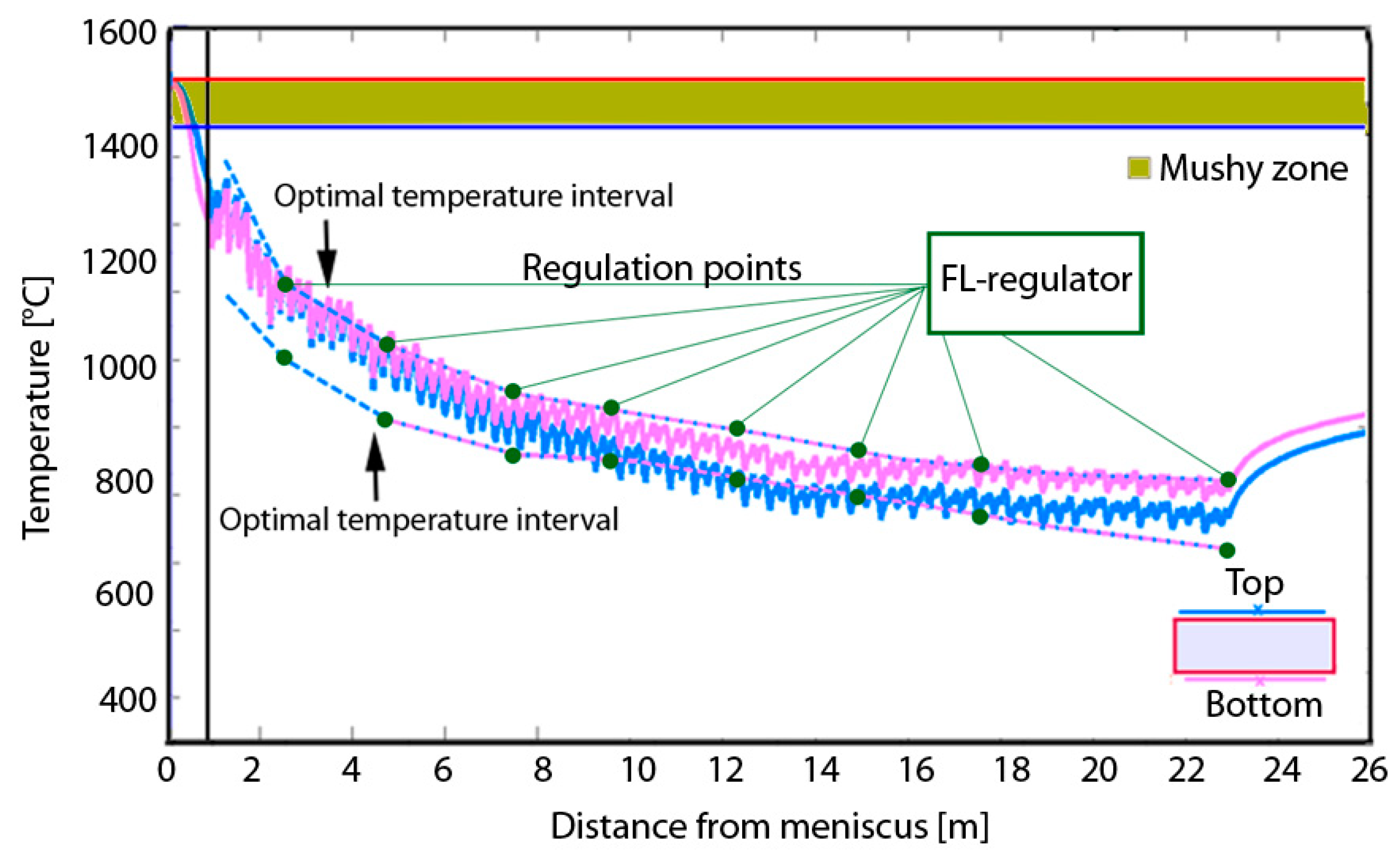
Figure 5.
Surface temperatures in unbending point with and without defects.
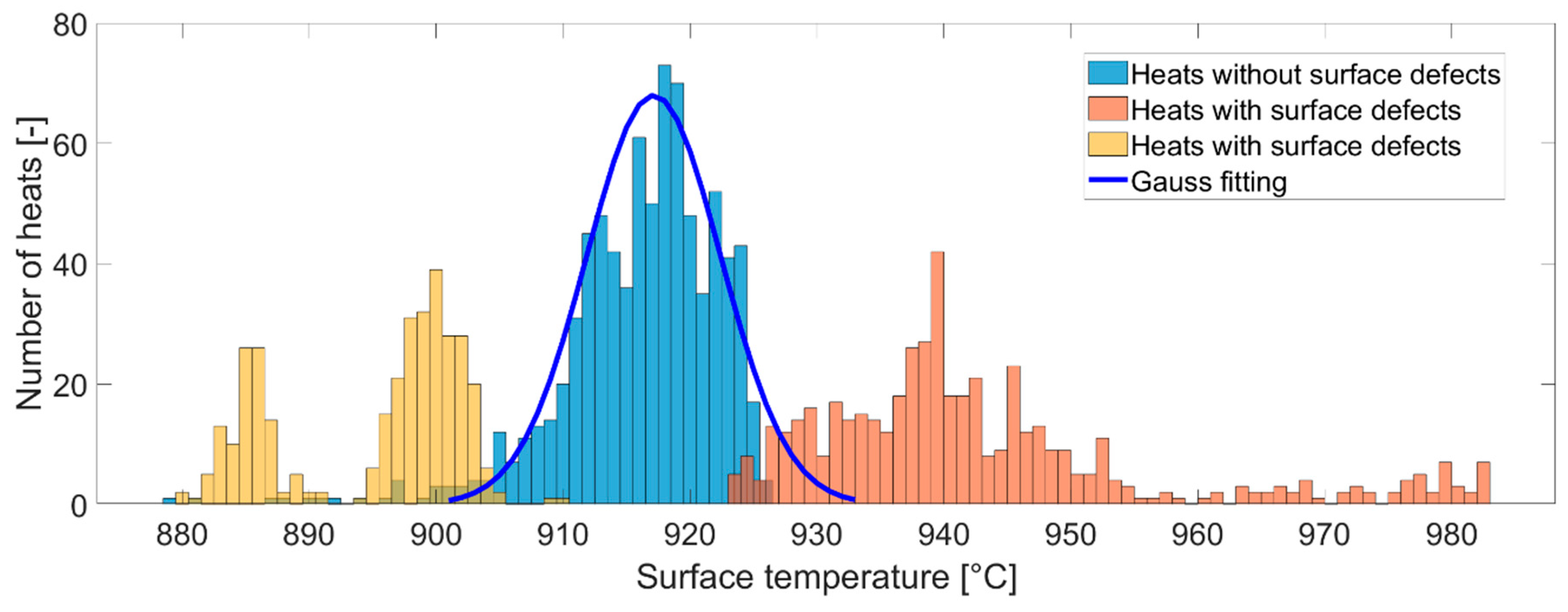
Figure 6.
Temperature dependent physical properties for the steel grade S355, (a) thermophysical properties; (b) Mechanical properties.
Figure 6.
Temperature dependent physical properties for the steel grade S355, (a) thermophysical properties; (b) Mechanical properties.
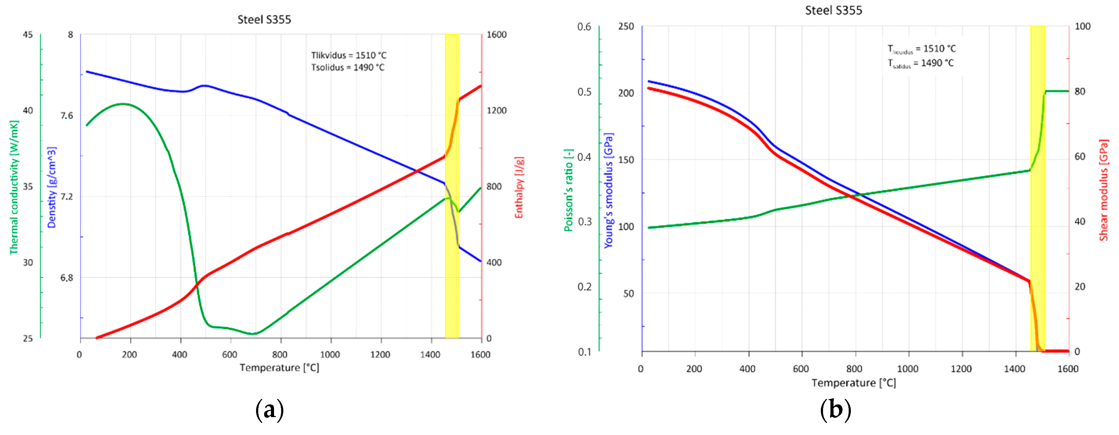
Figure 7.
Position of cooling loops.
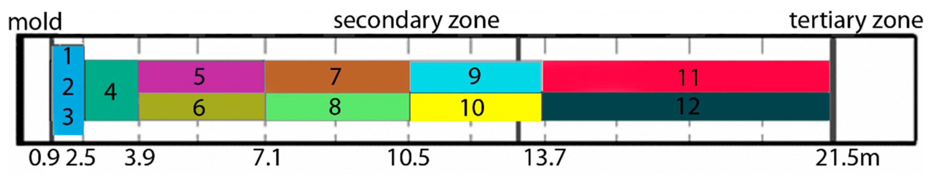
Figure 8.
Optimal temperature field after fuzzy regulation.
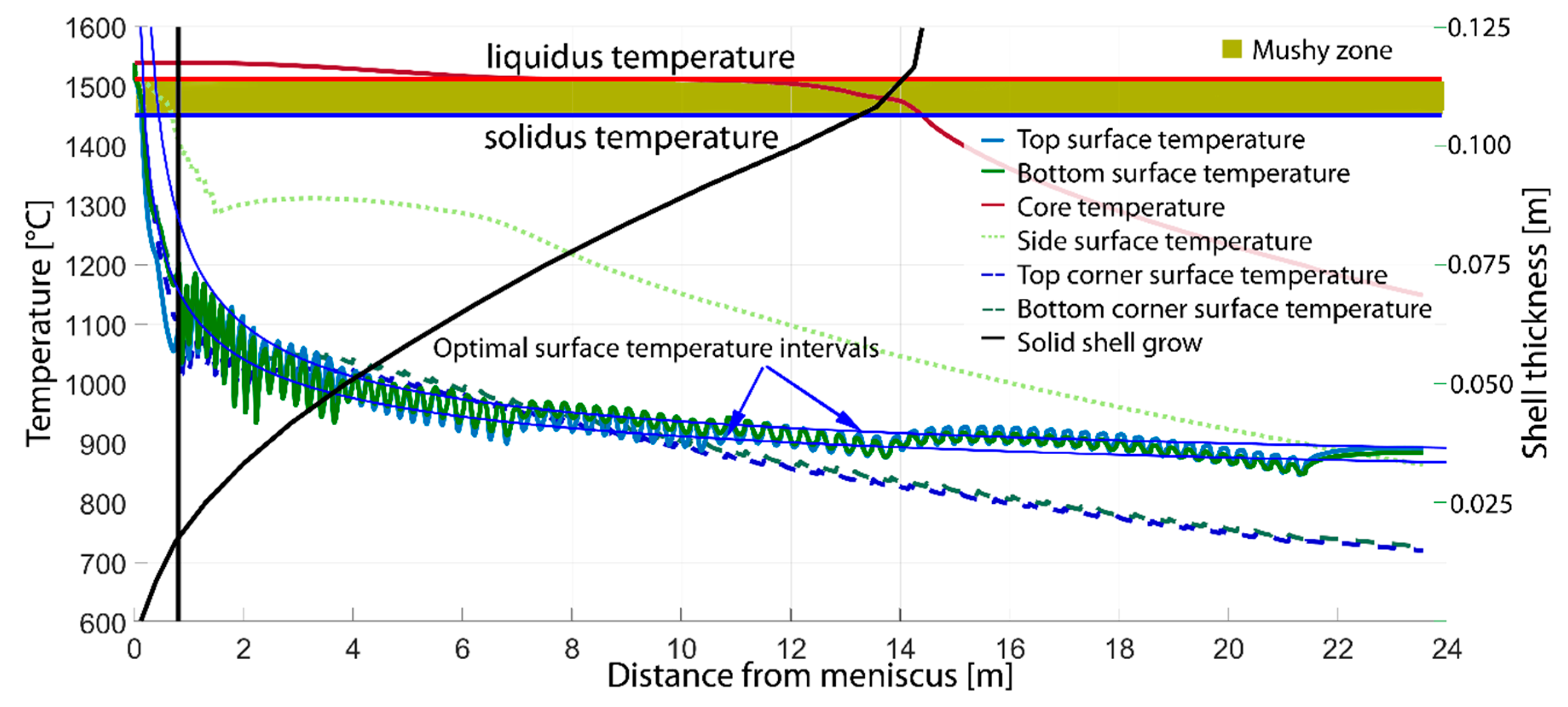
Figure 9.
Dynamic response of FL regulator to casting speed drop.

Figure 10.
Surface temperature errors after each cooling loop.

Table 1.
Computation time for non-parallel and parallel solution (s).
| Numerical Scheme | Computational Time (s) | ||
|---|---|---|---|
| Coarse mesh | Fine-mesh | Very-fine mesh | |
| SE—1 CPU | 11.54 | 887.14 | 54,362.12 |
| SE—12 CPU | 135.28 | 1122.13 | 35,124.54 |
| ADI—1 CPU | 41.81 | 714.73 | 36,210.41 |
| ADI—12 CPU | 58.61 | 824.32 | 32,416.32 |
| SE—GPU | 18.67 | 97.72 | 972.49 |
Table 2.
Chemical composition of steel S355.
| Weight Fraction | Ni | Mn | Mo | Si | Nb | Ti | Cu |
| wt% | max 0.300 | 1.400–1.550 | max 0.080 | 0.5 | max 0.060 | max 0.020 | max 0.200 |
| Weight Fraction | V | Al | P | C | Cr | S | Ca |
| wt% | max 0.020 | 0.020–0.060 | 0.030 | 0.160–0.180 | max 0.200 | 0.020 | 0.002 |
Table 3.
Optimal cooling intensities for cooling loops and different casting speeds.
| Casting Speed (m/min) | Loop 1 (L/min) | Loop 2 (L/min) | Loop 3 (L/min) | Loop 4 (L/min) | Loop 5 (L/min) | Loop 6 (L/min) |
| 1.5 | 96.6 | 125.4 | 103.9 | 124.6 | 65.3 | 98.5 |
| 1.9 | 98.1 | 132.6 | 109.5 | 146.3 | 98.3 | 103.3 |
| Casting Speed (m/min) | Loop 7 (L/min) | Loop 8 (L/min) | Loop 9 (L/min) | Loop 10 (L/min) | Loop 11 (L/min) | Loop 12 (L/min) |
| 1.5 | 32.0 | 65.7 | 22.0 | 34.7 | 31.2 | 43.7 |
| 1.9 | 46.9 | 85.7 | 26.7 | 58.3 | 99.5 | 106.2 |
© 2018 by the authors. Licensee MDPI, Basel, Switzerland. This article is an open access article distributed under the terms and conditions of the Creative Commons Attribution (CC BY) license (http://creativecommons.org/licenses/by/4.0/).
Share and Cite
MDPI and ACS Style
Mauder, T.; Stetina, J. High Quality Steel Casting by Using Advanced Mathematical Methods. Metals 2018, 8, 1019. https://doi.org/10.3390/met8121019
AMA Style
Mauder T, Stetina J. High Quality Steel Casting by Using Advanced Mathematical Methods. Metals. 2018; 8(12):1019. https://doi.org/10.3390/met8121019
Chicago/Turabian StyleMauder, Tomas, and Josef Stetina. 2018. "High Quality Steel Casting by Using Advanced Mathematical Methods" Metals 8, no. 12: 1019. https://doi.org/10.3390/met8121019
Note that from the first issue of 2016, this journal uses article numbers instead of page numbers. See further details here.