An Accurate Constitutive Model for AZ31B Magnesium Alloy during Superplastic Forming

Abstract

Accurate constitutive material models are essential for the realistic simulation of metal forming processes. However, for superplastic forming, mostly the material models found in the literature are based on fitting of the simple power law equation. In this study, an AZ31B constitutive model that takes into account microstructural evolution is introduced. This model takes into account grain growth and cavity formation in addition to strain and strain rate hardening. The model parameters were calibrated using the results of high temperature bulge forming tests and microstructural analysis. The Taguchi optimization method was used in the fitting process. In order to verify the model, simulations of the superplastic forming of two different geometries were carried out, and the results were compared with those obtained experimentally. Results show that the proposed model can accurately predict the formed geometry and thickness distribution.

1. Introduction

The ability of certain materials, under certain conditions, to undergo large uniform plastic strains is known as “superplasticity”. This phenomenon had been applied in the manufacturing of the Damascus steels from 300 B.C. to the late nineteenth century [1,2,3]. However, it was not before the sixties of the twentieth century that it was commercially re-applied in modern industrial applications. Currently, superplastic forming is used for manufacturing lightweight complex components in niche applications; such as in the aerospace, luxury and sports cars, trains, and medical industries.

Magnesium (Mg) alloys have many advantages, such as high specific strength and specific stiffness, excellent thermal conductivity, outstanding shock absorption, and strong electromagnetic shielding. However, because of their typical hexagonal close packed crystal structure, they exhibit low ductility at Room Temperature (RT), making their sheet applications greatly limited. However, the Mg alloy AZ31B, which possess superplastic properties, has been demonstrated to exhibit improved formability at warm and high temperatures [4,5]. Therefore, it can be used in forming parts without the need for secondary joining operations. In fact, complex parts in a near-net shape can be manufactured with this alloy. Achieving its full potential will create a wide range of new applications in the electronics, transportation, aerospace and other industries. Therefore, there is a great practical significance in studying the superplastic formability of AZ31B. This is particularly important for the aerospace and space applications, in which lightweight structuring is a major requirement.

Despite the potential of this alloy, it is a known fact that, there are only a small number of available experimental and numerical studies on the forming of AZ31B. Most of the constitutive models predicting the deformation of this alloy are oversimplified, based on tensile experiments, or not validated with enough experimental results.

When incorporated in the simulation of superplastic forming (SPF), the simple material models were reported to produce unsatisfactory results [6,7,8,9,10]. The main reason many studies rely on simple material models is the difficulty in determining the material constants. Over the years, several procedures have been introduced in the literature. For constitutive models with only two material constants, the least square method is usually used in establishing the unknown parameters. However, for constitutive models involving more than two material parameters, more sophisticated tools should be used. For example, the Taguchi method is a recently new powerful tool to optimize multiple parameters in experimental design. The utilization of such a tool in constitutive modeling has been proven to provide significant benefits in material modeling.

Furthermore, uniaxial tensile data has been used in superplastic constitutive modeling in a number of studies, see for example [10]. However, forming experiments has shown that such an approach would produce inaccurate results. This is expected because the stress state in uniaxial testing does not represent the conditions during the forming of actual components. In fact, bulge forming data are better to be used when modeling the SPF process [11].

Whereas, many studies have been carried out related to the constitutive modeling of the superplastic aluminum alloy AA5083, only a few studies were concerned with the Mg alloy AZ31B. Therefore, there is a need for an accurate constitutive model for this material. In this study, a new model was proposed for AZ31B that take into account the microstructure evolution during deformation. Furthermore, a new numerical-experimental procedure was proposed and followed for establishing the material parameters. A successful AZ31B model can contribute to the literature enormously.

2. Materials and Methods

The superplastic Mg alloy AZ31B is known to exhibit high ductility at elevated temperatures and low strain rates. As an example of such ductility, Figure 1 shows a comparison between uniaxial AZ31B specimens tested at various temperatures. The tests were conducted at a constant cross head speed of 0.01 mm/s. The original specimen of the as-received (AR) material is shown at the top of the figure. The specimen tested at RT showed a percent elongation of only 15.3%. The specimens tested at 100 °C and 450 °C showed a percent elongation of 24.1% and 113.7%, respectively.

The experiments in this study were conducted using sheets of AZ31B. The chemical constituents of the as-received AZ31B alloy used in this study are shown in

Table 1. As-received AZ31 alloy sheet chemical constituents (from vendor).

Element	Mg	Al	Zn	Mn	Si	Cu	Fe	Be	Ca
Percentage (%)	95.451	3.19	0.81	0.334	0.02	0.05	0.005	0.1	0.04

.

2.1. High-Temperature Bulge Forming

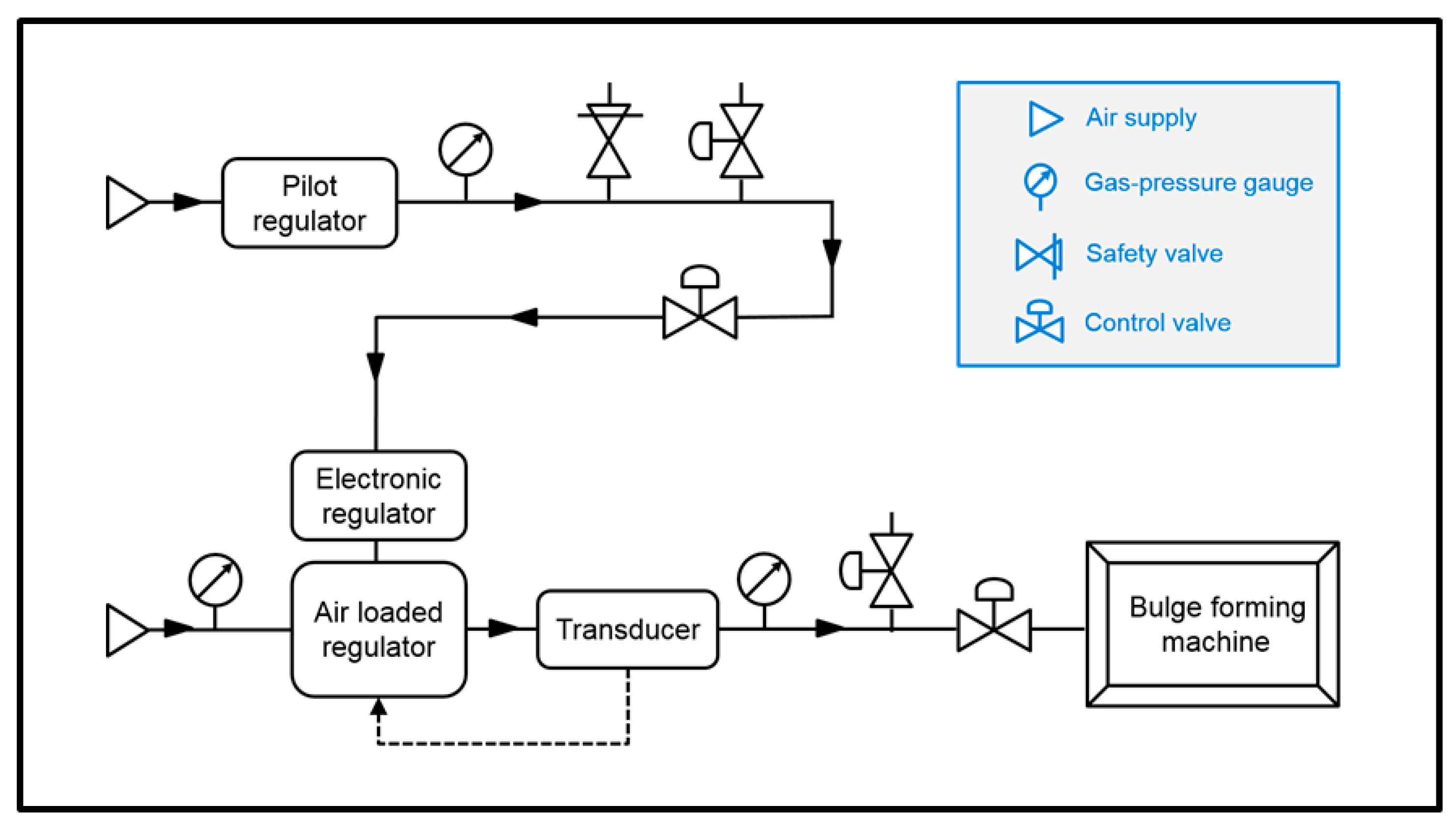
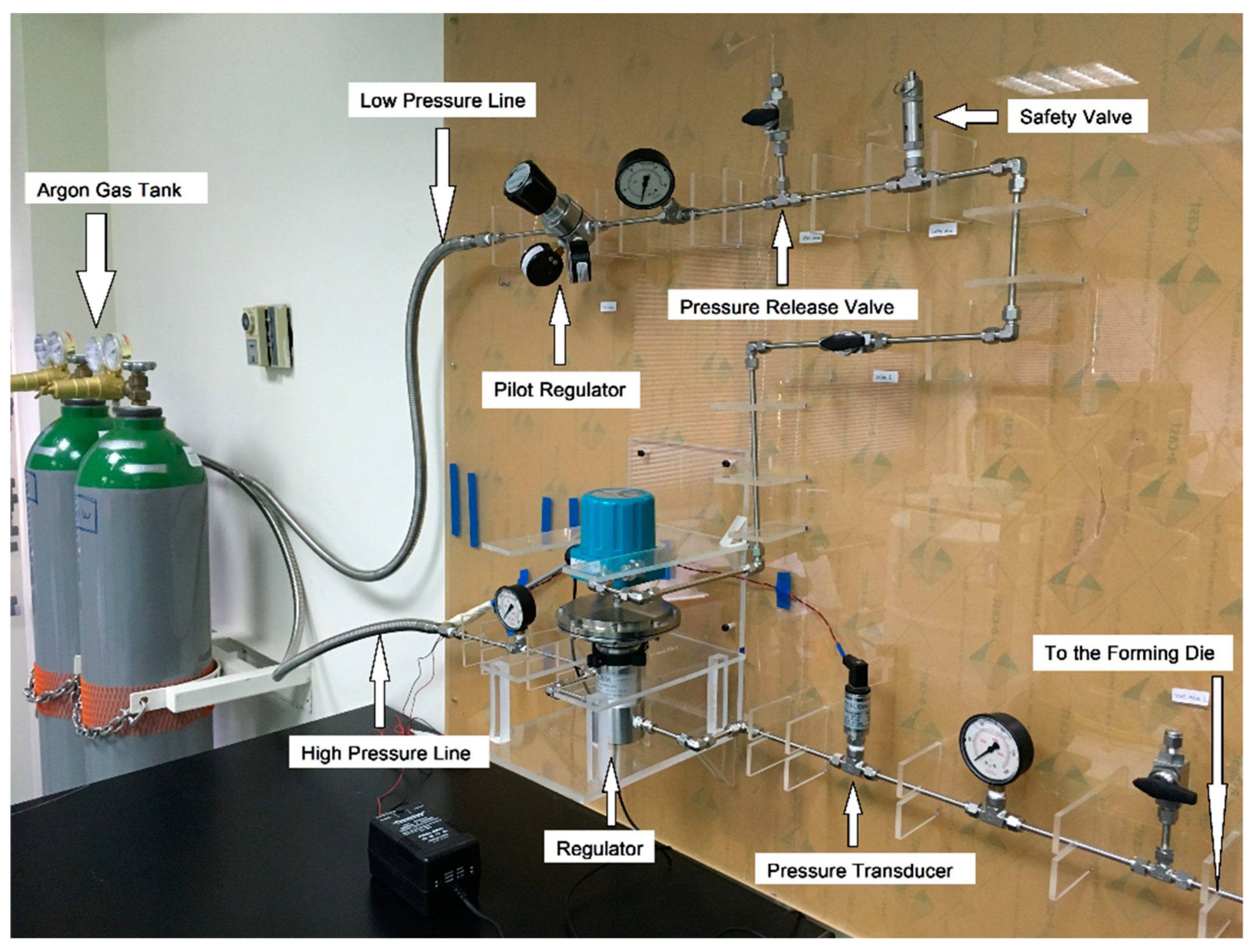
Since it resembles the initial stages in SPF of real components, high-temperature bulge forming is usually used for judging the formability of superplastic materials. In this study, an in-house developed SPF experimental setup, shown in Figure 2, was used for carrying out the bulge forming of AZ31B. The setup uses high pressure argon gas to blow the sheet specimen downwards into an open cylindrical die. The applied gas pressure is precisely controlled using the pressure control system, shown in Figure 2 and Figure 3. It contains two lines: A low pressure gas line and a high pressure one. For the low pressure line, a manual pressure reducing regulator (Pilot Regulator) is installed to limit the maximum pressure to 0.83 MPa. Gas from this line is used as input to an electronic regulator. The pressure output of the electronic regulator is tuned via a computer signal and is used to actuate an air loaded regulator. In the high pressure line, the pressure gets controlled using the air loaded regulator. In addition, a feedback transducer was added to improve the control precision of the system. Finally, the output from the high pressure line is used to perform the actual pneumatic forming.

Before applying the gas pressure, the die and the blank holder were both heated to a temperature of 450 °C by a ceramic band heater. According to recent studies by Sorgente et al. [12] and Kaya et al. [13], this temperature represents a valuable compromise between forming times, microstructure and formability. The 1.2 mm thick AZ31B sheet was then clamped between the die and the blank holder with force enough to seal the chamber between the blank holder and the sheet. It is assumed that the sheet will reach the forming temperature after clamping it for ten minutes.

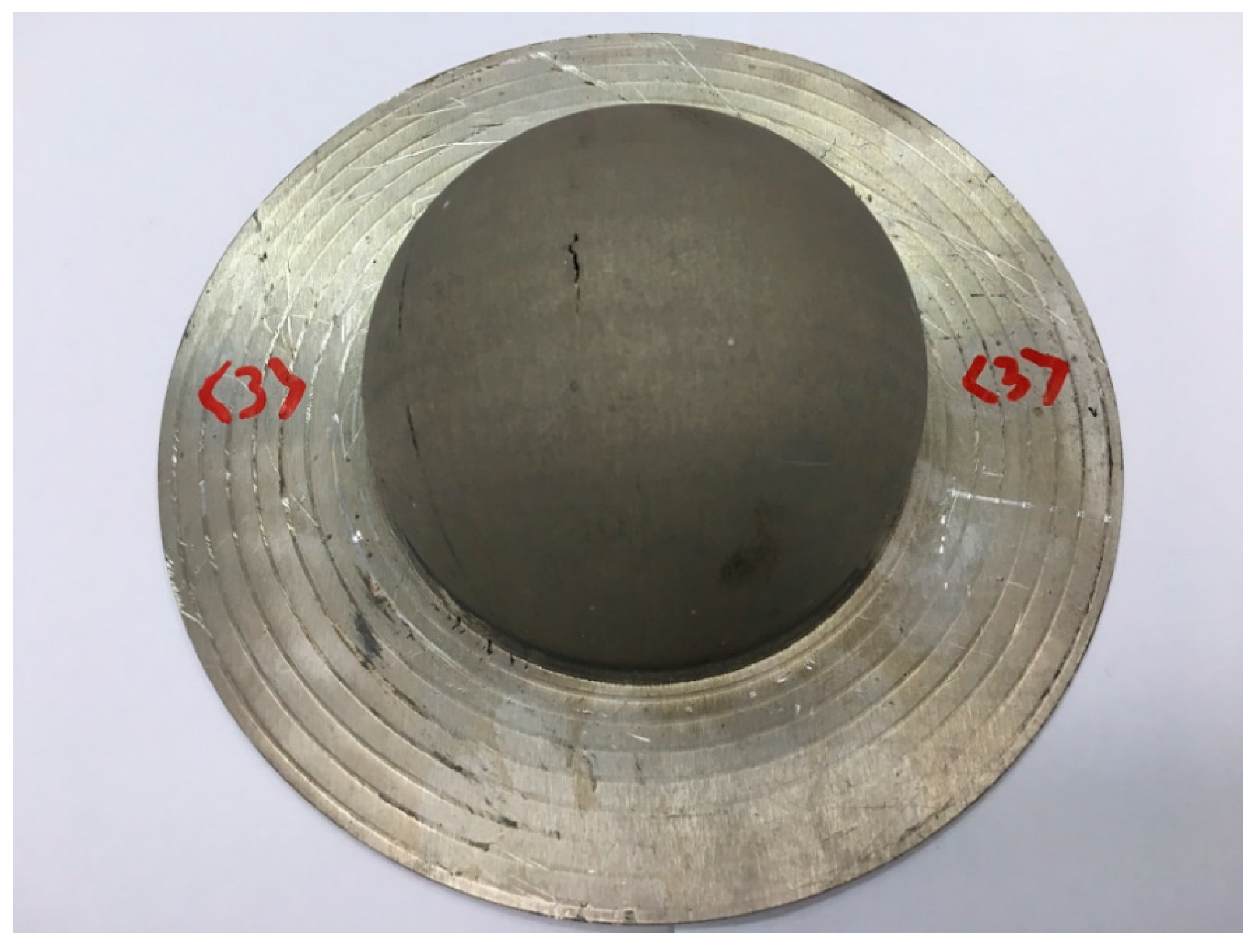
Bulge forming experiments were carried out, according to the ASTM E2712-15 standard [14], using constant gas pressures of 0.15, 0.2, and 0.3 MPa which are similar in magnitude to those considered by Franchitti et al. [15] for the same alloy. Furthermore, for each pressure, the rupture time of the AZ31B sheet was first determined by taking the average of three trials. Figure 4 shows an AZ31B sheet bulge formed up to rupture at a temperature of 450 °C and using a constant gas pressure of 0.15 MPa. Afterwards, the rupture time for each pressure level was divided into six intervals in order to determine the times at which to terminate the tests. At the end of each test, the specimen was removed and allowed to air cool to room temperature. The dome height was then recorded, and the specimen was cut into two halves for measuring the pole thickness. It is noteworthy that for each constant pressure and at each forming time three different trials were conducted. The complete results of the bulge forming experiments are shown in

Table 2. The measured dome height and pole thickness from bulge forming at a constant pressure of 0.15 MPa.

0.15 MPa
Measurements	1	2	3	Average Value
time (sec)	240.0	240.0	240.0	240.0
dome height (mm)	25.30	24.63	24.57	24.83
pole thickness (mm)	0.91	0.96	0.97	0.95
time (sec)	480.0	480.0	480.0	480.0
dome height (mm)	32.88	32.15	33.39	32.81
pole thickness (mm)	0.74	0.77	0.73	0.75
time (sec)	720.0	720.0	720.0	720.0
dome height (mm)	37.49	37.70	-	37.60
pole thickness (mm)	0.67	0.64	-	0.66
time (sec)	960.0	960.0	960.0	960.0
dome height (mm)	47.49	48.18	-	47.84
pole thickness (mm)	0.43	0.41	-	0.42
time (sec)	1200.0	1200.0	1200.0	1200.0
dome height (mm)	55.40	46.00	51.72	51.04
pole thickness (mm)	0.35	0.50	0.34	0.40
rupture time (sec)	1663.0	1433.0	1661.00	1585.7
dome height (mm)	57.66	60.30	59.71	59.22
pole thickness (mm)	0.43	0.35	0.39	0.39

,

Table 3. The measured dome height and pole thickness from bulge forming at a constant pressure of 0.2 MPa.

0.2 MPa
Measurements	1	2	3	Average Value
time (sec)	80.0	80.0	80.0	80.0
dome height (mm)	22.57	25.30	22.87	23.58
pole thickness (mm)	0.90	0.83	0.91	0.88
time (sec)	180.0	180.0	180.0	180.0
dome height (mm)	30.46	30.68	29.10	30.08
pole thickness (mm)	0.77	0.76	0.78	0.77
time (sec)	280.0	280.0	280.0	280.0
dome height (mm)	34.38	32.34	31.57	32.76
pole thickness (mm)	0.70	0.80	0.80	0.77
time (sec)	380.0	380.0	380.0	380.0
dome height (mm)	40.47	40.80	35.35	38.87
pole thickness (mm)	0.57	0.57	0.73	0.62
time (sec)	480.0	480.0	480.0	480.0
dome height (mm)	46.82	44.18	50.15	47.05
pole thickness (mm)	0.48	0.49	0.40	0.46
rupture time (sec)	580.0	-	619.0	599.5
dome height (mm)	45.70	-	51.41	48.56
pole thickness (mm)	0.49	-	0.40	0.45

and

Table 4. The measured dome height and pole thickness from bulge forming at a constant pressure of 0.3 MPa.

0.3 MPa
Measurements	1	2	3	4	Average Value
time (sec)	30.00	30.00	30.00	30.00	30.00
dome height (mm)	26.46	23.89	26.35	24.02	25.18
pole thickness (mm)	0.73	0.86	0.71	0.91	0.80
time (sec)	60.00	60.00	60.00	60.00	60.00
dome height (mm)	27.49	31.08	25.50	32.07	29.04
pole thickness (mm)	0.77	0.66	0.83	0.69	0.74
time (sec)	90.00	90.00	90.00	-	90.00
dome height (mm)	31.65	33.10	28.93	-	31.23
pole thickness (mm)	0.67	0.60	0.76	-	0.68
time (sec)	120.00	120.00	120.00	-	120.00
dome height (mm)	46.02	40.12	40.94	-	42.36
pole thickness (mm)	0.44	0.56	0.52	-	0.51
rupture time (sec)	171.00	145.00	172.00	-	162.67
dome height (mm)	41.39	47.74	45.83	-	44.99
pole thickness (mm)	0.53	0.36	0.40	-	0.43

.

2.2. Microstructure Analysis

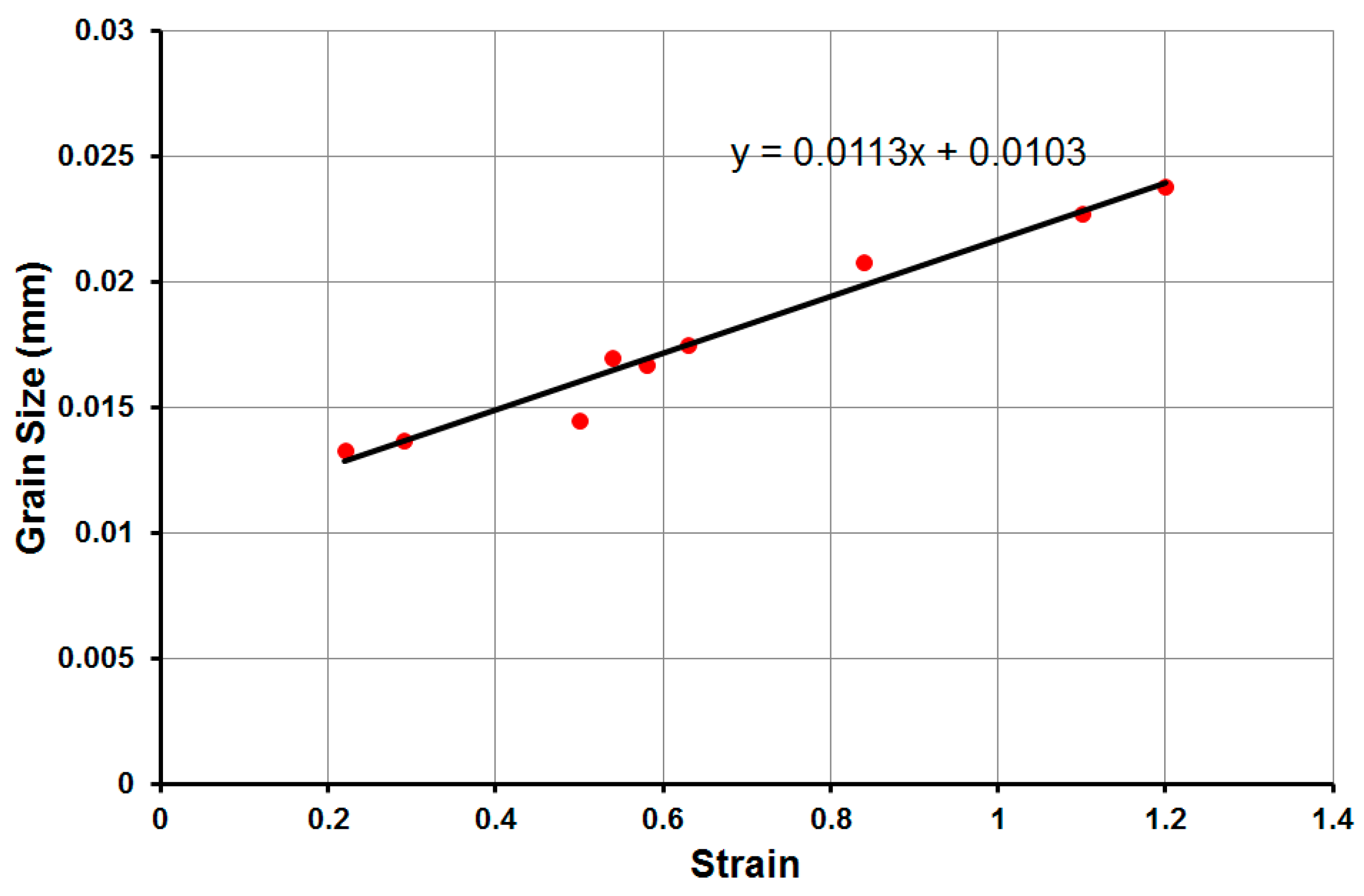
Samples were cut from the bulge formed specimens around the pole area. The samples were then prepared for optical microscopy using a 5 megapixel digital camera microscope (OLYMPUS DP27, MEA FZ-LLC, Dubai, United Arab Emirates). This was accomplished by a sequence of grinding and polishing steps followed by the application of acetic-picral as an etchant. Considering samples from forming under different pressures up to different times, a relationship was established between the grain size and the strain, as shown in Figure 5. When extrapolated, the linear relationship crosses the y-axis at a grain size of 10.3 micrometers. This value agrees with the typical required initial grain size for superplastic materials.

2.3. Constitutive Modeling

Accurate constitutive material models are essential for the realistic simulation of the SPF process. Many established models found in the literature are identified as phenomenological material models [6,7,8,9,10,16,17,18,19,20,21]. These are viscoplastic models that represent the macroscopic behavior of deformation, usually at a constant forming temperature. They reflect mainly the relationship between the effective flow stress and the effective strain and strain rate. The constants in these models are fitted using uniaxial tensile [10] or bulge forming experimental data [9,20,21].

The superplastic behavior in many cases is represented by the simple power law equation

$$\sigma =K{\dot{\epsilon }}^m$$

(1)

where ($\sigma$) is the effective flow stress, ($K$) is the material strength coefficient, ($\dot{\epsilon }$) is the effective strain rate, and ($m$) is the strain rate sensitivity index which should be greater than 0.3 for superplastic behavior to exist, and thus, the high sensitivity to strain rate.

As a first stage in establishing a material model for AZ31B, calibration of the constitutive in Equation (1) was carried out using data from the bulge forming experiments and following the procedure by Enikeev and Kruglov [22]. For two different pressures ($P_1$) and ($P_2$), the forming times ($t_1$) and ($t_2$) are defined as the corresponding forming times that lead to the same pole height ($h$). According to Reference [22] the value of ($m$) can be determined using the following equation:

$$m=\frac{\ln (P_1/P_2)}{\ln (t_2/t_1)}$$

(2)

A schematic representation of the free bulging process is shown in Figure 6. The angle ($\alpha$) is defined as half of the angle subtended by the dome surface at the center of curvature.

In this study, instead of relying only on two sets of data points ($P$, $t$), an averaged strain rate sensitivity index ($m$) was determined using six different values of ($\alpha$), see

Table 5. Calculation of an averaged strain rate sensitivity index using Equations (2) and (3).

Angle	P1 = 0.15 MPa		P2 = 0.2 MPa		m
α	h (mm)	t1 (sec)	h (mm)	t2 (sec)
53.1°	25.5	292	25.5	106	0.284
60°	29.45	382	29.45	170	0.355
66.7°	33.56	532	33.56	293	0.482
73.1°	37.8	720	37.8	346	0.393
79.1°	42.14	824	42.14	420	0.427
90°	51	1200	51	619	0.435

and

Table 6. The values of the material parameter ($K$) for the two considered pressures $P_1$ and $P_2$.

Angle	P1 = 0.15 MPa			P2 = 0.2 MPa
α	Im	t1 (sec)	K1	Im	t2 (sec)	K2
53.1°	0.0264	292	100.13	0.0264	106	89.01
60°	0.038	382	96.37	0.038	170	92.95
66.7°	0.0502	532	98.43	0.0502	293	103.38
73.1°	0.0619	720	102.16	0.0619	346	101.61
79.1°	0.0721	824	101.45	0.0721	420	103.30
90°	0.0874	1200	109.17	0.0874	619	111.7

. These correspond to six different values of the pole height ($h$) as calculated by the geometric relationship

$$h=R(1-\cos \alpha )=R_0(tan\frac{\alpha }{2})$$

(3)

where ($R_0=51 \mathrm{mm}$) is the die radius.

It is noteworthy that, in Table 5 and Table 6, the first experimental data corresponds to a value of ($\alpha \cong 53.1°$). This is due to the high rate of change in ($\alpha$) at the initial stages of the test, which limits the practicality of collecting data for ($\alpha <53.1°$).

From the data in Table 2, Table 3 and Table 4 and using the linear interpolation method, the forming times corresponding to the six values of the pole height were calculated for the constant pressures ($P_1=0.15 \mathrm{MPa}$) and ($P_2=0.2 \mathrm{MPa}$). Then Equation (2) was used to generate six different values of the strain rate sensitivity index ($m$). At last, an average value of 0.4 from the six distinct ($m$) values was obtained. A summary of these calculations is found in Table 5.

According to Reference [22], the parameter ($K$) is the average of ($K_1$) and ($K_2$) as calculated from the expressions:

$$K_i=\frac{P_i R_0}{2 S_0}{(\frac{t_i}{2 I_m(\alpha )})}^m, i=1,2,$$

(4)

$$I_m={\int }_0^{\alpha }{(\raisebox{1ex}{${sin}^{3}x$}\!\left/ \!\raisebox{-1ex}{$x^2$}\right.)}^{\frac{1}{m}} (\frac{1}{x}-\frac{1}{tanx})dx,$$

(5)

where ($S_0$) is the initial thickness of the sheet, which is equal to 1.2 mm. Actually, the integral on the right side of Equation (5) is not expressed through elementary functions; however, it can be easily calculated numerically. Table 6 shows the values of ($K_1$) and ($K_2$) calculated from Equations (4) and (5). An average value of the material strength coefficient ($K$) was determined to be $100 \mathrm{MPa}·{\sec }^m$. Notice that the model constants ($m$) and ($K$) were calculated directly with no need for any assumptions or trial and error.

Following is a relatively more sophisticated constitutive model that has been used in a number of studies [23,24,25,26] for superplastic materials. This model involves the effects of strain hardening, strain rate sensitivity, grain growth and cavitation:

$$\sigma =A(1-f_{ao}{e}^{\psi \epsilon }){(d_o+C\epsilon )}^n{\dot{\epsilon }}^m$$

(6)

where ($\epsilon$) is the effective strain, ($d_o$) is the initial grain size, ($f_{ao}$) is the initial area fraction of voids, ($\psi$) is the void growth index, ($n$) is strain hardening exponent, ($C$) is a grain growth constant, and ($A$) is a material constant. However, in the aforementioned studies [23,24,25,26], the values of the parameters were determined by trial and error.

In order to calibrate this model for the AZ31B material, the following procedure was carried out. The value of the strain rate sensitivity index ($m$) was taken to be the same as that calculated for the simple model Equation (1). The values of ($d_o$) and ($C$) were based on the relationship between the grain size and the strain established from the microstructure analysis. The strain hardening exponent ($n$) was assigned a value of 0.2, similar to its value in a previous study by Li et al. [27]. Since no experimental results were available on the volume fraction of voids, ($f_{ao}$) and ($\psi$), the values of (A, $f_{ao}$ and ψ) were determined using the Taguchi design method.

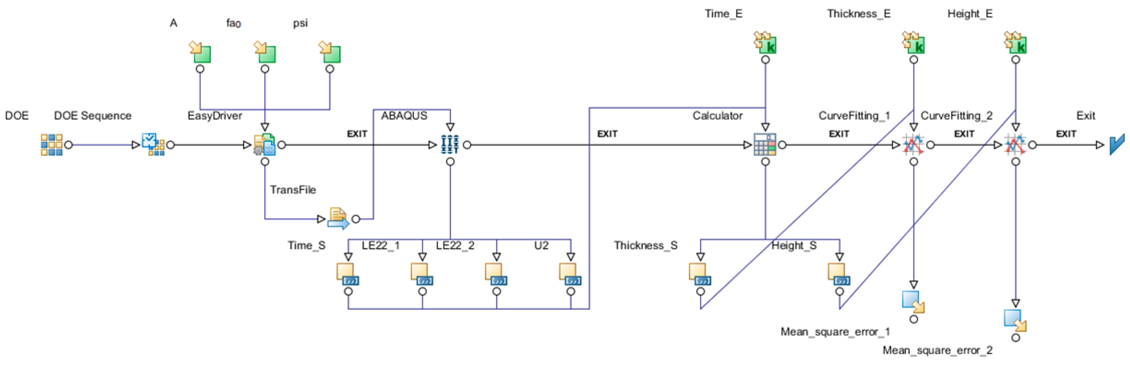
Taguchi method is a powerful tool to optimize multiple parameters in experimental design that produces the minimum experimental units [28,29,30]. This method was implemented in the commercially available optimization software modeFRONTIER version 2017R2 (ESTECO, AREA Science Park, Trieste, Italy). Figure 7 shows the workflow chart for the optimization of parameters ($A$, $f_{ao}$, and $\psi$). At first, a Design of Experiment (DOE) was set up, and the acceptable range for the three parameters was established.

An EasyDriver function was created with the input file, and the material Fortran-subroutine file for ABAQUS added to this EasyDriver. Parameter ($A$) was linked with the Fortran file, and EasyDriver performed the loop operations of ABAQUS version 6.13-1 (Dassault Systemes, Velizy-Villacoublay Cedex, France) simulations changing the value of ($A$) automatically.

When the loop operations were finished, the simulated output (ODB) files were imported into ABAQUS through the Transfile function, then the simulated time (Time-S), through thickness strain of the pole elements (LE22-1 and LE22-2) and vertical displacement of the same element (U2) were obtained from ABAQUS.

Time-S, LE22, and U2 were imported into the Calculator box, in which, the relationship between the simulation pole thickness (Thickness-S) and LE22 were defined, as well as for the relationship between the dome height (Height-S) and U2. Then the simulation-generated pole thickness and dome height corresponding to the experimental time (Time-E) were obtained through interpolation.

Finally, the mean square error (MSE) of the pole thickness was calculated by comparing the Thickness-S with experimental pole thickness (Thickness-E) through a (CurveFitting-1) function. The MSE of the dome height (Mean-square-error-2) was obtained by comparing the Thickness-H with the experimental dome height (Height-E) through CurveFitting-2.

In the first round of optimization, the acceptable ranges for the parameters ($A$), ($f_{ao}$) and ($\psi$) were set as 100–500, 0.01–0.1, and 0–1.8, respectively. An arbitrary combination of the values of ($A$), ($f_{ao}$) and ($\psi$) were set in 30 different simulated experiments. Figure 8 shows the MSE of both the pole thickness and dome height corresponding to different values of the parameter ($A$) at P = 0.15 MPa. From the figure, it can be concluded that the optimum value of ($A$) is roughly in the range of 230 to 320. The corresponding figures for ($f_{ao}$) and ($\psi$) were not conclusive.

The second round of optimization was carried out with the range of parameter ($A$) reduced to 230-320. The ranges of parameters ($f_{ao}$) and ($\psi$) were still 0.01–0.1 and 0–1.8, respectively. The step sizes for the parameters ($A$), ($f_{ao}$) and ($\psi$) were 10, 0.01 and 0.2, respectively. For a conventional Design of Experiment (DOE), 1000 simulations need to be performed to achieve the optimum values for the three parameters, because parameter ($A$), ($f_{ao}$) and ($\psi$) have 10 different values, respectively. However, the number of experiment sets was decreased to 100 through the use of the Taguchi method. The three parameters were arrayed orthogonally using the Taguchi method. A total of 100 simulations were conducted for the three different pressures (0.15 MPa, 0.2 MPa and 0.3 MPa).

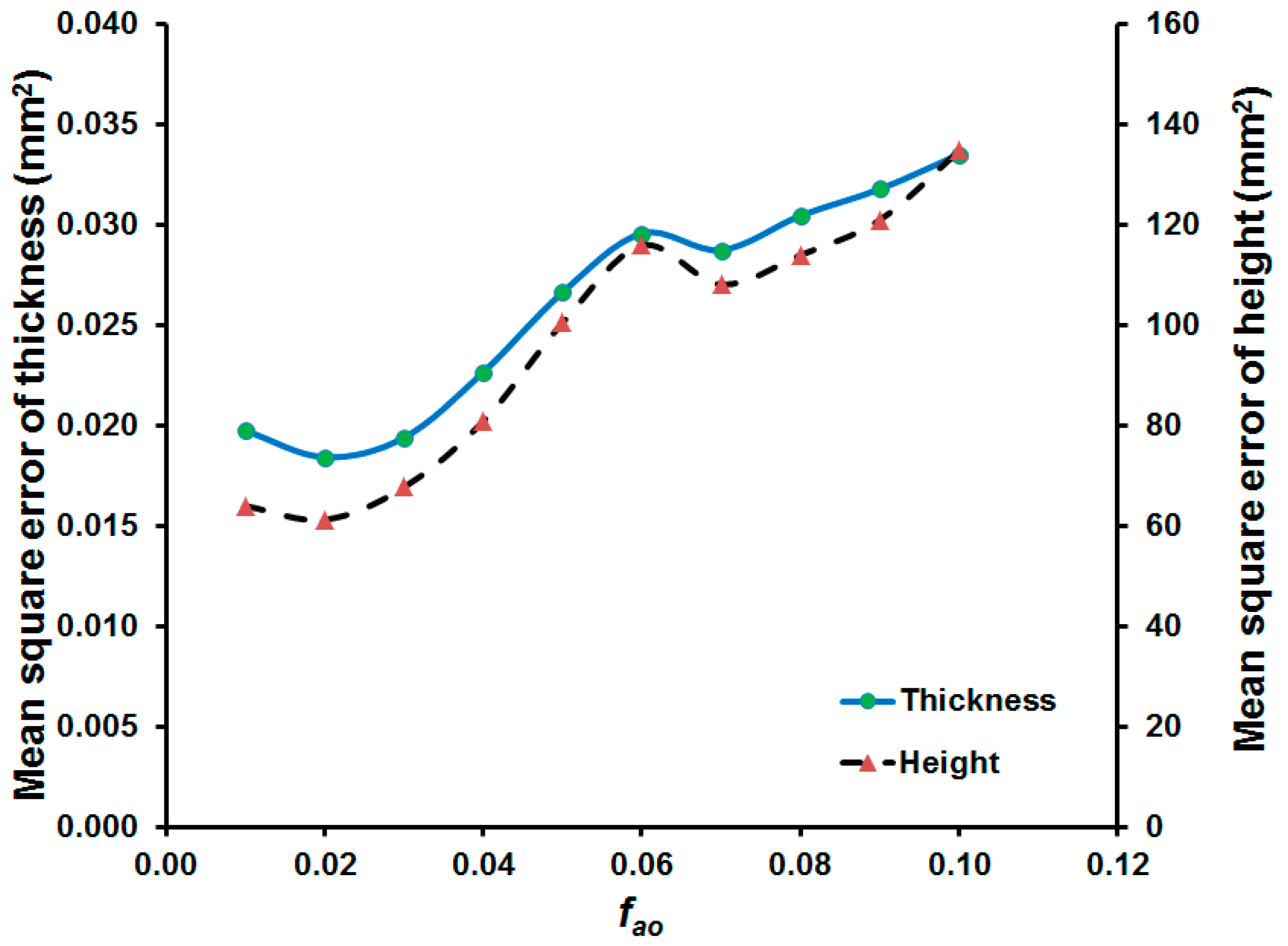
Figure 9 demonstrates the influence of ($f_{ao}$) on the MSE of the pole thickness and dome height for P = 0.15 MPa. Both the pole thickness and dome height almost have the same trend with a minimum value of MSE at ($f_{ao}$ = 0.02). Corresponding to the results considering the pressure values of 0.2 MPa and 0.3 MPa, not shown here for briefness, a final average value of 0.01 was set for ($f_{ao}$).

Figure 10 displays the influence of ($\psi$) on the MSE of the pole thickness and the dome height for a forming pressure of 0.15 MPa. An optimum value of ($\psi$) of 0.6 can be easily identified from the figure. Almost the same result was obtained for P = 0.2 MPa and P = 0.3 MPa.

Figure 11 shows the effect of ($A$) on the MSE of the pole thickness and dome height for P = 0.15 MPa. For this pressure value, from the figure, the optimum value of ($A$) is around 280. The optimum of ($A$) was about 270 for P = 0.2 MPa and in the range between 260 and 270 for P = 0.3 MPa. The range of parameter ($A$) was further narrowed down with the third round of optimization.

For the last round of optimization, the values of ($f_{ao}$) and ($\psi$) were fixed to 0.01 and 0.6, respectively. The range of parameter ($A$) was chosen to be between 245 and 280 for the three pressures. After running the analysis, the optimum value of parameter ($A$) was found to be 256. Therefore, the final obtained form of the AZ31B material model is given by

$$\sigma =256(1-0.01e^{0.6\epsilon }){(0.0103+0.0113\epsilon )}^{0.2}{\dot{\epsilon }}^{0.4}.$$

(7)

3. Results and Discussion

3.1. SPF a Cup with a Cylindrical Boss

The goal here is to form an AZ31B part with a primary and a secondary feature. Figure 12 shows a three-dimensional representation of this relatively complicated part. It consists of a cup (a primary feature) with a cylindrical boss (a secondary feature) at its base. It is needless to say that this component is difficult to form using conventional forming techniques. To produce this part, a closed die with an inner cavity was used. The surface of the inner cavity has the same geometry as the desired shape of the finished part. Figure 13 shows a finished part after 40 min of SPF using a constant gas pressure of 0.15 MPa.

The constitutive model developed in the previous section was incorporated in a finite element analysis carried out using ABAQUS. An axisymmetric model was used for the simulation of the SPF of the part that is shown in Figure 14. The 102-mm diameter circular die with a die entry radius ER of 3 mm was modeled as a rigid analytical surface. The 1.2-mm thick sheet was modeled using four layers of axisymmetric elements. Each layer contained 300 solid elements. The sheet elements between the die and the blank holder were assumed to be fixed. This was necessary in order to simulate the pure stretching condition in the SPF process. Since no lubricant was used in the actual forming, a coefficient of coulomb friction of 0.8 at the die-sheet interface was considered in the simulations [24]. The height of the boss (h) is 6 mm. The diameters of the boss are 22.8 mm and 40.6 mm for (d₁) and (d₂), respectively. (R₁) and (R₂) is 3.6 mm and 6 mm, respectively.

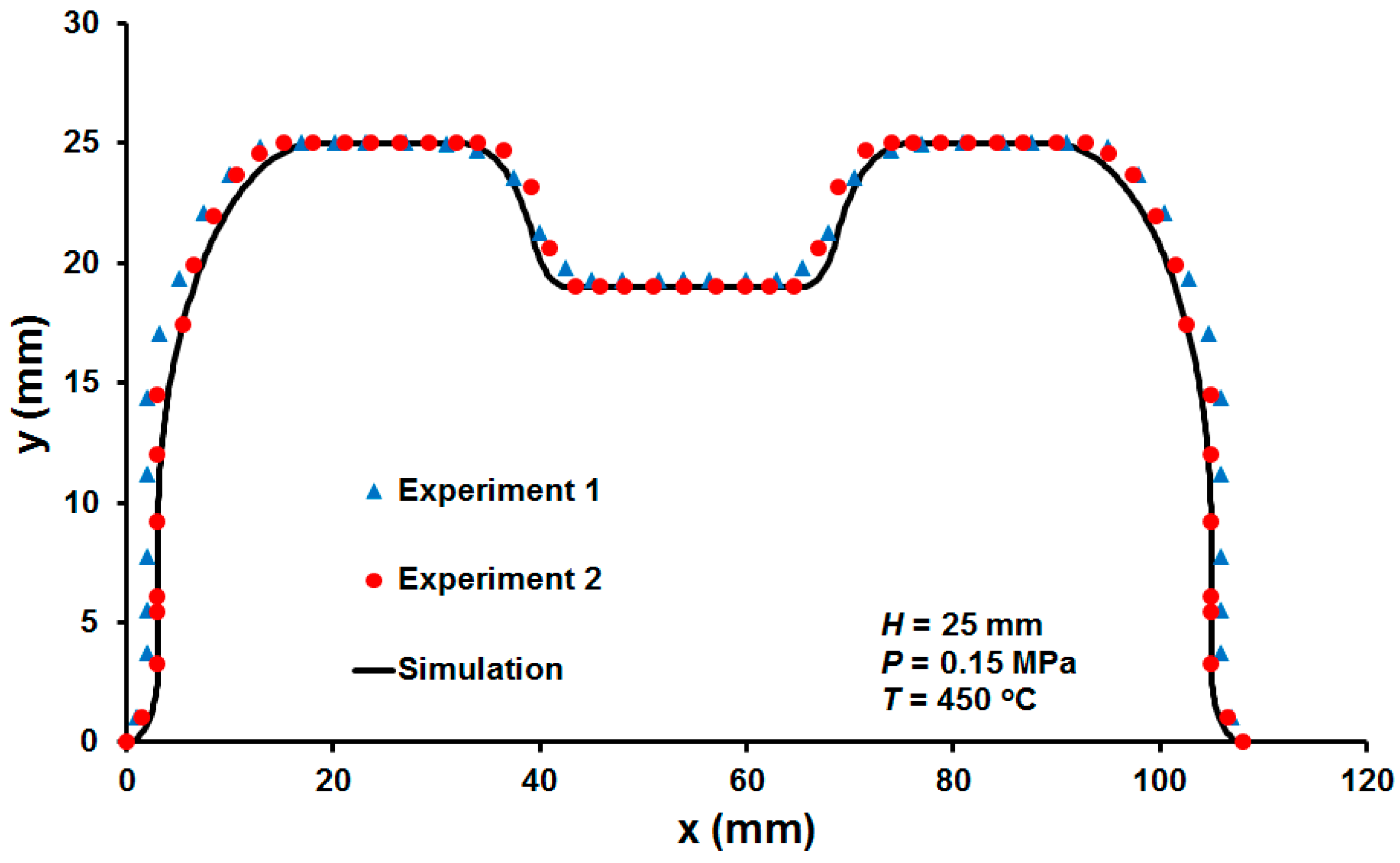
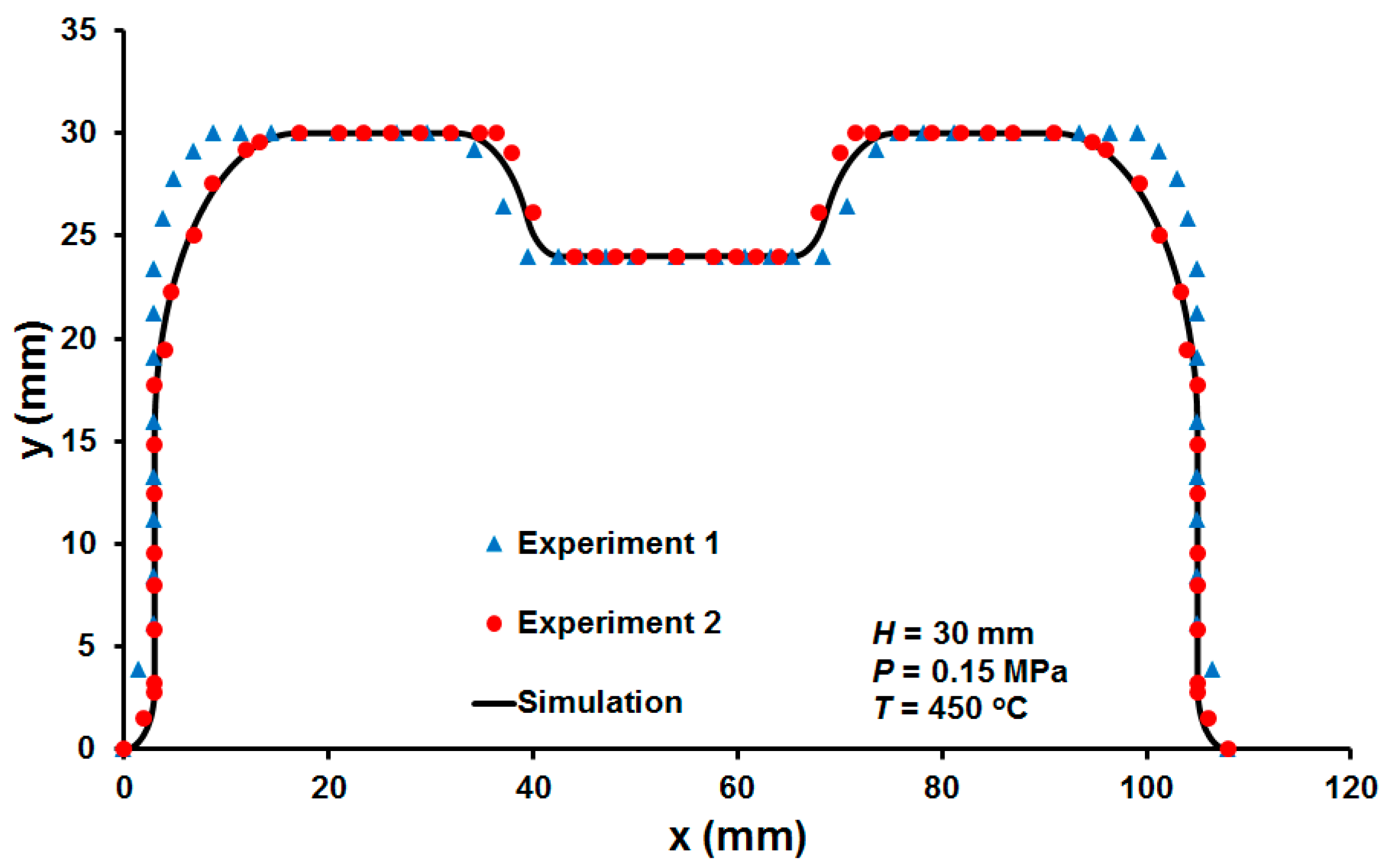
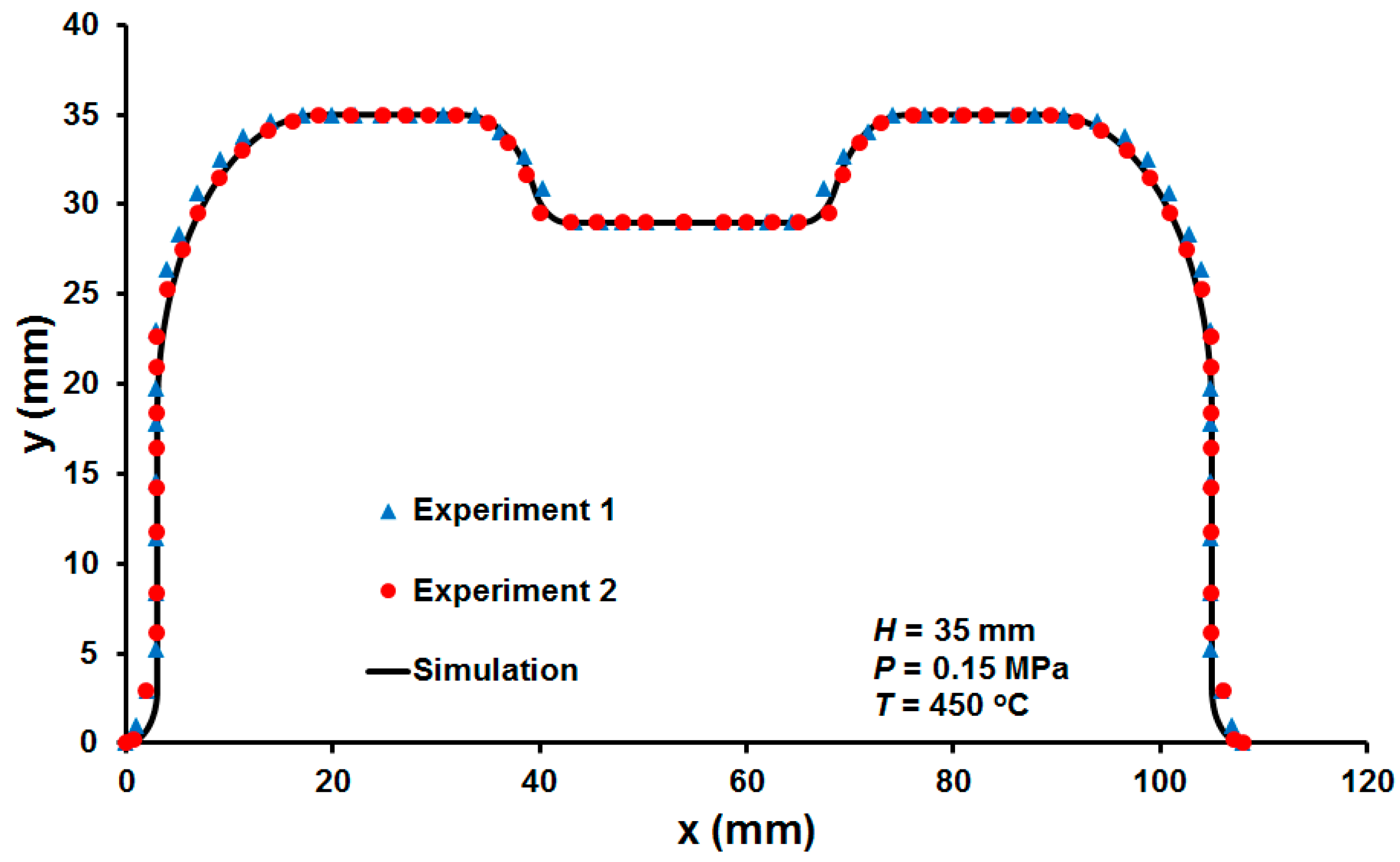
A comparison between the part shape predicted by the simulation and the experimentally measured shape is shown in Figure 15, Figure 16 and Figure 17 for forming using a pressure of 0.15 MPa considering the cup height (H) values of 25, 30, and 35 mm, respectively. The results demonstrate excellent agreement between the experimental and the simulation results for the three considered cases. However, the results of one of the forming experiments, indicated by the blue triangles in Figure 16, differ from those predicted by simulation at the die bottom radius. This occurs at the last stage of the forming process and can be attributed to variations in the material properties of the sheet. When the experiments were repeated, as indicated by the red circle in the same figure, matching results were obtained.

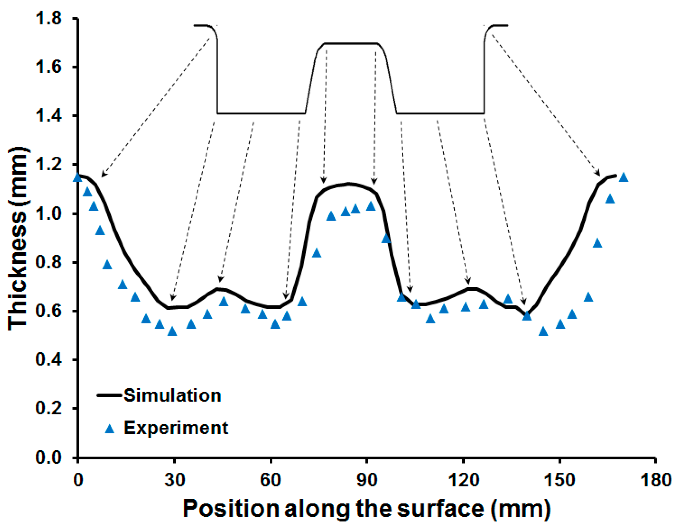
The predicted thickness distribution as a function of the distance along the surface of the formed part using a pressure of 0.15 MPa is shown in Figure 18, Figure 19 and Figure 20 with a cup height of H = 25, 30, and 35 mm, respectively. The results show a good prediction of the cup thickness distribution for the three considered cup heights.

In Figure 18, Figure 19 and Figure 20, arrows were drawn pointing at the regions corresponding to the cup entry radius, cup bottom radius and the boss entry radius. From the experimental results, abrupt changes in the thickness distribution are obvious around the cup entry radius and the boss entry radius. This effect was clearly predicted by the simulation results. The behavior of thinning in the vicinity of the die entry radius has been reported by many researchers [24,31,32,33]. It is attributed to the combined compression and bending effects caused by the small die entry radius, which usually takes place at the beginning of the forming process. However, due to the high value of the coefficient of friction, since no lubricant was used, a near-sticking condition will develop once the sheet gets in contact with the die. Therefore, less material will flow towards the remaining regions of the sheet and more stretching will develop there. Consequently, localized thinning will occur at the die bottom corner, since that region of the sheet is the last to get in contact with the die surface before the forming process ends. This phenomenon was also demonstrated in both the experimental and simulation results in Figure 18, Figure 19 and Figure 20.

3.2. SPF of a Cup with a Car-Shaped Boss

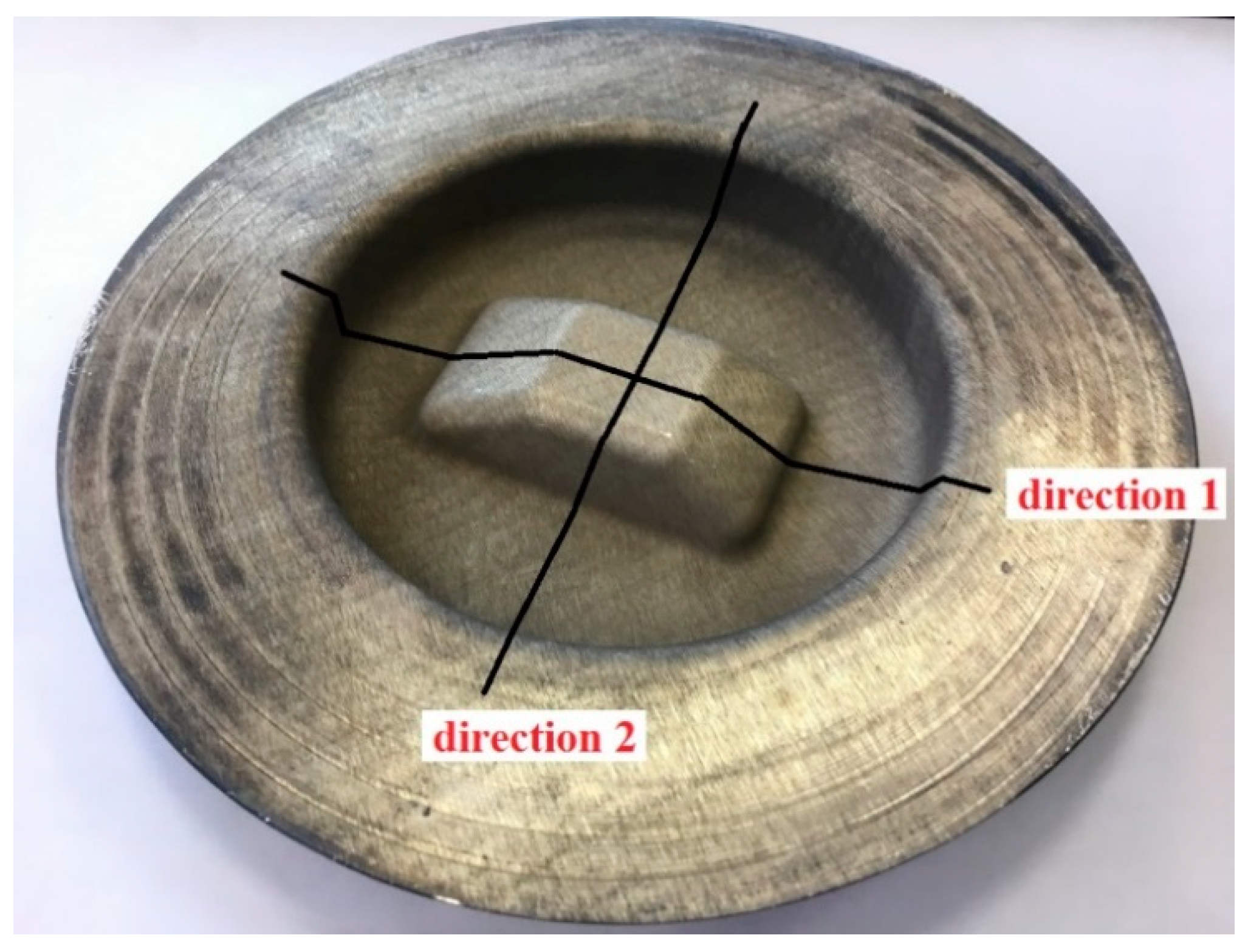
Another complicated geometry was considered for the verification of the constitutive material model. It consisted of a cup with a car-shaped boss. The actual formed part is shown in Figure 21. The forming time was 46.7 min, and the temperature was kept at 450 °C. The part profile and the thickness along two directions (direction 1 and direction 2) were measured for each experiment.

A three-dimensional model in ABAQUS was used to simulate the SPF of the cup with a car-shaped boss. The circular sheet was meshed using 2500 linear quadrilateral shell elements. The die, on the other hand, was modeled using three-dimensional rigid elements.

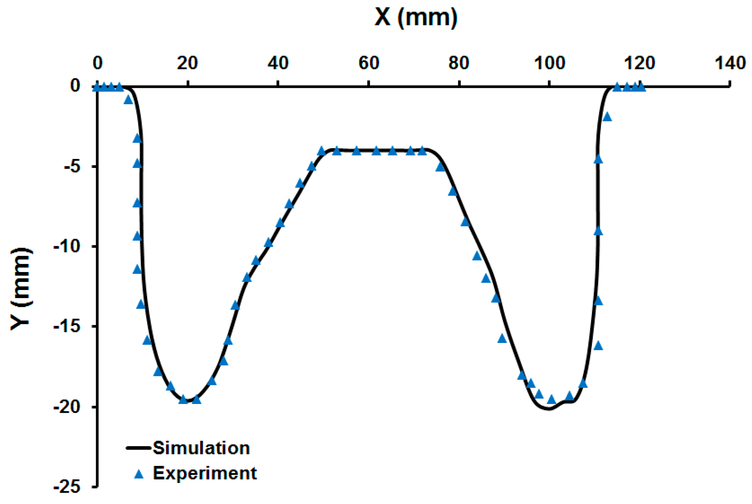
A comparison between the part shape predicted by the simulation and the experimentally measured shape is shown in Figure 22 and Figure 23 for forming using a pressure of 0.3 MPa considering a cup height (H) value of 20 mm. The results demonstrate an excellent agreement between the experimental and the simulation results.

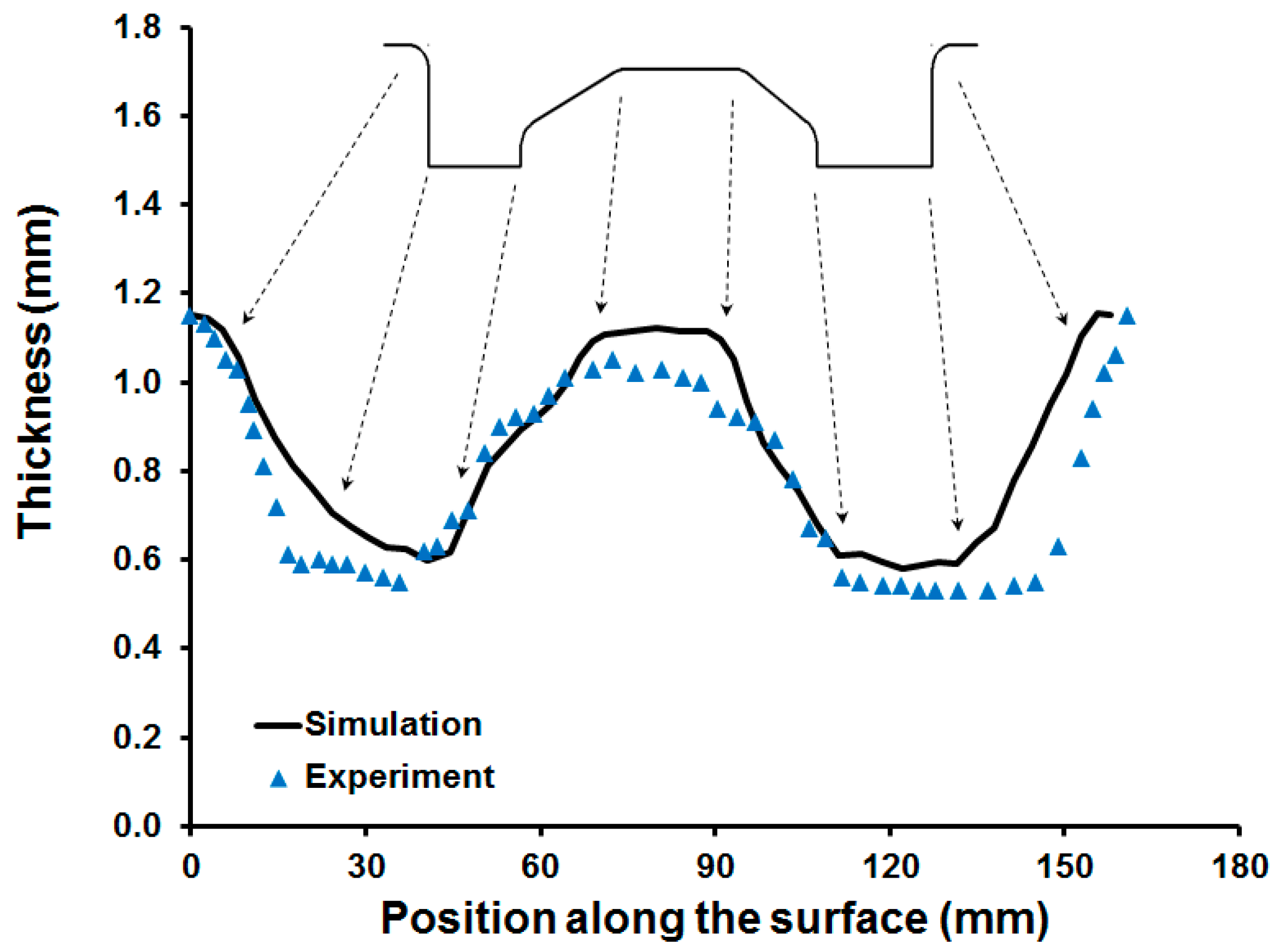
The predicted thickness distribution of the formed car-shape part is shown in Figure 24 and Figure 25. It is interesting to see that the thickness profile and the geometry of the cross-section along each direction show some resemblance. This is expected, since, at the higher parts of the geometry, the sheet will get in contact with the die surface early during the forming process before any considerable stretching occurs. Due to the high coefficient of friction, once in contact no more material flow will happen there, and therefore, the thickness will be relatively higher. Exactly the opposite can be said about the lower parts of the geometry, as they are the last to be in contact with the sheet, a low value of sheet thickness will take place at those regions.

Most of the region along the formed part surface displays a good correspondence between the predicted results and the experimental ones. However, there is a noticeable gap at the bottom radius for direction 1. The prediction of the thickness distribution for direction 2 is slightly better, with only a small difference between the simulation and experimental results at the top of the car-shape profile.

4. Conclusions

The nonlinearities incorporated in the superplastic forming process alongside with the complexity in the material behavior, makes constitutive modeling of such materials a hard challenge. In this study, a constitutive model for AZ31B was established based on a comprehensive numerical-experimental approach. The model takes into account grain growth and cavity formation. The model was calibrated by fitting to data from free bulge forming and microstructure analysis. The fitting process was based on analytical and optimization techniques. Taguchi method was applied in the optimization process. This procedure can be implemented in constitutive modeling of other superplastic materials.

In order to verify the established model, two relatively complicated geometries were simulated, and the results were compared with those obtained from actual SPF experiments. Results show that the material model is capable of predicting the thickness distribution and the shape of the formed part accurately. In fact, the close accord between the experimentally obtained results and the simulation predictions demonstrate the significance of including the microstructure evolution in the AZ31B material model. It is needless to say: This model can be easily implemented in the simulation of the production of complex parts, usually through a material subroutine.

References

- Nieh, T.G.; Wadsworth, J.; Sherby, O.D. Superplasticity in Metals and Ceramics; Cambridge University Press: Cambridge, UK, 1997. [Google Scholar]
- Wadsworth, J.; Sherby, O.D. On the Bulat–Damascus Steels Revisited. Prog. Mater. Sci. 1980, 25, 35–68. [Google Scholar] [CrossRef]
- Kum, D.W.; Oyama, T.; Sherby, O.D.; Ruano, O.A.; Wadsworth, J. Ultrahigh Carbon Steels. JOM 1985, 37, 50–56. [Google Scholar]
- Duygulu, O.; Ozturk, F.; Ucuncuoglu, S.; Secgin, G.O.; Yenice, M.; Kaya, M. Warm Forming of Twin Roll Casted AZ31 Sheet for an Automotive Part. In Proceedings of the 9th International Conference on Magnesium Alloys and their Applications, Vancouver, Canada, 8–12 July 2012; Poole, W.J., Kainer, K.U., Eds.; ResearchGate: Berlin, Germany; pp. 8–12. [Google Scholar]
- Toros, S.; Ozturk, F.; Kaya, M. Modeling Uniaxial, Temperature, and Strain Rate Dependent Behavior of AZ31 Alloy by Softening Model. Key Eng. Mater. 2011, 473, 624–630. [Google Scholar]
- Taleff, E.M.; Hector, L.G., Jr.; Verma, R.; Krajewski, P.E.; Chang, J. Material Models for Simulation of Superplastic Mg Alloy Sheet Forming. J. Mater. Eng. Perform. 2010, 19, 488–494. [Google Scholar] [CrossRef]
- Kappes, J.; Liewald, M. Evaluation of Pneumatic Bulge Test Experiments and Corresponding Numerical Forming Simulations. J. Mater. Sci. Eng. B 2011, 1, 472–478. [Google Scholar] [CrossRef]
- Jarrar, F.; Liewald, M.; Schmid, P.; Fortanier, A. Superplastic forming of triangular channels with sharp radii. J. Mater. Eng. Perform. 2014, 23, 1313–1320. [Google Scholar] [CrossRef]
- Jarrar, F.; Jafar, R.; Tulupova, O.; Enikeev, F.; Al-Huniti, N. Constitutive modeling for the simulation of the superplastic forming of AA5083. Mater. Sci. Forum 2016, 838, 512–517. [Google Scholar] [CrossRef]
- Krajewski, P.E.; Montgomery, G.P. Mechanical Behavior and Modeling of AA5083 at 450 C. In Proceedings of the Advances in Superplasticity and Superplastic Forming, Charlotte, NC, USA, 14–18 March 2004; Taleff, E.M., Friedman, P.A., Krajewski, P.E., Mishra, R.S., Schroth, J.G., Eds.; The Minerals, Metals & Materials Society (TMS): Warrendale, PA, USA, 2004; pp. 341–350. [Google Scholar]
- Jarrar, F.; Sorgente, D.; Aksenov, S.; Enikeev, F. On the Challenges and Prospects of the Superplastic Forming Process. Mater. Sci. Forum 2018, 941, 2343–2348. [Google Scholar] [CrossRef]
- Sorgente, D.; Palumbo, G.; Scintilla, L.; Tricarico, L. Gas forming of an AZ31 magnesium alloy at elevated strain rates. Int. J. Adv. Manuf. Tech. 2016, 83, 861–872. [Google Scholar] [CrossRef]
- Kaya, A.; Eren, D.; Turan, D.; Sorgente, D.; Palumbo, G. Evolution of Microstructure and Texture in AZ31 Alloy Subjected to Gas Forming. JOM 2017, 69, 1041–1045. [Google Scholar] [CrossRef]
- ASTM. Standard Test Methods for Bulge-Forming Superplastic Metallic Sheet; E2717-15; ASTM International: Hawken, PA, USA, 2015. [Google Scholar]
- Franchitti, S.; Giuliano, G.; Palumbo, G.; Sorgente, D.; Tricarico, L. On the optimisation of superplastic free forming test of an AZ31 magnesium alloy sheet. Int. J. Mater. Form. 2008, 1, 1067–1070. [Google Scholar] [CrossRef]
- Nazzal, M.A.; Khraisheh, M.K. Finite Element Modeling of Superplastic Forming in the Presence of Back Pressure. Mater. Sci. Forum 2007, 551–552, 257–262. [Google Scholar] [CrossRef]
- Aksenov, S.A.; Chumachenko, E.N.; Kolesnikov, A.V.; Osipov, S.A. Determination of optimal gas forming conditions from free bulging tests at constant pressure. J. Mater. Process. Technol. 2015, 217, 158–164. [Google Scholar] [CrossRef]
- Jarrar, F.S.; Nazzal, M.A. Inclination angle effect on the thickness distribution in a superplastic formed long rectangular pan. Mater. Sci. Forum 2013, 735, 155–161. [Google Scholar] [CrossRef]
- Jarrar, F. Designing gas pressure profiles for AA5083 superplastic forming. Procedia Eng. 2014, 81, 1084–1089. [Google Scholar] [CrossRef]
- Aksenov, S.A.; Zakhariev, I.Y.; Kolesnikov, A.V.; Osipov, S.A. Characterization of Superplastic Materials by Results of Free Bulging Tests. Mater. Sci. Forum 2016, 838–839, 552–556. [Google Scholar] [CrossRef]
- Dai, G.; Jarrar, F.; Ozturk, F.; Sheikh-Ahmad, J. On the effect of the complexity of the constitutive model in simulating superplastic forming. Defect Diffus. Forum 2018, 385, 379–384. [Google Scholar] [CrossRef]
- Enikeev, F.; Kruglov, A. An analysis of the superplastic forming of a thin circular diaphragm. Int. J. Mech. Sci. 1995, 37, 473–483. [Google Scholar] [CrossRef]
- Caceres, C.; Wilkinson, D. Large strain behaviour of a superplastic copper alloy—I. Deformation. Acta Metall. 1984, 32, 415–422. [Google Scholar] [CrossRef]
- Albakri, M.; Jarrar, F.; Khraisheh, M. Effects of Interfacial Friction Distribution on the Superplastic Forming of AA5083. J. Eng. Mater. Technol. 2011, 133, 031008–031014. [Google Scholar] [CrossRef]
- Jarrar, F.S.; Abu-Farha, F.K.; Hector Jr., L.G.; Khraisheh, M.K. Simulation of High-Temperature AA5083 Bulge Forming with a Hardening/Softening Material Model. J. Mater. Eng. Perform. 2008, 18, 863–870. [Google Scholar] [CrossRef]
- Jarrar, F.S.; Hector Jr, L.G.; Khraisheh, M.K.; Deshpande, K. Gas Pressure Profile Prediction from Variable Strain Rate Deformation Paths in AA5083 Bulge Forming. J. Mater. Eng. Perform. 2012, 21, 2263–2273. [Google Scholar] [CrossRef]
- Li, Z.; Dai, G.; Shi, J.; Jarrar, F.; Ozturk, F.; Sheikh-Ahmad, J. Using the particle swarm optimization method for the constitutive modeling of AZ31B. MSET 2017, 48, 993–997. [Google Scholar] [CrossRef]
- Zhu, J.; Chew, D.; Lv, S.; Wu, W. Optimization method for building envelope design to minimize carbon emissions of building operational energy consumption using orthogonal experimental design (OED). Habitat Int. 2013, 37, 148–154. [Google Scholar] [CrossRef]
- Niu, B.; Liang, J.; Lu, Q.; Chu, X. An orthogonal-design hybrid particle swarm optimiser with application to capacitated facility location problem. IJBIC 2016, 8, 268. [Google Scholar] [CrossRef]
- Chang, T.; Zhan, L.; Tan, W.; Li, S. Optimization of curing process for polymer-matrix composites based on orthogonal experimental method. Fibers Polym. 2017, 18, 148–154. [Google Scholar] [CrossRef]
- Ghosh, A.K.; Hamilton, C.H. Superplastic forming of a long rectangular box section--analysis and experiment. Mater. Process. Congr. 1980, 1978–1979, 303–331. [Google Scholar]
- Harrison, N.R.; Luckey, S.G.; Friedman, P.A.; Xia, Z.C. Influence of Friction and Die Geometry on Simulation of Superplastic Forming of Al-Mg Alloys. In Advances in Superplasticity and Superplastic Forming; The Minerals, Metals & Materials Society (TMS): Warrendale, PA, USA, 2004; pp. 301–309. [Google Scholar]
- Jarrar, F.S.; Hector, L.G., Jr.; Khraisheh, M.K.; Bower, A.F. New approach to gas pressure profile prediction for high temperature AA5083 sheet forming. J. Mater. Process. Technol. 2010, 210, 825–834. [Google Scholar]
Figure 1.
Comparison between uniaxial AZ31B specimens tested at various temperatures.
Figure 2.
Schematic of the gas pressure control system.
Figure 3.
The components of the gas pressure control system used in the experimental SPF setup.
Figure 4.
A ruptured AZ31B circular sheet specimen after high temperature bulge forming.
Figure 5.
The relationship between the grain size at the pole and strain from bulge forming samples under different pressures.
Figure 6.
A schematic diagram of the free bulge forming process.
Figure 7.
Workflow of optimization of parameters A, and ψ.
Figure 8.
Influence of () on the mean square error (MSE) of the pole thickness and dome height at P = 0.15 MPa.
Figure 9.
Influence of () on the MSE of the pole thickness and dome height for P = 0.15 MPa.
Figure 10.
Figure 11.
Influence of () on the MSE of pole thickness and dome height for P = 0.15 MPa.
Figure 12.
A three-dimensional representation of a part consisting of a cup with a cylindrical boss at its base.
Figure 13.
Finished part after 40 min of SPF using a constant gas pressure of 0.15 MPa.
Figure 14.
Axisymmetric model for the SPF of a cup with a cylindrical boss.
Figure 15.
Comparison of the formed shape between experimental and simulation predicted results (H = 25 mm).
Figure 16.
Comparison of the formed shape between experimental and simulation predicted results (H = 30 mm).
Figure 17.
Comparison of the formed shape between experimental and simulation predicted results (H = 35 mm).
Figure 18.
Comparison of the formed part thickness between experimental and simulation predicted results along the specimen surface (H = 25 mm).
Figure 19.
Comparison of the formed part thickness between experimental and simulation predicted results along the specimen surface (H = 30 mm).
Figure 20.
Comparison of the formed part thickness between experimental and simulation predicted results along the specimen surface (H = 35 mm).
Figure 21.
Formed cup with a car-shaped boss.
Figure 22.
Comparison of the formed shape between experimental and simulation predicted results at P = 0.3 MPa (along direction 1).
Figure 23.
Comparison of the formed shape between experimental and simulation predicted results at P = 0.3 MPa (along direction 2).
Figure 24.
Comparison of the formed part thickness between experimental and simulation predicted results along the specimen surface at P = 0.3 MPa (along direction 1).
Figure 25.
Comparison of the formed part thickness between experimental and simulation predicted results along the specimen surface at P = 0.3 MPa (along direction 2).