Abstract
Selective Laser Melting (SLM) is a popular additive manufacturing (AM) method where a laser beam selectively melts powder layer by layer based on the building geometry. The melt pool peak temperature during build process is an important parameter to determine build quality of a fabricated component by SLM process. The melt pool temperature depends on process parameters including laser power, scanning speed, and hatch space as well as the properties of the build material. In this paper, the sensitivity of melt pool peak temperature during the build process to temperature dependent material properties including density, specific heat, and thermal conductivity are investigated for a range of laser powers and laser scanning speeds. It is observed that the melt pool temperature is most sensitive to melt pool thermal conductivity of the processed material for a set of specific process parameters (e.g., laser power and scan speed). Variations in the other mechanical–physical properties of powder and melt pool such as density and specific heat are found to have minimal effect on melt pool temperature.
1. Introduction
Additive manufacturing (AM) is a layer-by-layer manufacturing process that is termed as the next industrial revolution. AM technology has the potential to accelerate innovation, compress supply chains, minimize materials and energy usage, and reduce waste. The most significant benefit of AM technology is its design freedom to address design complexity with no required additional tooling or assembly. In this technology, 3D structures are fabricated layer upon layer by slicing the CAD model. Selective Laser Melting (SLM) is an additive manufacturing technique widely used to fabricate complex 3D components. SLM has been used successfully in different applications including biomedical, aerospace, automotive, and jewelry industries [1,2,3,4,5]. In this process, a laser is scanned over a powder layer and after building one layer, the build plate is lowered by a distance equal to the thickness of the fused layer, and this process of building layers is repeated until fabrication of the whole component is completed [6]. Figure 1 shows a schematic diagram of the SLM process where the main components are a powder bed or base plate, a powder delivery system, an enclosed chamber for operation in a vacuum or an inert gas, and a laser system [7]. The chamber or the build plate can be preheated if necessary.
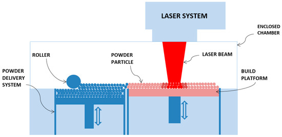
Figure 1.
Schematic of Selective Laser Melting (SLM) system.
Figure 2 shows the major energy transport mechanisms: conduction, convection, and radiation that results in transient heat distribution in the processed zone. Melt pool dynamics is also influenced by the interaction between the laser and liquid metal during solidification process. The spatial and temporal distribution of temperature within and around the melt pool affects microstructure and process induced residual stress in the final product. The finite element analysis (FEA) approach is used by many researchers to model the SLM process, thereby developing process maps and predicting microstructure and residual stress [8,9]. However, there are many difficulties to accurately capture all the features of the SLM process by finite element modeling. Shi et al. [10] mentioned about a splash of powder particle in laser beam track. King et al. [11] discussed strong dynamics of the melted material flow propelled by Marangoni convection during laser melting. Fu et al. [12] performed comparative analysis of melt pool geometry for SLM of Ti-64 alloy and have found a significant difference between FEA and experimental results. In their work, multiple factors such as the accuracy of the thermal input, temperature-dependent properties of both powder and bulk Ti-64, and laser–material interactions were considered to model the SLM process. Yadroitsev et al. [3] investigated experimentally measured melt pool dimensions with theoretical calculations at different irradiation time and found a significant difference between these methods. Verhaeghe et al. [13] created a model for SLM of Ti-64 alloy by considering shrinkage and laser light penetration effects, and studied the influence of incorporating or neglecting evaporation effect in SLM process. Results were not consistent enough to make a conclusion from this study.
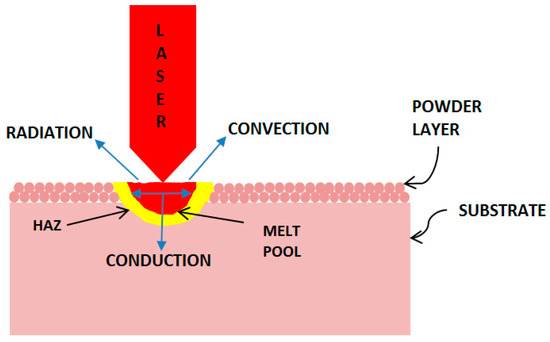
Figure 2.
Schematic of energy transport mechanisms in the laser processed zone.
Since the SLM is a thermal process, the FEA predicted melt pool temperature and geometry heavily depend on the thermal-mechanical properties of metal powders and melt pool liquid metal. It is thus important to understand the sensitivity of FEA predicted melt pool temperatures to thermal–mechanical–physical properties of SLM materials that can help in filling the gap between experimental and simulation results. This analysis will also be useful in any laser melting process where phase change phenomena (e.g., laser welding process) such as solid–liquid–solid occurs [14,15,16,17]. In this paper, sensitivity analysis is performed by creating a finite element model in ABAQUS and by monitoring the melt pool peak temperature by perturbing the properties of Ti-6Al-4V such as specific heat, density, and thermal conductivity. The FEA result is first compared with the experimentally measured temperature using an infrared (IR) camera to understand whether the FEM scheme captures the right trend of the melt pool temperature. Then, each material property is perturbed within the FEM code for several combinations of process parameters such as laser power and laser scanning speed and change in peak temperature is recorded. Only high and low laser powers of 400 W and 91 W, and laser scanning speeds of 1100 mm/s and 200 mm/s are considered in this case. At the end, recommendations on which material property/properties have the most significant effect on melt pool peak temperature during SLM build process are provided.
2. Finite Element Modeling
Finite element modeling technique is being used by many researchers [7,18,19,20,21] for process modeling of selective laser melting (SLM). In SLM process, a moving continuous wave (cw) fiber laser beam with Gaussian type intensity distribution strikes the titanium alloy surface. The heat flow problem can be solved by considering a moving heat source. A description of FEA technique used in this study is presented in following sections.
2.1. Governing Equations
The spatial and temporal temperature distribution T(x,y,z,t) satisfies the following differential equation for three-dimensional heat conduction in a domain D [12,21,22]:
where,
- (x,y,z) = coordinate system attached to the heat source
- Q = power generation per unit volume in the domain D (W m−3)
- kx, ky, kz = thermal conductivity in the x, y and z directions (W m−1 K−1)
- c = specific heat capacity (J kg−1 K−1)
- ρ = density (kg m−3)
- t = time (s)
- v = velocity of laser (m s−1)
The initial condition is,
T(x,y,z,0) = To for (x,y,z) ∈ D
The natural boundary condition can be defined by,
on the boundary, S for (x,y,z) ∈ S and t > 0. S represents those surfaces that are subject to radiation, convection, and imposed heat fluxes. A special case of the imposed heat flux is the adiabatic condition, which represents insulated or symmetry surfaces. Other symbols are defined as:
- kn = thermal conductivity normal to S (W/m-K)
- h = heat transfer coefficient for convection (W/m2-K)
- σ = Stefan–Boltzmann constant for radiation (5.67 × 10⁻⁸ W/m2-K4)
- ε = emissivity
- To = ambient temperature (K)
- q = heat flux normal to S (W/m2)
The inclusion of temperature-dependent thermophysical properties and a radiation term in the above boundary condition makes this type of analysis highly nonlinear.
2.2. Description of the Model
Figure 3 shows the FEA model for the metallic powder layer and the substrate developed in ABAQUS/CAE 2017 (DS Simulia, Providence, RI, USA) [23]. For this model, the substrate is considered to be made of the same material as the powder layer. Model size was determined based on process parameters such as laser beam diameter and scan speed, and mesh convergence is performed to find appropriate mesh size for this analysis. In this model, the size of the substrate is 800 μm × 800 μm × 500 μm and metallic powder layer thickness is 100 μm. The powder bed element size is 20 μm × 20 μm × 20 μm in all directions (x, y, and z). In this particular analysis, powder bed is more important than the substrate; therefore, substrate element size is considered coarser in y-direction with a thickness of 100 μm to save computation time.
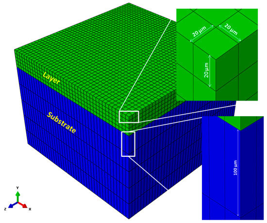
Figure 3.
Single layer of Ti-64 on top of a substrate. In this particular case, the substrate material is also Ti-64. Element sizes in layer and substrate are shown by zooming associated elements.
The moving laser was modeled as a distributed heat flux on the material surface on which the laser is being focused (which is powder surface in this case). Laser irradiation normally has a Gaussian distribution. However, in this case, an average heat flux was calculated by using the following equation and applied in the model [24].
where, α = Absorption coefficient = 0.65 [25], P = laser power in watts, and r0 = radius of laser spot = 50 μm. The moving heat source was modeled by reassigning the location of the distributed heat flux calculated using Equation (4) at different time steps. For example, several element sets, each having laser spot dimension, are chosen on the powder surface. The distributed heat flux was applied on the element set 1 in load step 1 and nodal temperatures are numerically calculated utilizing Equation (1). Heat flux was then applied on the element set 2 in the second load step, and so on. Thus, a nodal temperature history was obtained as a function of time. The time was calculated based on the scanning velocity and heat source location. The transient heat transfer model was then run and nodal temperature was documented as a function of time for use in the subsequent steps.
Both convection and radiation boundary conditions were applied in this model. Initial and boundary conditions are tabulated in Table 1. Convective heat transfer coefficient was considered as 20 W/m2-K that is the average value for air [26] and radiation emissivity was considered to be 0.35 [17].

Table 1.
Initial and boundary conditions.
2.3. Material Properties
Material properties are the essential input parameters for the model. For different materials, associated material properties can be used to find temperature distribution within the model. Three material properties—density, specific heat, and thermal conductivity—were varied within the model to understand their influence on melt pool peak temperature. The temperature dependent base properties used for the reference model are shown in Equations (5)–(7) for a temperature range of 273 K to 3023 K for Ti64 alloy. Equations (5)–(7) were generated from a linear fit of the data published in references [17,27,28]. One of the reasons for choosing linear fit is that it will facilitate further analysis of the sensitivity of peak temperature to variation in these properties that are described in the later section of this paper.
2.4. Experimental Data to Verify Reference FEA Model
The model response in this analysis is considered to be the melt pool peak temperature during the build process. The finite element model developed was first run for the base material properties listed in Equations (5)–(7) and temperature contour plot was recorded (Figure 4) for a process parameter set of 91 W and 200 mm/s. The FEA predicted melt pool temperature was observed to be high; however, a similar order of peak temperature also reported by Fu et al. [13]. The numerically calculated melt pool temperature was then compared with experimental measurements.
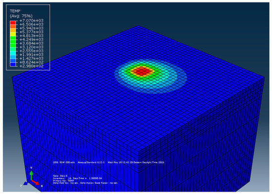
Figure 4.
Surface temperature distribution at a laser power of 91 W with scanning speed, 200 mm/s.
An in-house-built SLM machine was utilized for the experiments to create a single bead Ti-64 sample. This SLM machine is equipped with a cw Yb fiber laser, which produces a laser beam with a wavelength of 1064 mm and a maximum of 500 W power. A focused laser beam is guided through an optical system to the desired positions of the powder bed to melt the Ti-6Al-4V metallic powder. In this case, the powder particles are mostly spherical in shape with the average particle size of 40 µm. Ti-6Al-4V is an alloy that consists of an alpha-beta phase. Chemical composition of the powder is shown in Table 2 [29]. The bed is not preheated, and room temperature is maintained inside the chamber. Argon gas atmosphere is created inside the closed chamber. Single scans are performed for a matrix of laser power and scan speed. The laser beam diameter and layer thickness are maintained as constant throughout the experiments.
Table 2.
Chemical composition of Ti-6Al-4V.
An infrared (IR) camera, model XEVA-FPA-1.7-320 (Xenics Infrared Solutions, BE-3001 Leuven, Belgium), is used to measure real-time temperature during SLM build process. Maximum temperature is identified from the dark red zone of IR images for each bead. The maximum numerical value for each bead is considered as peak temperature. The pixel size of the IR camera is 1 mm × 1 mm. It can be noted that due to the larger pixel size of the camera, peak temperature value from IR camera is smaller than the actual value. After averaging finite element data to camera pixel size, peak temperature data from IR camera and FEM results are compared in Figure 5. It was observed that the temperature values are quite comparable, and the difference is around 131–159 °C.
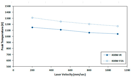
Figure 5.
Comparison of maximum FEA temperature that is averaged over a camera pixel and IR data of Ti-64 sample at 400 W and 200 to 1100 mm/s.
The melt pool width of the fabricated single bead was measured using a confocal microscope by viewing from top of the sample. The width measurements were done along the length of the sample and were averaged for a particular process parameter. Representative confocal microscopy images of single beads created with laser power of 400 W at scanning speed of 200 mm/s are shown in Figure 6a,b. The melt pool width was also obtained from the FEA model by monitoring the melt pool whose temperature was above the melting point of 1300 C. The measured width is compared with the FEA predictions and is shown in Figure 7. It was observed that the difference is around 44–124 μm between experimental and FEA values. It has been discussed previously in the introduction section by referencing other research work [12] where finite element results are seen to deviate from experimental data in the same order of magnitude. It is one of the objectives of this sensitivity study to work towards a solution to minimize the difference. In particular, the sensitivity of FEA predicted melt pool peak temperature to material properties is investigated in detail.
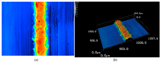
Figure 6.
(a) Two-dimensional and (b) three-dimensional confocal microscopy images of single beads Ti-64 samples produced at laser power of 400 W at scanning speed of 200 mm/s.

Figure 7.
Melt-pool width of Ti-64 beads at 400 W laser power and 200–1100 mm/s sweeping speed.
3. Variation in Material Properties
Once the melt pool temperature was calculated for the base model, various materials properties of the model are varied to find their influence on the melt pool temperature. One of the ways of changing material properties is by changing the slope of the material property vs. temperature plots. The material properties that were used to generate a wide range of melt pool temperatures as a function of material properties are shown in Figure 8, Figure 9, Figure 10, Figure 11 and Figure 12. Figure 8 shows the temperature vs. density plots where the slope of the base density plot is considered as −0.23 kg/m3/K (also presented by Equation (5)). The slope is varied from −0.15 to −0.3 kg/m3/K to generate five sets of density data. Similarly, the slope of the base specific heat plot is 0.2 J/kg-K/K and is varied between 0.1 J/kg-K/K and 0.3 J/kg-K/K to generate five sets of specific heat data (Figure 9). The temperature dependent thermal conductivity used for the analysis is shown in Figure 10, where the base slope is 0.0139 W/m-K/K and was varied from 0.005 W/m-K/K to 0.03 W/m-K/K to create seven sets of data. In addition, thermal conductivity was varied before and after melting point to identify which one has more significant effect on melt pool temperature. These variations are shown in Figure 11 and Figure 12, where slopes are varied only before and after melting temperature, respectively.

Figure 8.
Density vs temperature plot with varying slopes.
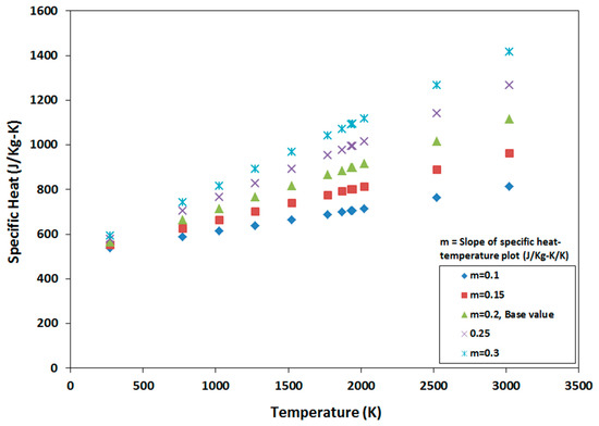
Figure 9.
Sets of specific heat data by varying its slope from the base slope of 0.2 J/kg-K/K.

Figure 10.
Seven sets of thermal conductivity data generated by varying the base slope (shown in Equation (7)) between 0.005 and 0.03 W/m-K/K.

Figure 11.
Slope of thermal conductivity data before melting point is varied.
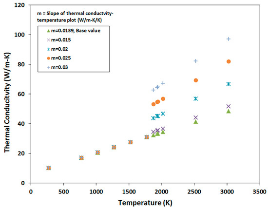
Figure 12.
Slope of thermal conductivity data after the melting point is varied.
4. Results and Discussion
In this section, the influence of density, specific heat, and thermal conductivity on peak melt pool temperature is analyzed for laser powers of 400 W and 91 W, and laser scanning speeds of 200 mm/s and 1100 mm/s.
4.1. Sensitivity to Density
To find the sensitivity of peak temperature to density for a range of laser power and laser scanning speed, simulation was performed by changing density data according to Figure 8 while keeping specific heat and thermal conductivity to its base values as shown in Equations (6) and (7). The percent change of peak temperature with respect to base density for two laser powers 400 W and 91 W and two laser scanning speeds 200 mm/s and 1100 mm/s are plotted in Figure 13. Peak temperature changes due to varying density are up to 1.31%, which is expressively low, and it can be concluded that density does not have a significant effect on peak build temperature.

Figure 13.
Sensitivity of peak temperature to density. Percentage change of peak temperature with respect to that calculated with base density at different process parameters.
4.2. Sensitivity to Specific Heat
In the case of specific heat, five sets of specific heat data (Figure 9) were used in the simulation while base density and thermal conductivity (Equations (5) and (7)) were kept constant. In Figure 14, the minimum and maximum percent change of peak temperature due to varying slope of specific heat are 0% and 7.57%. It can be concluded that the variation in specific heat does not have any significant effect on peak temperature.
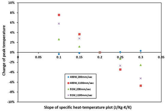
Figure 14.
Sensitivity of peak temperature to specific heat. Percentage change of peak temperature with respect to that calculated with base specific heat at different process parameters.
4.3. Sensitivity to Thermal Conductivity
Applying a similar method as discussed earlier, the percent change of peak temperature was numerically calculated by varying thermal conductivity and is shown in Figure 15. It can be noted that the change in peak temperature with respect to base value is high enough to conclude that the thermal conductivity has a significant effect on peak temperature during SLM build process. The percent change of peak temperature varies up to 48% for the thermal conductivities used in the current simulation.
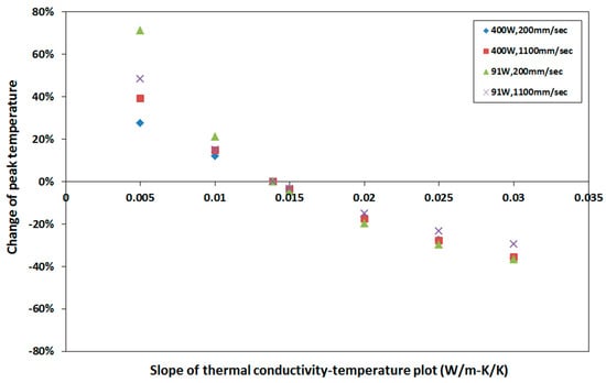
Figure 15.
Sensitivity of peak temperature to thermal conductivity. Percentage change of peak temperature with respect to that calculated with base thermal conductivity at different process parameters.
To further understand the effect of thermal conductivity, it was varied up to melting point only and the percent change in peak temperature was calculated and plotted in Figure 16. It was observed that the maximum change in peak temperature is only 5%. On the other hand, when thermal conductivity is varied after melting point only, the change in peak temperature is up to 36%, which is presented in Figure 17. It is also observed from Figure 17 that higher the melt pool conductivity, the lower is the melt pool peak temperature and vice versa. The results shown in Figure 16 and Figure 17 are intuitively correct as the heat transfer rate is relatively higher at the molten state once the melting process is completed due to melt pool dynamics.

Figure 16.
Sensitivity of peak temperature to thermal conductivity. Change of peak temperature with respect to that calculated with base thermal conductivity at varying process parameters. Slope of thermal conductivity–temperature plot before the melting point is varied only.

Figure 17.
Sensitivity of peak temperature to thermal conductivity. Change of peak temperature with respect to that calculated with base thermal conductivity at varying process parameters. Slope of thermal conductivity–temperature plot after the melting point is varied only.
5. Summary
The sensitivity of melt pool temperature during SLM process to material properties such as density, specific heat, and thermal conductivity are studied for four sets of process parameters. They are: laser powers of 400 W and 91 W, and laser scanning speeds of 200 mm/s and 1100 mm/s. It was observed that perturbation in density and specific heat does not cause any significant change in melt pool peak temperature. On the other hand, thermal conductivity has a significant effect on melt pool peak temperature. More explicitly, thermal conductivity after the melting point has the most substantial effect on peak temperature. Thus, it can be concluded that more care must be taken on melt pool thermal conductivity to more accurately predict the temporal and spatial distribution of temperature in and around the melt pool using FEA. Accurate prediction of temperature distribution is paramount to predicting microstructural and mechanical properties of SLM parts.
Author Contributions
Conceptualization, S.H.A. and A.M.; methodology, S.H.A.; software, S.H.A.; validation, S.H.A.; formal analysis, S.H.A. and A.M.; resources, A.M.; data curation, S.H.A.; writing—original draft preparation, S.H.A.; writing—review and editing, A.M.; visualization, S.H.A.; supervision, A.M.; project administration, A.M.; funding acquisition, A.M.
Funding
This research was funded by Advratech, LLC, grant number 669845.
Acknowledgments
The authors thank Chandrakanth Kusuma and Advratech engineers for experimental tests and insightful discussions.
Conflicts of Interest
The authors declare no conflict of interest.
References
- Nickels, L. 3D printing the world’s first metal bicycle frame. Met. Powder Rep. 2014, 69, 38–40. [Google Scholar] [CrossRef]
- Conner, B.P.; Manogharan, G.P.; Martof, A.N.; Rodomsky, L.M.; Rodomsky, C.M.; Jordan, D.C.; Limperos, J.W. Making sense of 3-D printing: Creating a map of additive manufacturing products and services. Addit. Manuf. 2014, 1–4, 64–76. [Google Scholar] [CrossRef]
- Yadroitsev, I.; Krakhmalev, P.; Yadroitsava, I. Selective laser melting of Ti6Al4V alloy for biomedical applications: Temperature monitoring and microstructural evolution. J. Alloys Compd. 2014, 583, 404–409. [Google Scholar] [CrossRef]
- Bertol, L.S.; Júnior, W.K.; da Silva, F.P.; Aumund-Kopp, C. Medical design: Direct metal laser sintering of Ti–6Al–4V. Mater. Des. 2010, 31, 3982–3988. [Google Scholar] [CrossRef]
- Jewellery and Watches—DMLS for Individual Specimens and Serial Production. EOS. Available online: http://www.eos.info/industries_markets/lifestyle_products/jewellery_watches (accessed on 9 September 2016).
- Galba, M.; Reischle, T. Additive manufacturing of metals using powder-based technology. In Additive Manufacturing; CRC Press: Boca Raton, FL, USA, 2015; pp. 97–142. [Google Scholar]
- Srivatsan, T.S.; Sudarshan, T.S. (Eds.) Additive Manufacturing: Innovations, Advances, and Applications; CRC Press: Boca Raton, FL, USA, 2015. [Google Scholar]
- Bontha, S.; Klingbeil, N.W.; Kobryn, P.A.; Fraser, H.L. Effects of process variables and size-scale on solidification microstructure in beam-based fabrication of bulky 3D structures. Mater. Sci. Eng. A 2009, 513–514, 311–318. [Google Scholar] [CrossRef]
- Bontha, S.; Klingbeil, N.W.; Kobryn, P.A.; Fraser, H.L. Thermal process maps for predicting solidification microstructure in laser fabrication of thin-wall structures. J. Mater. Process. Technol. 2006, 178, 135–142. [Google Scholar] [CrossRef]
- Shi, Q.; Gu, D.; Xia, M.; Cao, S.; Rong, T. Effects of laser processing parameters on thermal behavior and melting/solidification mechanism during selective laser melting of TiC/Inconel 718 composites. Opt. Laser Technol. 2016, 84, 9–22. [Google Scholar] [CrossRef]
- King, W.E.; Anderson, A.T.; Ferencz, R.M.; Hodge, N.E.; Kamath, C.; Khairallah, S.A.; Rubenchik, A.M. Laser powder bed fusion additive manufacturing of metals; physics, computational, and materials challenges. Appl. Phys. Rev. 2015, 2, 041304. [Google Scholar] [CrossRef]
- Fu, C.H.; Guo, Y.B. Three-Dimensional temperature gradient mechanism in selective laser melting of Ti-6Al-4V. J. Manuf. Sci. Eng. 2014, 136, 061004. [Google Scholar] [CrossRef]
- Verhaeghe, F.; Craeghs, T.; Heulens, J.; Pandelaers, L. A pragmatic model for selective laser melting with evaporation. Acta Mater. 2009, 57, 6006–6012. [Google Scholar] [CrossRef]
- Casalino, G.; Mortello, M.; Peyre, P. FEM analysis of fiber laser welding of titanium and aluminum. Procedia CIRP 2016, 41, 992–997. [Google Scholar] [CrossRef]
- Jiang, P.; Wang, C.; Zhou, Q.; Shao, X.; Shu, L.; Li, X. Optimization of laser welding process parameters of stainless steel 316L using FEM, Kriging and NSGA-II. Adv. Eng. Softw. 2016, 99, 147–160. [Google Scholar] [CrossRef]
- Prashanth, K.G.; Damodaram, R.; Scudino, S.; Wang, Z.; Prasad Rao, K.; Eckert, J. Friction welding of Al–12Si parts produced by selective laser melting. Mater. Des. 2014, 57, 632–637. [Google Scholar] [CrossRef]
- Wits, W.W.; Becker, J.M.J. Laser beam welding of titanium additive manufactured parts. Procedia CIRP 2015, 28, 70–75. [Google Scholar] [CrossRef]
- Kolossov, S.; Boillat, E.; Glardon, R.; Fischer, P.; Locher, M. 3D FE simulation for temperature evolution in the selective laser sintering process. Int. J. Mach. Tools Manuf. 2004, 44, 117–123. [Google Scholar] [CrossRef]
- Hussein, A.; Hao, L.; Yan, C.; Everson, R. Finite element simulation of the temperature and stress fields in single layers built without-support in selective laser melting. Mater. Des. 2013, 52, 638–647. [Google Scholar] [CrossRef]
- Dong, L.; Makradi, A.; Ahzi, S.; Remond, Y. Three-dimensional transient finite element analysis of the selective laser sintering process. J. Mater. Process. Technol. 2009, 209, 700–706. [Google Scholar] [CrossRef]
- Mahmood, T.; Mian, A.; Amin, M.; Auner, G.; Witte, R.; Herfurth, H.; Newaz, G. Finite Element Modeling of Transmission Laser Microjoining Process. J. Mater. Process. Technol. 2007, 186, 37–44. [Google Scholar] [CrossRef]
- Carslaw, H.S.; Jaeger, J.C.; Feshbach, H. Conduction of heat in solids. Phys. Today 1962, 15, 74. [Google Scholar] [CrossRef]
- ABAQUS/CAE. 2017. Available online: https://www.3ds.com/products-services/simulia/ (accessed on 16 April 2019).
- Shi, Y.; Shen, H.; Yao, Z.; Hu, J. Temperature gradient mechanism in laser forming of thin plates. Opt. Laser Technol. 2007, 39, 858–863. [Google Scholar] [CrossRef]
- Romano, J.; Ladani, L.; Razmi, J.; Sadowski, M. Temperature distribution and melt geometry in laser and electron-beam melting processes—A comparison among common materials. Addit. Manuf. 2015, 8, 1–11. [Google Scholar] [CrossRef]
- Pope, J.E. Rules of Thumb for Mechanical Engineers: A Manual of Quick, Accurate Solutions to Everyday Mechanical Engineering Problems; Gulf Pub.: Houston, TX, USA, 1997. [Google Scholar]
- Mills, K.C. Recommended Values of Thermophysical Properties for Selected Commercial Alloys; ASM International: Materials Park, OH, USA; Cambridge, UK, 2001. [Google Scholar]
- Boivineau, M.; Cagran, C.; Doytier, D.; Eyraud, V.; Nadal, M.; Wilthan, B.; Pottlacher, G. Thermophysical properties of solid and liquid Ti-6Al-4V (TA6V) alloy. Int. J. Thermophys. 2006, 27, 507–529. [Google Scholar] [CrossRef]
- Kusuma, C.; Ahmed, S.; Mian, A.; Srinivasan, R. Effect of Laser Power and Scan Speed on Melt Pool Characteristics of Commercially Pure Titanium (CP-Ti). J. Mater. Eng. Perform. 2017, 26, 3560–3568. [Google Scholar] [CrossRef]
© 2019 by the authors. Licensee MDPI, Basel, Switzerland. This article is an open access article distributed under the terms and conditions of the Creative Commons Attribution (CC BY) license (http://creativecommons.org/licenses/by/4.0/).