An Evolutionary Yield Function Model Based on Plastic Work and Non-Associated Flow Rule

1
Department of Integrated Systems Engineering, Ohio State University, 210 Baker Systems, 1971 Neil Avenue, Columbus, OH 43210, USA
2
Department of Automotive Engineering, Clemson University, Greenville, SC 29607, USA
*
Author to whom correspondence should be addressed.
Metals 2019, 9(5), 611; https://doi.org/10.3390/met9050611
Submission received: 14 April 2019
/
Revised: 10 May 2019
/
Accepted: 19 May 2019
/
Published: 25 May 2019
(This article belongs to the Special Issue Constitutive Modelling for Metals)
Abstract
:A constitutive law was developed based on the evolutionary yield function to account for the evolution of anisotropy induced by the plastic deformation. For the effective description of anisotropy, the yield stress function and plastic potential were separately defined based on the non-associated flow rule. In particular, for the description of the equivalent status, the accumulated plastic work was employed as an alternative to the accumulated plastic strain. Numerical formulations based on the plastic work were also derived in case the hardening rule, as well as the evolution of the plastic potential and yield stress function, were defined in terms of the plastic work. The developed constitutive law was characterized using the mechanical properties of the multi-phase BAO QP980 steel and niobium sheets at room temperature. From the uniaxial tension tests and the balanced biaxial tension test, separate sets of anisotropic coefficients for each of the plastic potential and yield stress functions were obtained as a function of the plastic work. By comparing with non-evolving yield functions, the importance of the developed constitutive law to properly describe the evolution of the plastic potential and yield function were validated.
1. Introduction
New sheet metal alloys are continuously being developed to meet the mechanical properties required for various industries. In particular, in the automotive industry, the demand for lightweight alloys and advanced high strength steels is gradually increasing, due to these metals’ improved formability and specific strength, which are necessary for better crashworthiness as well as the reduction in the vehicle weight. In response to the introduction of the new metal alloys, advanced constitutive laws have been developed to improve the numerical prediction capability of finite element models for such parameters as formability and spring-back of stamped sheet metals.
In classical plasticity, the constitutive laws mainly consist of the yield stress function to describe the boundary between elastic and elasto-plastic regions, the plastic potential to define the plastic strain increment based on the normality rule, and hardening rules to describe the evolution of the yield function. In particular, for the description of planar anisotropy of sheet materials, various yield functions and their evolution laws have been proposed. Hill [1] proposed a quadratic yield function, while non-quadratic yield functions [2,3,4,5,6,7,8] have been developed over the years based on Karafillis and Boyce [9] type yield function.
In the associated flow rule, the plastic potential is assumed to be identical with the yield stress function. This simple hypothesis has a significance in the numerical analysis and also satisfies the Drucker [10] stability postulate for stable materials. However, as Stoughton [11] pointed out, the fact that fundamental theorems are rigorously proven based on the associated flow rule, does not imply that the associated flow rule is always true. If a precise description of anisotropy is desired, complicated functions with a large number of parameters must be used in the associated flow rule to simultaneously account for the anisotropy of both the yield stress function and the plastic potential. Alternatively, separate functions can be defined to represent the anisotropy of the plastic potential and the yield stress function. Compared with the associated flow rule, less complex functions could be used in the non-associated flow rule to define the plastic potential and the yield stress function [11,12,13,14,15,16,17,18,19]. The constraints to ensure stability in the non-associated flow rule were derived by [13,15]. Also, Spitzig [20] reported violation of the associated flow rule during the plastic deformation under the hydrostatic pressure.
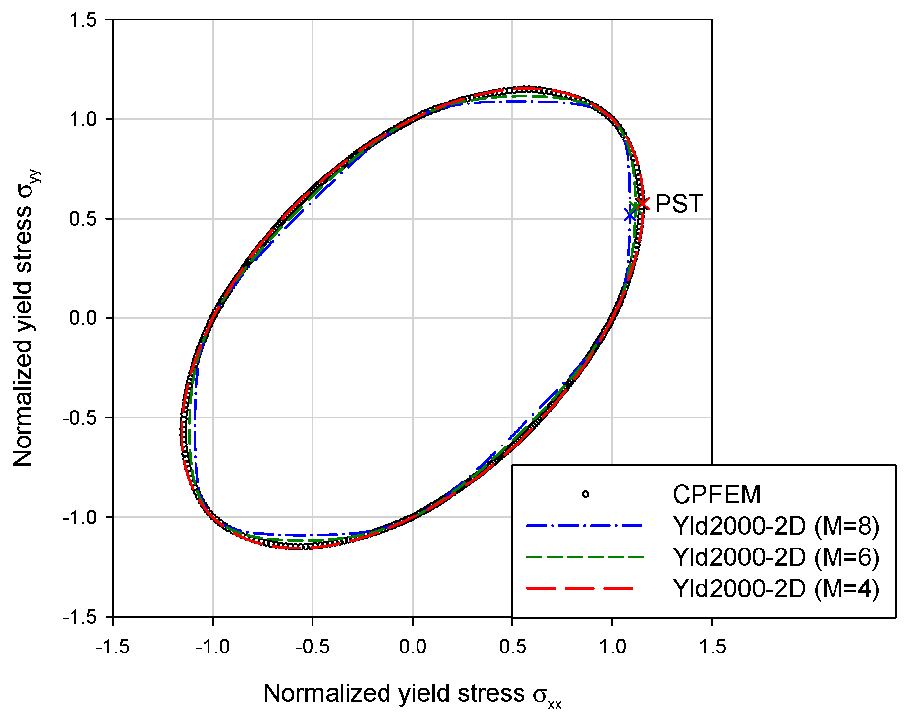
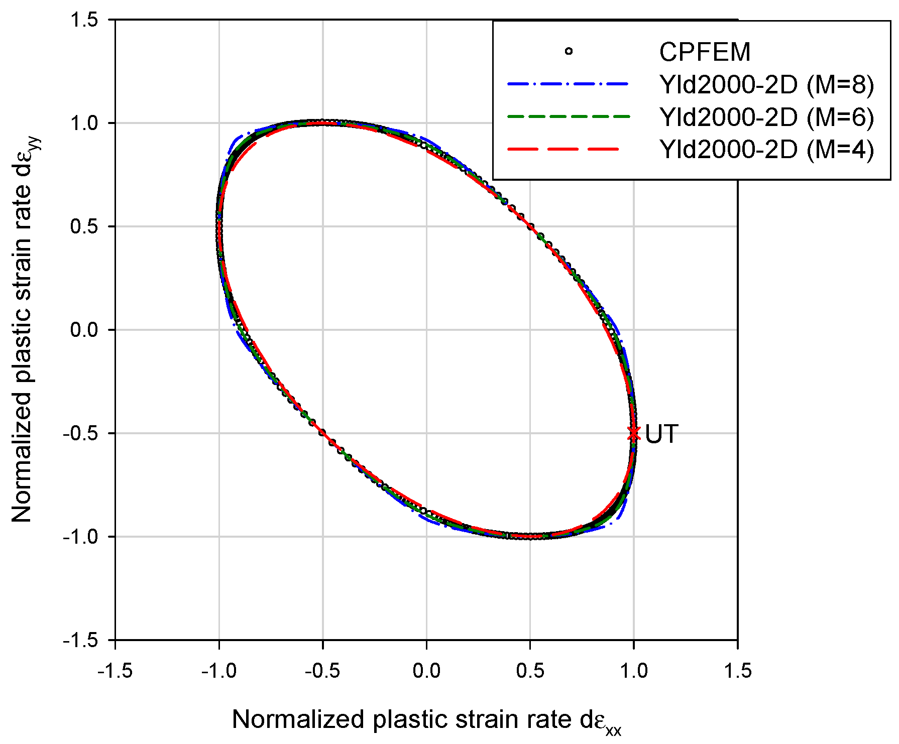
For a demonstration, isotropic yield surfaces and their conjugate strain-rate potentials were generated based on crystal plasticity [21] and Yld2000-2d function [3]. In order to have the initial isotropy in the crystal plasticity simulations, initial crystal orientations were randomly generated and assigned to 8000 grains. Considering face centered cubic (FCC) crystals with 12 slip systems (<110> slip directions on ({111} slip planes), the crystal plasticity simulations were performed for a total of 360 stress ratios between x- and y- directions under the plane stress condition. As for the Yld2000-2d function, all the anisotropy coefficients were set to 1.0 to generate isotropic yield surface and three yield exponents (m = 4, 6, and 8) were considered to generate non-quadratic yield surfaces. As shown in Figure 1, the isotropic yield surface based on the Yld2000-2d function with a yield exponent of 4 is in good agreement with the yield surface generated by the crystal plasticity simulations. However, in the case of the strain-rate potential shown in Figure 2, the prediction based on the Yld2000-2d function with a yield exponent of 6 shows the most similar results to the case of the crystal plasticity simulations. These results imply that, not only it is not necessary but that it is also insufficient, to use the same function to represent the anisotropy of the plastic potential and the yield stress function.
In the meantime, various attempts have been made to account for the anisotropic evolution of the yield surface. Hill and Hutchinson [22] proposed a theoretical framework, which is relevant to the differential hardening of a sheet material subjected to the arbitrary biaxial tensions. Abedrabbo et al. [23,24] used polynomial functions to fit the anisotropic coefficients of Barlat Yld96 anisotropic yield function [2] for different temperatures and strain rates. Plunkett et al. [25] developed an elastic-viscoplastic model to describe the anisotropic/asymmetric evolution of the yield surface as a function of the accumulated plastic strain based on CPB06 yield function [6]. Zamiri and Pourboghrat [26] developed an evolutionary yield function, which describes the evolution of the anisotropic coefficients of Hill’s quadratic yield function [1] during the plastic deformation as a function of the plastic strain. Aretz [27] described the impact of distortional hardening on the prediction of forming limit curves. Stoughton and Yoon [16] also utilized Hill’s model [1] to provide a framework for the non-associated flow rule accounting for the anisotropic hardening in proportional loading. Although the evolution of the yield stress function was defined using a less complicated model and independent of the plastic potential, improved accuracy in the prediction of the uniaxial tension stress–strain curves was observed compared with the associated flow rule models.
Further efforts were made to account for the Bauschinger effect in the non-monotonous loading conditions. Chung and Park [28] proposed a consistency condition for the combined type isotropic-kinematic hardening law, in which the combined type hardening law is expected to behave the same as the full isotropic hardening for monotonously proportional loading. By partially releasing the consistency condition with an introduction of a homogeneous function to control the anisotropic back stress evolution, anisotropic hardening behavior was accurately described preserving the proportionality between global stress and back stress. Yoshida et al. [29] also proposed a material model to consider the anisotropic and nonlinear kinematic hardening as well as the cyclic hardening phenomena with the non-associated flow rule.
In this work, a constitutive law to describe the evolution of anisotropy induced by the plastic deformation was developed based on the evolutionary yield function. For effective description, the yield stress function and the plastic potential as well as their evolutions were separately defined based on the non-associated flow rule. An asymptotic evolution equation was employed for the general description of the separate sets of the anisotropic coefficients for each of the plastic potential and yield stress function. As an alternative to using the accumulated equivalent plastic strain, the authors decided to employ a more general term such as the accumulated plastic work in order to impose the equivalency between various experimental data.
As will be discussed in this paper, the evolution of the yield function and the plastic potential can be explicitly characterized by using the accumulated plastic work. The reason for this is that the plastic work increment can be directly calculated from the plastic strain increment and stress components regardless of the definition of the yield function and the plastic potential. It is important to note that unlike the plastic work increment, the equivalent plastic strain increments are dependent on the definition of the yield function and the plastic potential. This makes it difficult to impose the equivalency between various experimental data especially when the yield stress and plastic potential functions evolve during the plastic deformation.
As a demonstration of the developed evolutionary constitutive law, mechanical properties of BAO Q&P 980 multi-phase steel and niobium sheets at room temperature were characterized for the developed evolutionary model. The experimental data obtained from the uniaxial tension test is summarized in Section 2. The general framework for the development of the constitutive law is described in Section 3. Details of the material characterization methodology for the developed constitutive law are described in Section 4. A comparison of the evolutionary non-associated yield function with non-evolutionary yield function is discussed in Section 5 by performing simulations of uniaxial tension and biaxial cup drawing tests. Section 6 provides the concluding remarks.
2. Experiments
In this work, mechanical properties of BAO Q&P 980 steel and niobium sheets at room temperature were characterized for the developed evolutionary model. Further details on the heat treatment of the Q&P 980 (Fe-0.2C-1.8Mn-1.5Si) steel and the chemical composition of the high purity superconducting niobium sheet can be found in the former publications [26,30,31]. Overall, the Q&P 980 steel shows mild anisotropy, while the niobium sheet exhibits highly anisotropic behavior. These two extreme behaviors were chosen to showcase the importance of applying an evolutionary yield function compared with non-evolving yield functions.
For the Q&P 980 steel, the tensile tests were carried out based on ASTM E8M standard procedures using an Instron universal material testing machine. The tensile grip speed was maintained at 10 mm/min, which corresponds to approximately 0.0024/s in engineering strain rate. In order to measure the anisotropy, specimens were prepared along 0, 15, 30, 45, 60, 75 and 90 degrees off to the rolling direction. The strain histories were measured by an ARAMIS 5M digital image correlation (DIC) system manufactured by GOM GmbH, Braunschweig, Germany.
As for the niobium sheet, tensile tests were performed according to ASTM E517 [32]. The tensile grip speed was set to 0.25 mm/s, which is corresponding to 0.01/s in engineering strain rate considering the 25 mm gauge length. For the anisotropic evolution, the tensile tests were performed along 0, 22.5, 45, 67.5 and 90 degrees off the rolling direction.
For each direction, the tensile tests were repeated 3 and 5 times for the Q&P 980 steel and niobium sheet, respectively, and averaged mechanical properties were obtained. The averaged Young’s moduli (E), 0.2% offset true yield strengths (YS), uniform elongations (UE), engineering ultimate tensile strength (UTS), and total elongations (TE) for the Q&P 980 steel and niobium sheets are summarized in Table 1 and Table 2, respectively.
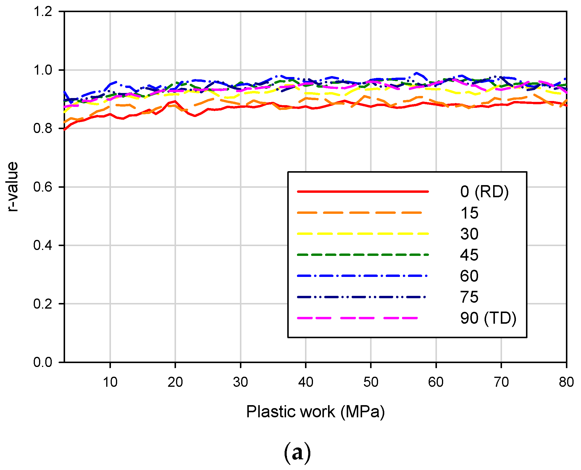
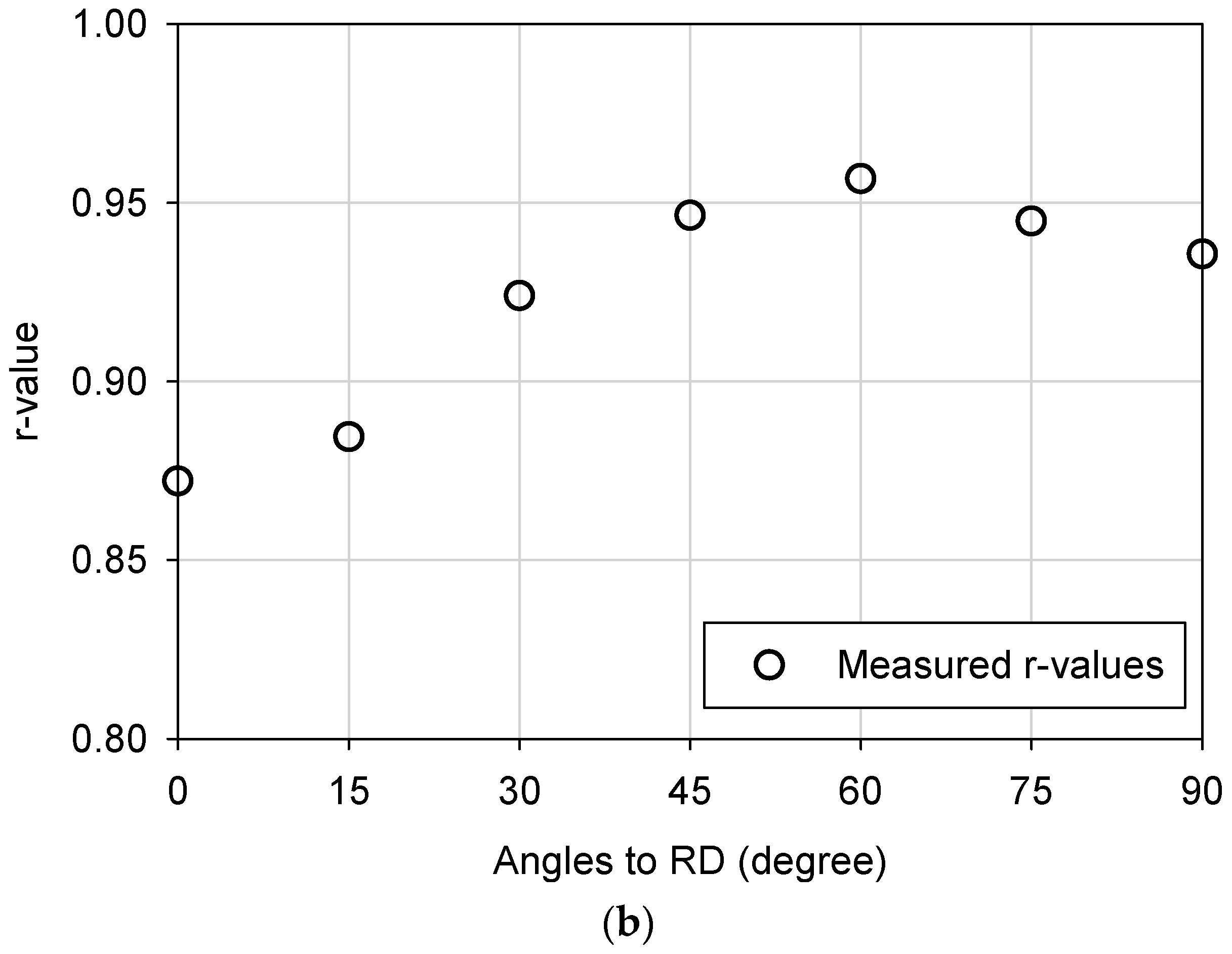
Based on the measured strain histories, r-values (: width-to-thickness plastic strain increment ratio in the uniaxial tensile test) could be calculated by eliminating the elastic strain increments from the measured strain increments. The elastic strain increments were calculated from the stress increments assuming Hooke’s law and the corresponding plastic work increment was calculated from the obtained plastic strain increments.
In this work, instead of the (accumulated) equivalent plastic strain, the accumulated plastic work was used for the description of the evolution of r-values and yield stresses. It is noteworthy that the accumulated plastic work is independent of the definition of the yield function and plastic potential function. If the yield and plastic potential functions are stationary during the plastic deformation, then the plastic strain increment can be directly converted into the accumulated equivalent plastic strain, , by using the following plastic work equivalence principle [18,33]:
Here, the equivalent plastic strain increment, , is conjugated quantity to the effective yield stress, , which is defined by the yield function.
However, direct conversion of the plastic strain increment into the equivalent quantity is no longer available when the plastic potential function or the yield function is evolving during the plastic deformation. For the non-reference state, the plastic potential function and yield function are needed to be defined prior to the conversion into the equivalent plastic strain, which leads to inaccuracy and complexity in the material characterization.
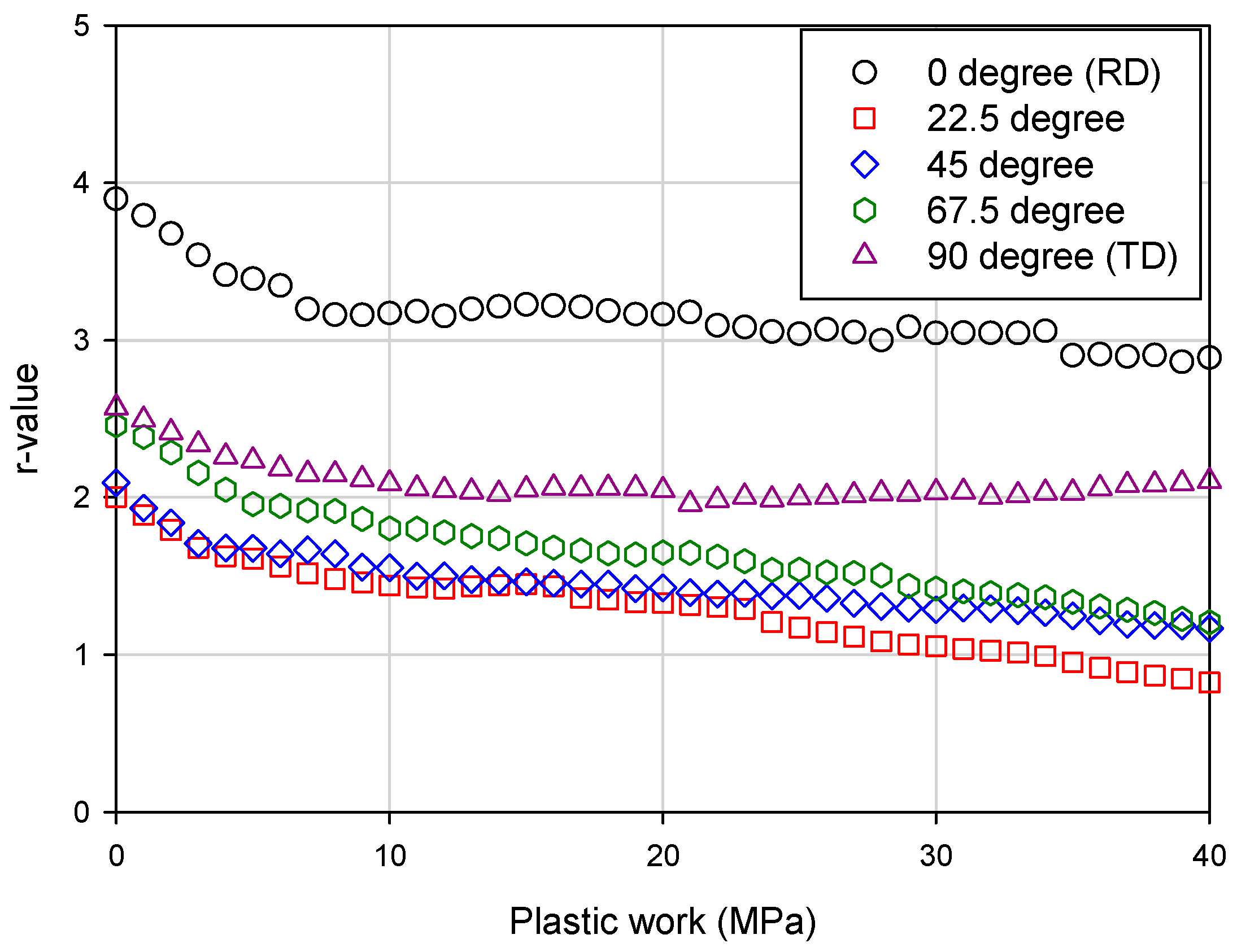
The evolutions of r-values for the Q&P 980 steel and niobium with respect to the plastic work are shown in Figure 3a and Figure 4, respectively.
As seen in Figure 3a, the measured r-values for the Q&P 980 steel stay almost constant for all directions as a function of the plastic work. The averaged r-values for the Q&P 980 steel are summarized in Table 1 and the directional distributions are shown in Figure 3b. Meanwhile, the measured r-values for the niobium sheet shows evidence of evolution during the plastic work as shown in Figure 4.
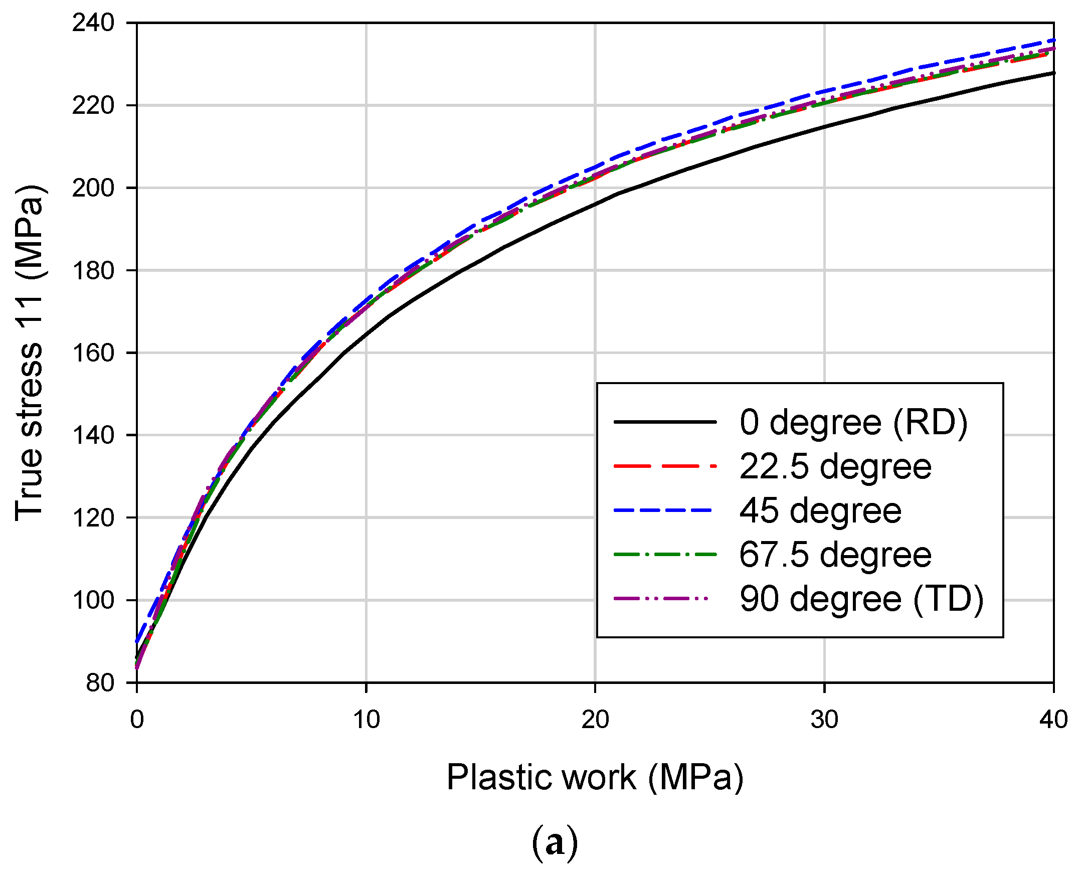
The evolution of yield stress with respect to plastic work for each tensile direction was also characterized from the uniaxial tension test data as shown in Figure 5 and Figure 6, for the Q&P 980 steel and niobium sheet, respectively. In Figure 5b and Figure 6b, the yield stress evolution for each direction was normalized by the yield stress along the rolling direction in order to clearly compare the directional difference. For the niobium sheet, the hydraulic bulge test was conducted at constant true thickness strain rate of 0.005/s. The true thickness strain was converted into the plastic thickness strain by eliminating the elastic thickness strain and the yield stress evolution was calibrated based on the plastic work shown in Figure 6.
3. Non-Associated Flow Rule Based on Plastic Work
Based on the normality rule, the plastic strain increment is obtained by:
where g(σ) is the n-th order homogeneous plastic potential function and dλ is the Lagrangian multiplier.
The yield criterion to define the anisotropic yield stress is:
where f is the m-th order homogeneous yield stress function and is the effective yield stress to describe the hardening evolution. In this work, the hardening evolution of the effective yield stress is defined based on the plastic work, , instead of the accumulated equivalent plastic strain, . The equivalent plastic strain increment, , is conjugated quantity to the effective yield stress, , and defined from the following plastic work equivalence principle [18,33]:
Here, is the equivalent plastic strain increment conjugated to the effective stress, , which determines the normalized size of the n-th order homogeneous plastic potential function, g(σ); i.e.,
The following relationships between the effective quantities can be derived from Equation (4):
and
Since g(σ) is the n-th order homogeneous function, Equation (4) becomes by substituting Equation (2):
Therefore,
The co-rotational objective stress rate of the Cauchy stress from the linear elastic constitutive law is:
where is the fourth order elastic stiffness tensor, dε is the total strain increment, dεe is the elastic strain increment, and dεp is the plastic strain increment. From Equations (2) and (9), the stress increment becomes,
From Equation (3), the following relationship is obtained:
By substituting Equation (11) into Equation (12),
Therefore,
and
The elasto-plastic tangent modulus is obtained by substituting Equation (14) or (15) into Equation (11):
Note that the elasto-plastic tangent modulus in Equation (16) is asymmetric when the plastic potential function is different from the yield function. In order to make symmetric tangent modulus, the equivalent plastic strain increments and need to be obtained, similar to the derivations in Equations (12) and (13), by manipulating the relationship in Equation (5):
and
Then, the following symmetric elasto-plastic stiffness modulus [18] can be obtained by substituting Equation (17) or (18) into Equation (11):
Here, can be determined from the rate of the prescribed hardening evolution, , by manipulating Equations (16) and (19):
The numerical implementation of the plastic work based developed evolutionary yield function is described in Appendix A.
4. Assumed Anisotropic Yield and Potential Functions and Hardening Evolution Model
4.1. Evolutionary Yld2000-2d Function
In this work, the plane stress yield stress function Yld2000-2d proposed by Barlat et al. [3] was utilized for the description of the plastic potential function and the yield function. In the Yld2000-2d function, the yield function is defined as:
where
and
Here, and (k = I, II) are the principal values of the deviatoric stress tensor ( or ), which is obtained by the linear transformation of the Cauchy stress tensor, σ:
Here, the eight independent anisotropic coefficients of L′ and L″ are expressed as:
and
4.2. Calibration of the Evolutionary Yld2000-2d Functions
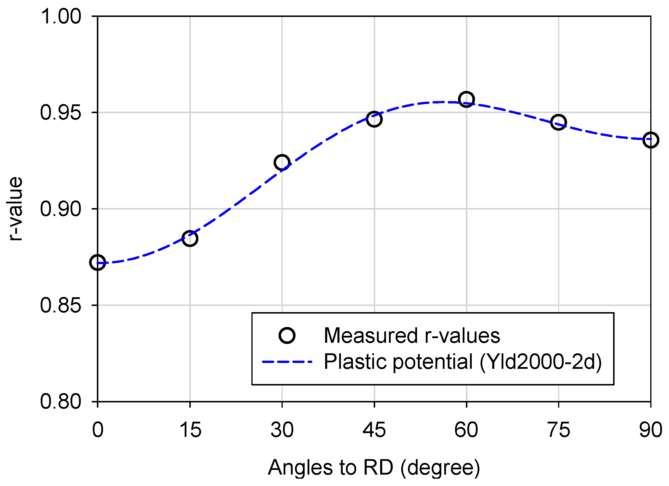
In the non-associated flow rule, the plastic potential and yield stress functions can either be selectively evolved or left as constants, depending upon the experimental data and the desired accuracy. For example, as shown in Figure 3a, the measured r-values for the Q&P 980 steel remain almost constant for all directions as a function of plastic work. Therefore, the measured r-value for each direction was assumed to be constant (e.g., non-evolving) for the Q&P 980 steel; i.e., we only considered the stationary plastic potential. Specifically, the averaged r-value for each tensile direction was utilized for the characterization of the plastic potential function, . In addition to the seven averaged r-values obtained from the uniaxial tension test data, the uniaxial tensile yield stress (YS in Table 1) along the rolling direction was used for the characterization of the eight coefficients of the plastic potential function. The calibrated parameters for the plastic potential are summarized in Table 3. Based on the calibrated plastic potential function, r-value distributions were calculated and compared with the measured r-values in Figure 7.
As seen in Figure 5b, the flow stress for the Q&P 980 steel varies as a function of plastic work. Therefore, to capture the evolution of the anisotropy, the parameters of the yield function were calibrated for every 5 MPa increment of the plastic work. Specifically, for the calibration of the eight coefficients of the Yld2000-2d function, we used seven yield stresses from the uniaxial tension data and the yield stress for the balanced biaxial tension, which was assumed to have the same value as the uniaxial tensile yield stress along the rolling direction. The calibrated parameters are summarized in Table 4.
The following asymptotic equation was used to evolve the yield function parameters, αj (j = 1~8), as a function of plastic work:
Here, ω is the plastic work, and are the initial values and changes of the yield function parameters, respectively, while and are the parameters to control the evolution speed. In order to avoid divergence of the yield function parameters beyond the characterization region, the evolution equation was designed to have an asymptotic evolution. The evolution coefficient was set to 1.0 for the simplicity of calibration for the Q&P 980 steel in this work. For general application, the evolution equation can be further generalized by adding exponential terms:
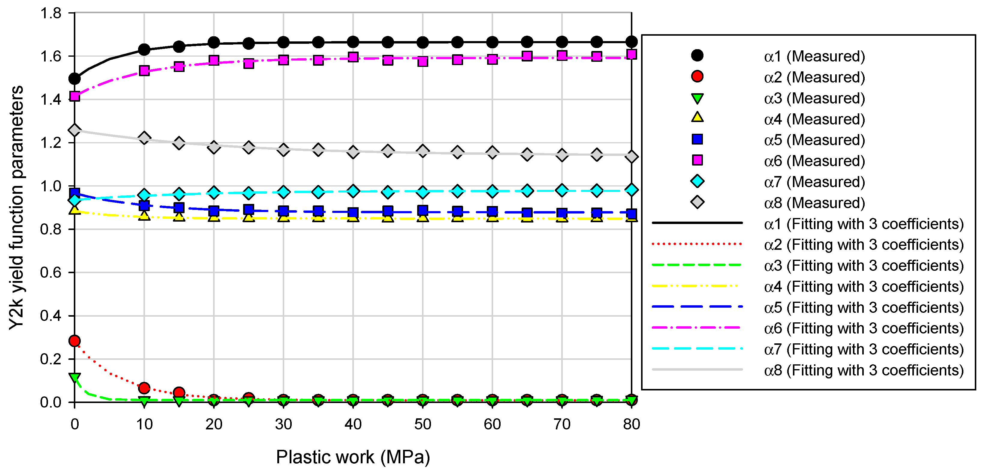
The calibrated evolution coefficients for each yield function parameter are summarized in Table 5 for the Q&P 980 steel. As seen in Figure 8, Equation (27) accurately captures the evolution of the yield function parameters as a function of plastic work.
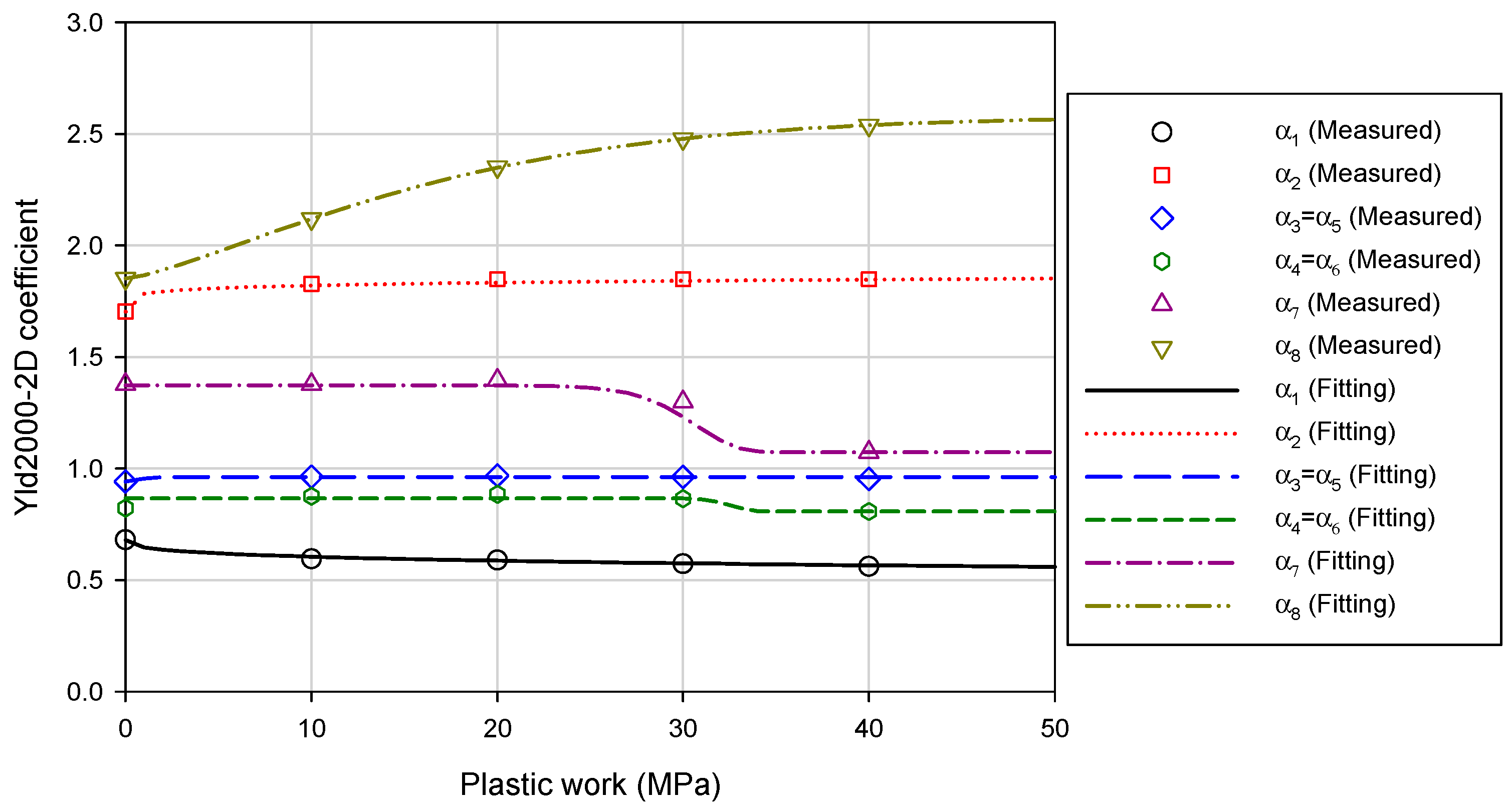
As seen in Figure 4 and Figure 6, unlike the Q&P 980 steel, the niobium sheet showed evolving anisotropy of r-values and flow stresses as a function of plastic work. Therefore, the parameters of the plastic potential function and yield function for the niobium sheet were calibrated for every 10 MPa increment of the plastic work. Specifically, five r-values and the uniaxial tension yield stress in the rolling direction were used to calibrate the potential function for niobium. As for the yield function, the five uniaxial tension yield stresses, and the balanced biaxial yield stress obtained from the hydraulic bulge test were used for calibration. For the niobium sheet, to utilize the six available experimental data for the calibration of the plastic potential function and yield function, the independent parameters of the Yld2000-2d function were reduced from eight to six by assuming α3 = α5 and α4 = α6. This simplified the linear transformation () of the deviatoric stress in Equation (26) as following:
Table 6 and Table 7 summarize the calibrated parameters for the yield function and plastic potential function, respectively.
The evolution of the parameters as a function of plastic work was captured using Equation (27) for the niobium sheet. The evolution coefficients for the plastic potential and yield function are summarized in Table 8 and Table 9, respectively. Figure 9 and Figure 10 show how Equation (27) accurately captures the evolution of the plastic potential function and the yield function parameters as a function of plastic work.
4.3. Isotropic Hardening Evolution
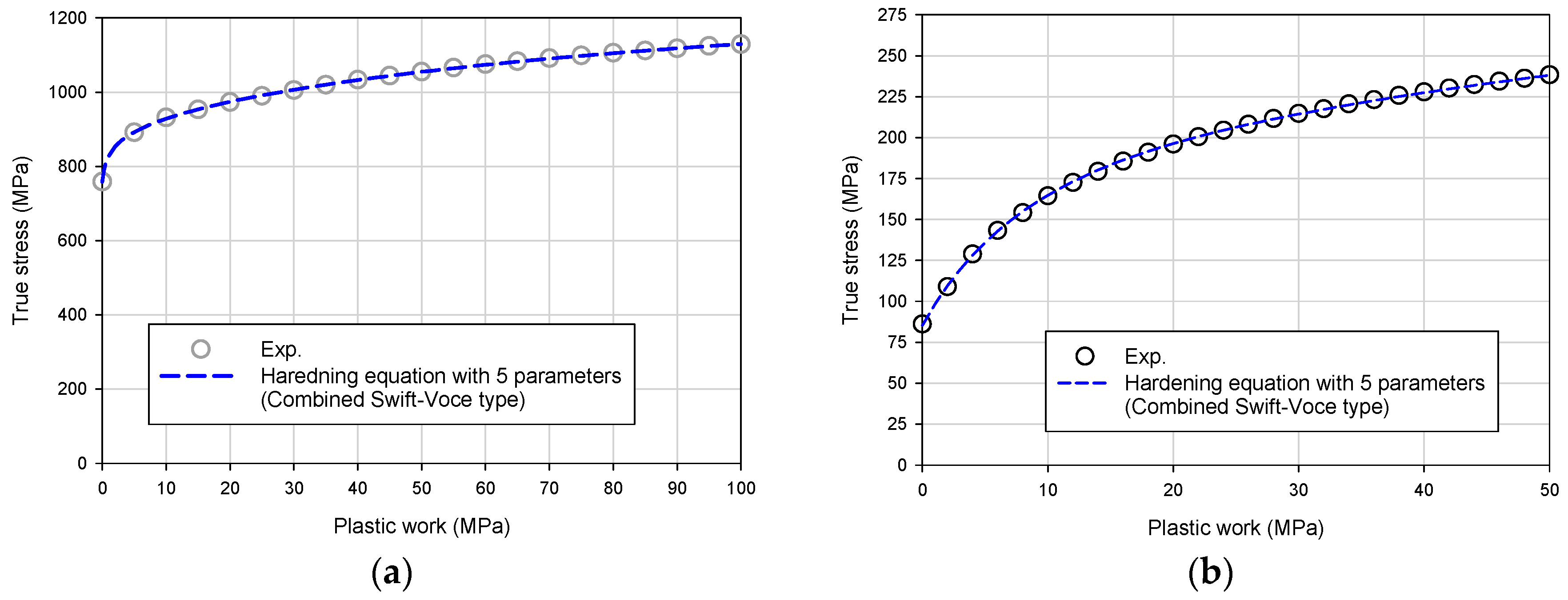
Full isotropic hardening (expansion of the yield surface without translation) of the Q&P 980 steel and niobium sheet was characterized based on the uniaxial tension test data. Since the evolution of the yield function was characterized and described by the plastic work, the hardening behavior was also described by the plastic work using the following combined Swift–Voce type hardening rule by selecting the uniaxial tension data along the rolling direction as a reference state:
where , ω0, nω, , and cω are hardening coefficients, ω is the accumulated plastic work (), and is the normalization coefficient that makes the quantity in the bracket unit less.
The calibrated hardening coefficients for the combined Swift–Voce type hardening rule are summarized in Table 10. The hardening evolution of the Q&P 980 steel and niobium sheet with respect to the plastic work was calculated based on the calibrated hardening coefficients and compared with the measured hardening curve in Figure 11.
4.4. Predicted Evolution of Yield and Plastic Potential Functions as a Function of Plastic Work
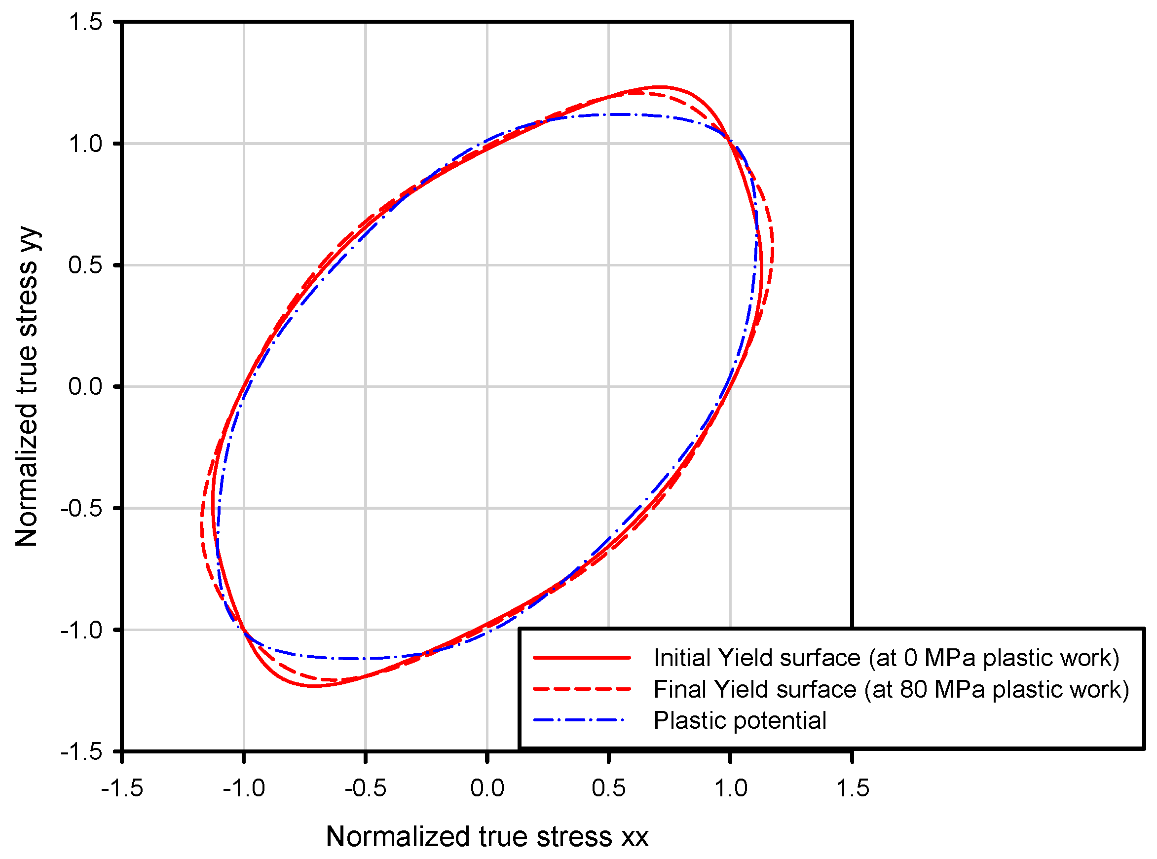
Based on the calibrated evolution coefficients of the yield function for the Q&P 980 steel, the initial yield surface at 0 MPa plastic work and the final yield surface (at 80 MPa plastic work) normalized by the yield stress along the rolling direction are compared with the contour of the plastic potential in Figure 12. It should be noted that the potential function was assumed to not evolve since the r-values were assumed to remain constant as a function of plastic work.
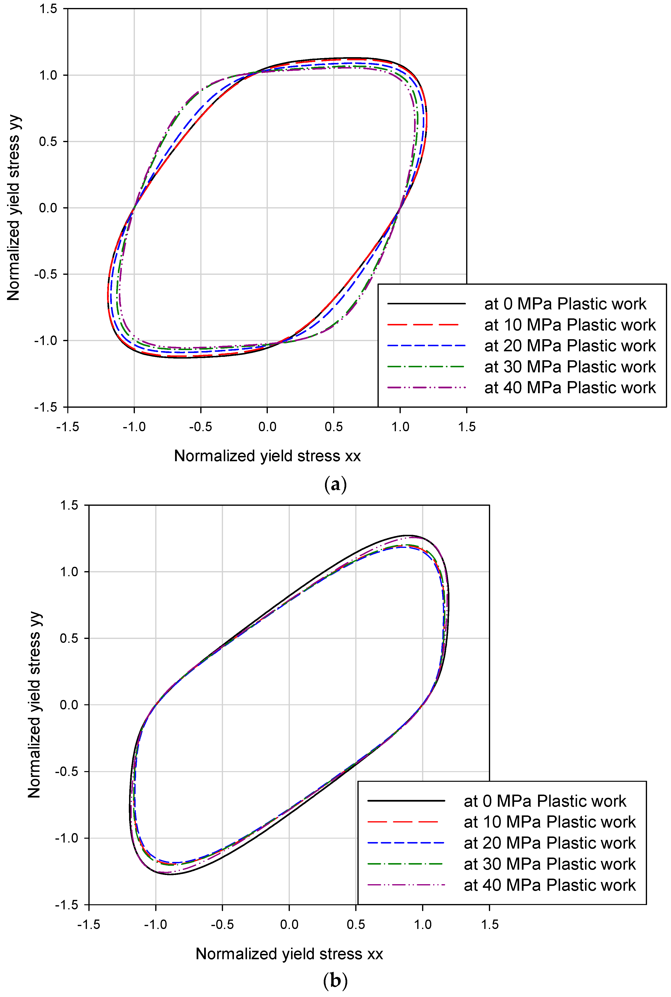
The expansion of the yield surfaces at every 10 MPa increment of the plastic work was calculated for the niobium sheet. For comparison, the contours of the normalized yield surfaces and plastic potential surfaces at every 10 MPa increment of the plastic work were calculated. Comparison of Figure 13 clearly shows that the yield and plastic potential functions evolve differently as a function of plastic work.
To guarantee the uniqueness of the solution, the denominators in Equations (14) and (15) must be positive. This satisfies the stability constraint suggested by Stoughton and Yoon [13,15]. Since the hardening evolution term, , and the effective stresses, and , are always non-negative, the stability constraint is satisfied when is positive. To demonstrate the stability of the proposed model based on the evolutionary non-associated yield function, the evolution of was calculated for the niobium sheet. As shown in Figure 14, for both the 0 MPa plastic work and 40 MPa plastic work cases, the tensor product always remains positive for all available stress modes under the plane stress condition.
5. Comparison of Evolutionary and Non-Evolutionary Yield Function Models
5.1. Uniaxial Tension Test
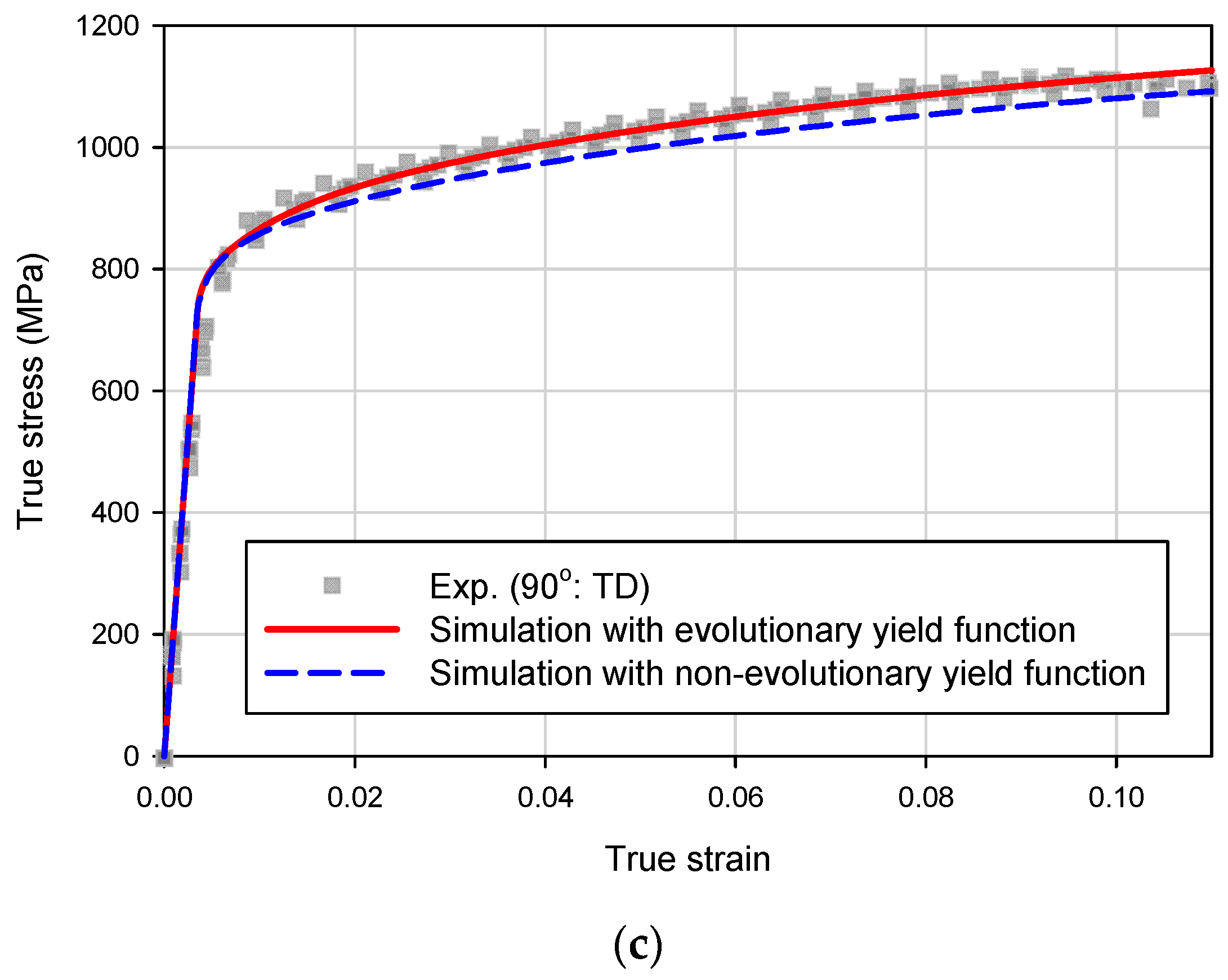
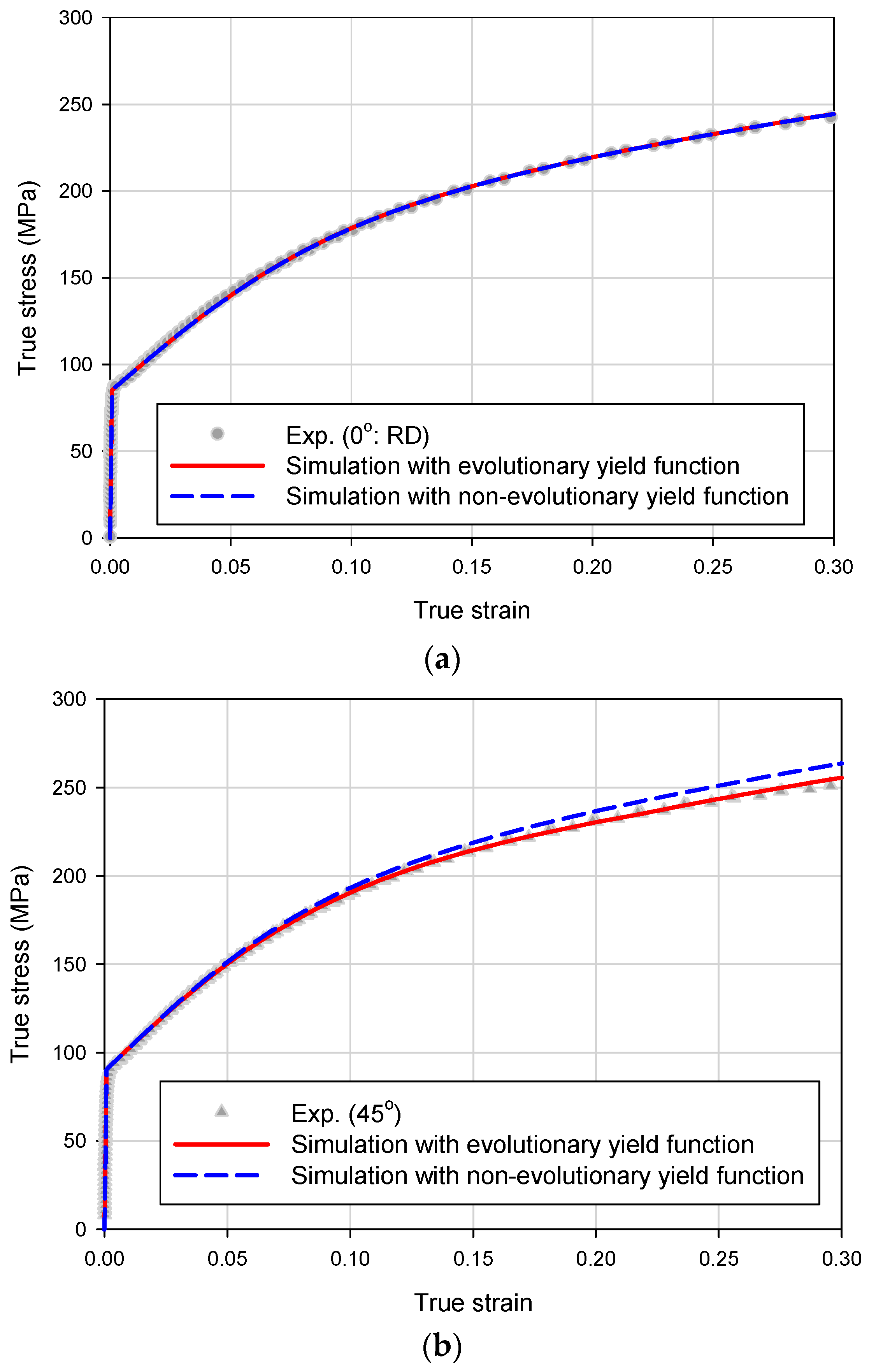
For the verification of the effect of the evolution of yield and plastic potential functions, uniaxial tension simulations were performed for the Q&P 980 steel and niobium sheet using the developed evolutionary yield function model. Tensile directions considered for the simulations were 0, 45, and 90 degrees off the rolling direction. The characterized evolutionary yield functions and plastic potentials (summarized in Table 5, Table 8, and Table 9), as well as the isotropic hardening rule based on the plastic work (summarized in Table 10) were employed for the tensile simulations. For comparison, an isotropic hardening model without the evolution of the yield function and the plastic potential (labeled as non-evolutionary yield function) was also considered for simulations. The initial yield surface and plastic potential at 0 MPa plastic work were considered for the non-evolving yield surface and plastic potential, respectively. The simulated true stress–strain curves for the Q&P 980 steel and niobium sheet are compared with experiments in Figure 15 and Figure 16, respectively. Both the evolutionary yield function and non-evolutionary yield function models accurately predicted the stress–strain curves in the rolling direction as shown in Figure 15a and Figure 16a. However, in the simulations for the directions in 45 and 90 degrees off the rolling direction, only the evolutionary yield function model accurately predicted stress–strain curves. Compared with the experiments, the non-evolutionary yield function model accurately predicted the initial yield stresses but showed gradual deviations in the prediction of the subsequent stress–strain curves.
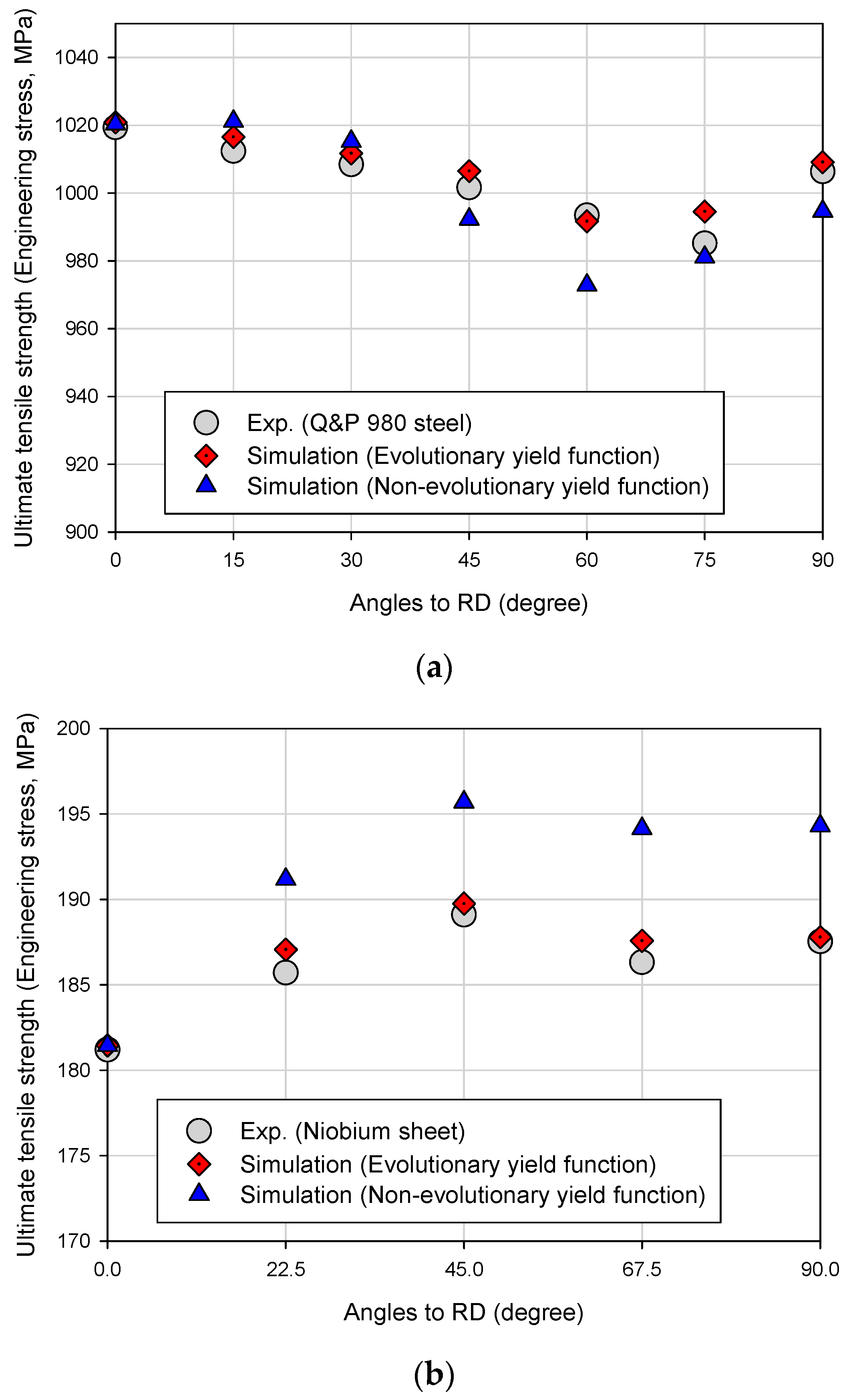
Besides the true stress–strain curves, the simulated ultimate tensile strengths (UTS) along different tensile directions (off the rolling direction) were compared with experiments. As shown in the comparison of the measured and calculated ultimate tensile strengths in Figure 17a,b for the Q&P 980 steel and niobium sheet, respectively, the simulation results considering the evolution of the yield function show much better agreement with experiments compared with those without evolving the yield function and plastic potential.
5.2. Prediction of Earing Profiles in Cup Drawing
In order to evaluate the effect of the initial anisotropy and its evolution in sheet forming simulations, the cylindrical cup drawing test was considered. Since experimental results were not available for the cup drawing test, the earing profiles were instead predicted using an analytical model [34]. To evaluate the capability of the non-associated flow rule to describe anisotropy, anisotropic yield functions under the associated flow rule were additionally considered for the description of the initial anisotropy and the anisotropy after evolution.
The analytical model [34] to predict the earing profile assumes that the blank in the flange area undergoes near plane strain deformation. For simplicity, simple compression mode in the circumferential direction is assumed in the flange area. From the force equilibrium condition along the circumferential direction, the vertical wall height, , is derived:
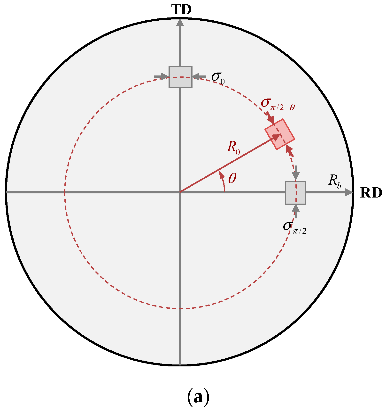
Here, is the total radial true strain, and are the r-value and yield stress along the direction, respectively, while is the average compressive yield stress. As schematically shown in Figure 18, , , and are the radial distance from the center of the initial blank, initial radius of the blank, and the radius of the cup, respectively. Detailed derivations are described in [34].
The radius to create the cup bottom and corner from the initial blank, , is obtained by applying the incompressibility condition for the volume of the cup corner:
where, Rp is the punch bottom radius, rp is the punch corner radius, and t0 is the initial thickness of the blank. Then, the total cup height is obtained by:
As for the representation of the anisotropy, non-quadratic anisotropic yield functions, Yld2000-2D and CPB06 [6] functions under the associated flow rule were additionally considered. As proposed by Plunkett et al. [35], the CPB06 function can be extended by incorporating multiple linear stress transformations for better accuracy; i.e.:
where is,
Here, is the asymmetry coefficient, while , , and are the principal values of the transformed stress, . The linear transformation is defined as:
where and are the fourth-order orthotropic linear transformation tensor.
From the CPB06ex3 function [35], which has three linear stress transformations, 21 independent coefficients for the plane stress condition were reduced to 12 independent coefficients by introducing the following constraints to guarantee the deviatoric stress components in the linear transformation:
Here, , , , and are the anisotropy coefficients for (p)-th linear transformation. Since three linear stress transformations were considered and each transformation requires four independent coefficients, a total of twelve anisotropy coefficients exist for the description of the anisotropy. The anisotropic/asymmetric yield function reduces to isotropic function, when the anisotropy coefficients are equal to one and the asymmetry coefficients are zero.
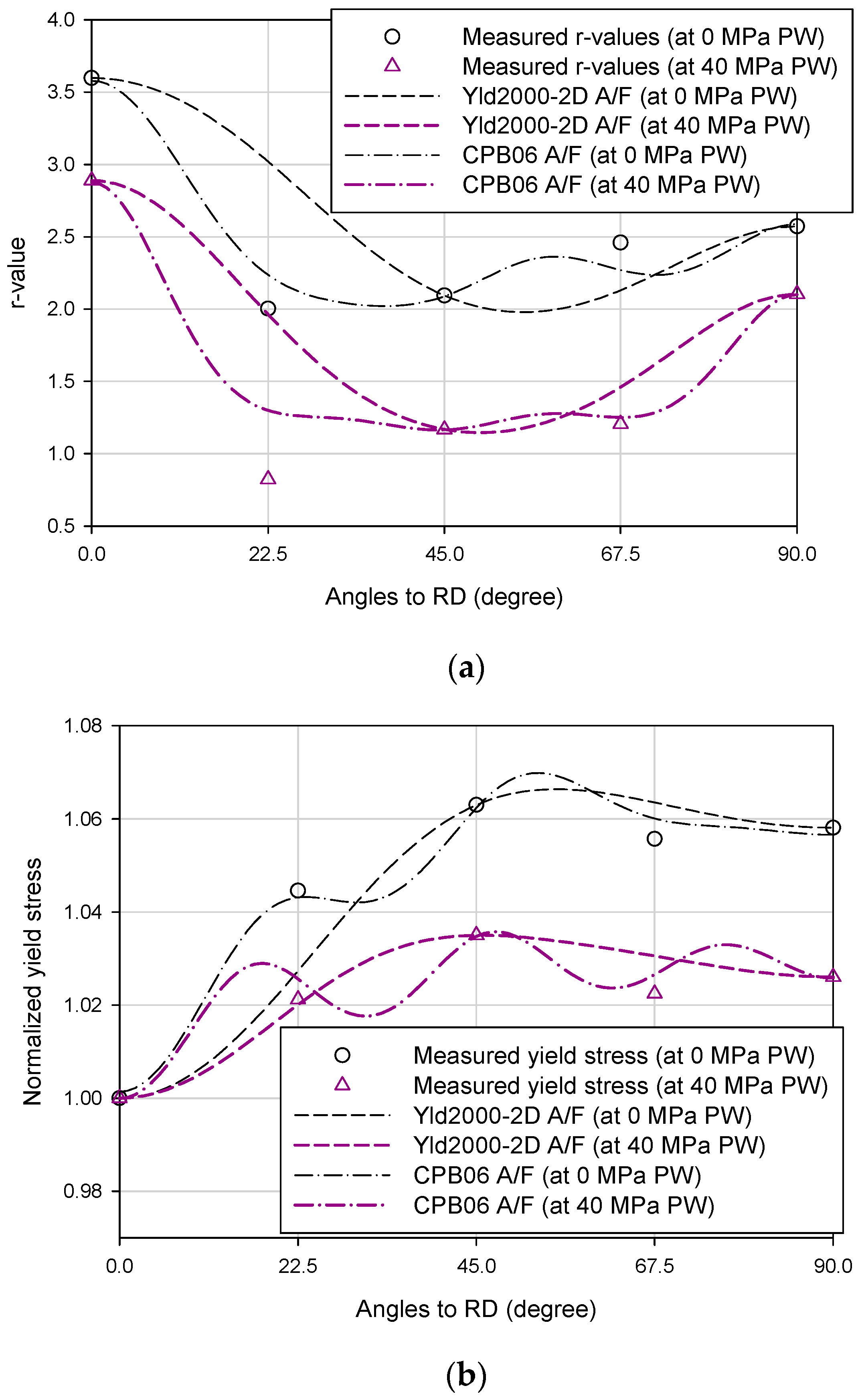
As for the calibration of the anisotropy coefficients for the Yld2000-2D function and the modified CPB06ex3 function under the associated flow rule, the niobium sheet, which shows severe anisotropy, was considered. To evaluate the impact of anisotropic evolution, the initial anisotropy (at 0 MPa of the accumulated plastic work) and the anisotropy after evolution (at 40 MPa of the accumulated plastic work) were considered. Similar to the calibration of yield functions and plastic potentials for the non-associated flow rule, the yield stresses and r-values in the uniaxial tension tests as well as the balanced biaxial tension test were utilized to calibrate the Yld2000-2D and the CPB06ex3 functions under the associated flow rule. To determine the eight and twelve anisotropy coefficients, three r-values (in 45 degree increments) and five tensile stresses (in 22.5 degree increments) were considered for the Yld2000-2D and the CPB06ex3 functions, respectively. Asymmetry was ignored for simplicity in the CPB06ex3 function, and isotropy was assumed for the r-values in the balanced biaxial tension; i.e., and rb = 1.0. The calibrated anisotropy coefficients for the Yld2000-2D and the CPB06ex3 functions are summarized in Table 11 and Table 12, respectively.
The calculated r-values and yield stresses from the calibrated associated flow rule (Yld2000-2D function and CPB06ex3 function as shown in Figure 19) were also used for the prediction of the cup height profiles. As separately compared in Figure 20b,c, the predicted height profiles based on the CPB06ex3 function under the associated flow rule show overall good agreement with the prediction based on the experimental data. Note that twelve independent coefficients were employed to account for the anisotropy both for the CPB06ex3 function under the associated flow rule and the Yld2000-2D function under the non-associated flow rule (6 coefficients for each yield function and plastic potential). The predicted profiles based on the Yld2000-2D function under the associated flow rule show some differences from the prediction based on experimental data, since insufficient number of anisotropy coefficients were employed to account for the severe anisotropy of the niobium sheet. As more anisotropy coefficients were employed for the description of the anisotropy, the predicted profiles showed better agreements with the predicted profiles directly obtained from the experimental r-values and yield stresses.
6. Conclusions
A constitutive law was developed based on the evolutionary yield function to account for the evolution of anisotropy induced by the plastic deformation. Based on the non-associated flow rule, the yield stress function and the plastic potential were separately defined for the effective description of anisotropy. The anisotropic evolution of the yield stress function and the plastic potential were described by a general asymptotic evolution equation. As for the equivalent plastic status to define the plastic potential and yield stress function, as well as the hardening rule, the accumulated plastic work was employed as an alternative to the accumulated plastic strain. Inaccuracy and complexity in the material characterization can be avoided by the introduction of the plastic work, since the measured data must be converted into the equivalent quantities prior to the characterization of the plastic potential and yield function. Numerical formulations based on the plastic work were also derived in case the hardening rule as well as the evolution of the plastic potential and the yield stress function are defined in terms of the accumulated plastic work.
For the validation of the developed constitutive law, mechanical properties of the BAO Q&P 980 steel and niobium sheets at room temperature were characterized from uniaxial tensile tests as well as the balanced biaxial tension test. From the experimental data, separate sets of the anisotropic coefficients for each of the plastic potential and yield stress function were obtained as a function of the plastic work. For a general description of the evolutions of the yield function and plastic potential as well as to reduce the number of coefficients, the measured sets of the anisotropic coefficients were fit to a general asymptotic evolution equation. Through comparison with non-evolutionary yield functions in the prediction of the ultimate tensile strength in different tensile directions and the earing profiles in the cup drawing test, the importance of the developed constitutive law to properly describe the evolution of the plastic potential and yield function was proven, particularly for the niobium sheet, which exhibits highly anisotropic behavior.
Author Contributions
Conceptualization, T.P.; methodology, T.P.; software, T.P.; validation, T.P.; formal analysis, T.P.; investigation, T.P.; resources, F.A.-F. and F.P.; data curation, T.P.; writing—original draft preparation, T.P. and F.P.; writing—review and editing, T.P. and F.P.; visualization, T.P.; supervision, F.P.; project administration, F.P.; funding acquisition, F.P.
Funding
This research was funded by the U.S. Department of Energy through the DOE award DE-FG02-13ER41974. Also, this material is based upon work supported by the Department of Energy under Cooperative Agreement Number DOE DE-EE000597, with United States Automotive Materials Partnership LLC (USAMP).
Acknowledgments
The authors wish to thank the U.S. Department of Energy for the support of this project through the DOE award DE-FG02-13ER41974 and DOE DE-EE000597, with United States Automotive Materials Partnership LLC (USAMP). This report was prepared as an account of work sponsored by an agency of the United States Government. Neither the United States Government nor any agency thereof, nor any of their employees, makes any warranty, express or implied, or assumes any legal liability or responsibility for the accuracy, completeness, or usefulness of any information, apparatus, product, or process disclosed, or represents that its use would not infringe privately owned rights. Reference herein to any specific commercial product, process, or service by trade name, trademark, manufacturer, or otherwise does not necessarily constitute or imply its endorsement, recommendation, or favoring by the United States Government or any agency thereof. The views and opinions of authors expressed herein do not necessarily state or reflect those of the United States Government or any agency thereof.
Conflicts of Interest
The authors declare no conflict of interest. The funders had no role in the design of the study; in the collection, analyses, or interpretation of data; in the writing of the manuscript, or in the decision to publish the results.
Appendix A
In this work, the predictor–corrector scheme [36,37] was employed for the numerical implementation of the developed evolutionary yield function model based on the plastic work.
From a given discrete strain increment, (), the trial Cauchy stress is initially updated by assuming purely elastic step and preserving the state variables from the previous n-th discretized time step ( and ):
Here, the superscript, k, denotes the iteration number (: trial step), while the subscripts, and , denote the discrete time step number.
The next (n + 1)-th step is purely elastic if the following yield condition is satisfied:
Otherwise, the ()-th step is elasto-plastic. Then, the plastic work, , and the Cauchy stress, , should be iteratively updated until the following consistency condition is satisfied:
where
Here, Tol is the tolerance, which is numerically infinitesimal value to guarantee the solution accuracy.
The equivalent plastic strain increments, plastic work, and Cauchy stress are iteratively updated until the consistency condition in Equation (A3) is satisfied.
The increment of the equivalent plastic strain is calculated by:
The denominator, , can be decomposed by the chain rule:
Here,
From Equation (11):
If the elastic stiffness modulus, , is evolving as a function of the plastic work, ignoring the second order variations, Equation (A10) becomes:
Then, the equivalent plastic strain increments are updated:
and
Then, the accumulated plastic work is updated based on the plastic work equivalence principle in Equation (4):
From Equation (A11), the Cauchy stress is updated by,
References
- Hill, R. A theory of the yielding and plastic flow of anisotropic metals. Proc. R. Soc. Lond. Ser. A Math. Phys. Sci. 1948, 193, 281–297. [Google Scholar] [Green Version]
- Barlat, F.; Maeda, Y.; Chung, K.; Yanagawa, M.; Brem, J.C.; Hayashida, Y.; Lege, D.J.; Matsui, K.; Murtha, S.J.; Hattori, S.; et al. Yield function development for aluminum alloy sheets. J. Mech. Phys. Solids 1997, 45, 1727–1763. [Google Scholar] [CrossRef]
- Barlat, F.; Brem, J.C.; Yoon, J.W.; Chung, K.; Dick, R.E.; Lege, D.J.; Pourboghrat, F.; Choi, S.H.; Chu, E. Plane stress yield function for aluminum alloy sheets—Part 1: Theory. Int. J. Plast. 2003, 19, 1297–1319. [Google Scholar] [CrossRef]
- Barlat, F.; Aretz, H.; Yoon, J.W.; Karabin, M.E.; Brem, J.C.; Dick, R.E. Linear transfomation-based anisotropic yield functions. Int. J. Plast. 2005, 21, 1009–1039. [Google Scholar] [CrossRef]
- Banabic, D.; Aretz, H.; Comsa, D.S.; Paraianu, L. An improved analytical description of orthotropy in metallic sheets. Int. J. Plast. 2005, 21, 493–512. [Google Scholar] [CrossRef]
- Cazacu, O.; Plunkett, B.; Barlat, F. Orthotropic yield criterion for hexagonal closed packed metals. Int. J. Plast. 2006, 22, 1171–1194. [Google Scholar] [CrossRef]
- Aretz, H.; Barlat, F. New convex yield functions for orthotropic metal plasticity. Int. J. Non-Linear Mech. 2013, 51, 97–111. [Google Scholar] [CrossRef]
- Yoshida, F.; Hamasaki, H.; Uemori, T. A user-friendly 3D yield function to describe anisotropy of steel sheets. Int. J. Plast. 2013, 45, 119–139. [Google Scholar] [CrossRef]
- Karafillis, A.P.; Boyce, M.C. A general anisotropic yield criterion using bounds and a transformation weighting tensor. J. Mech. Phys. Solids 1993, 41, 1859–1886. [Google Scholar] [CrossRef]
- Drucker, D.C. A Definition of Stable Inelastic Material. J. Appl. Mech. 1959, 26, 101–106. [Google Scholar]
- Stoughton, T.B. A non-associated flow rule for sheet metal forming. Int. J. Plast. 2002, 18, 687–714. [Google Scholar] [CrossRef]
- Lademo, O.G.; Hopperstad, O.S.; Langseth, M. Evaluation of yield criteria and flow rules for aluminum alloys. Int. J. Plast. 1999, 15, 191–208. [Google Scholar] [CrossRef]
- Stoughton, T.B.; Yoon, J.W. Review of Drucker’s postulate and the issue of plastic stability in metal forming. Int. J. Plast. 2006, 22, 391–433. [Google Scholar] [CrossRef]
- Cvitanić, V.; Vlak, F.; Lozina, Ž. A finite element formulation based on non-associated plasticity for sheet metal forming. Int. J. Plast. 2008, 24, 646–687. [Google Scholar] [CrossRef]
- Stoughton, T.B.; Yoon, J.W. On the existence of indeterminate solutions to the equations of motion under non-associated flow. Int. J. Plast. 2008, 24, 583–613. [Google Scholar] [CrossRef]
- Stoughton, T.B.; Yoon, J.W. Anisotropic hardening and non-associated flow in proportional loading of sheet metals. Int. J. Plast. 2009, 25, 1777–1817. [Google Scholar] [CrossRef]
- Taherizadeh, A.; Green, D.E.; Ghaei, A.; Yoon, J.W. A non-associated constitutive model with mixed iso-kinematic hardening for finite element simulation of sheet metal forming. Int. J. Plast. 2010, 26, 288–309. [Google Scholar] [CrossRef]
- Park, T.; Chung, K. Non-associated flow rule with symmetric stiffness modulus for isotropic-kinematic hardening and its application for earing in circular cup drawing. Int. J. Solids Struct. 2012, 49, 3582–3593. [Google Scholar] [CrossRef] [Green Version]
- Taherizadeh, A.; Green, D.E.; Yoon, J.W. A non-associated plasticity model with anisotropic and nonlinear kinematic hardening for simulation of sheet metal forming. Int. J. Solids Struct. 2015, 69–70, 370–382. [Google Scholar] [CrossRef]
- Spitzig, W.A.; Sober, R.J.; Richmond, O. Pressure dependence of yielding and associated volume expansion in tempered martensite. Acta Metall. 1975, 23, 885–893. [Google Scholar] [CrossRef]
- Zamiri, A.R.; Pourboghrat, F. A novel yield function for single crystals based on combined constraints optimization. Int. J. Plast. 2010, 26, 731–746. [Google Scholar] [CrossRef]
- Hill, R.; Hutchinson, J.W. Differential Hardening in Sheet Metal Under Biaxial Loading: A Theoretical Framework. J. Appl. Mech. 2008, 59, S1. [Google Scholar] [CrossRef]
- Abedrabbo, N.; Pourboghrat, F.; Carsley, J. Forming of aluminum alloys at elevated temperatures—Part 1: Material characterization. Int. J. Plast. 2006, 22, 314–341. [Google Scholar] [CrossRef]
- Abedrabbo, N.; Pourboghrat, F.; Carsley, J. Forming of aluminum alloys at elevated temperatures—Part 2: Numerical modeling and experimental verification. Int. J. Plast. 2006, 22, 342–373. [Google Scholar] [CrossRef]
- Plunkett, B.; Cazacu, O.; Lebensohn, R.A.; Barlat, F. Elastic-viscoplastic anisotropic modeling of textured metals and validation using the Taylor cylinder impact test. Int. J. Plast. 2007, 23, 1001–1021. [Google Scholar] [CrossRef]
- Zamiri, A.; Pourboghrat, F. Characterization and development of an evolutionary yield function for the superconducting niobium sheet. Int. J. Solids Struct. 2007, 44, 8627–8647. [Google Scholar] [CrossRef] [Green Version]
- Aretz, H. A simple isotropic-distortional hardening model and its application in elastic-plastic analysis of localized necking in orthotropic sheet metals. Int. J. Plast. 2008, 24, 1457–1480. [Google Scholar] [CrossRef]
- Chung, K.; Park, T. Consistency condition of isotropic-kinematic hardening of anisotropic yield functions with full isotropic hardening under monotonously proportional loading. Int. J. Plast. 2013, 45, 61–84. [Google Scholar] [CrossRef]
- Yoshida, F.; Hamasaki, H.; Uemori, T. Modeling of anisotropic hardening of sheet metals including description of the Bauschinger effect. Int. J. Plast. 2015, 75, 170–188. [Google Scholar] [CrossRef]
- Park, T.; Hector, L.G.; Hu, X.; Abu-Farha, F.; Fellinger, M.R.; Kim, H.; Esmaeilpour, R.; Pourboghrat, F. Crystal Plasticity Modeling of 3rd Generation Multi-phase AHSS with Martensitic Transformation. Int. J. Plast. 2019, in press. [Google Scholar] [CrossRef]
- Abu-Farha, F.; Hu, X.; Sun, X.; Ren, Y.; Hector, L.G.; Thomas, G.; Brown, T.W. In Situ Local Measurement of Austenite Mechanical Stability and Transformation Behavior in Third-Generation Advanced High-Strength Steels. Metall. Mater. Trans. A 2018, 49, 2583–2596. [Google Scholar] [CrossRef]
- Zamiri, A.; Pourboghrat, F.; Barlat, F. An effective computational algorithm for rate-independent crystal plasticity based on a single crystal yield surface with an application to tube hydroforming. Int. J. Plast. 2007, 23, 1126–1147. [Google Scholar] [CrossRef]
- Chung, K.; Lee, M.-G.; Kim, D.; Kim, C.; Wenner, M.L.; Barlat, F. Spring-back evaluation of automotive sheets based on isotropic-kinematic hardening laws and non-quadratic anisotropic yield functions. Int. J. Plast. 2005, 21, 861–882. [Google Scholar] [CrossRef]
- Chung, K.; Kim, D.; Park, T. Analytical derivation of earing in circular cup drawing based on simple tension properties. Eur. J. Mech. A/Solids 2011, 30, 275–280. [Google Scholar] [CrossRef]
- Plunkett, B.; Cazacu, O.; Barlat, F. Orthotropic yield criteria for description of the anisotropy in tension and compression of sheet metals. Int. J. Plast. 2008, 24, 847–866. [Google Scholar] [CrossRef]
- Chung, K. The Analysis of Anisotropic Hardening in Finite-Deformation Plasticity. Ph.D. Thesis, Stanford University, Stanford, CA, USA, 1984. [Google Scholar]
- Simo, J.C.; Hughes, T.J.R. Interdisciplinary Applied Mathematics—Computational Inelasticity; Springer: Berlin, Germany, 2013; Volume 7, ISBN 4420767936. [Google Scholar]
Figure 1.
Comparison of the calculated yield surfaces based on crystal plasticity simulations and isotropic version of the Yld2000-2D function.
Figure 1.
Comparison of the calculated yield surfaces based on crystal plasticity simulations and isotropic version of the Yld2000-2D function.

Figure 2.
Comparison of the calculated strain-rate potentials based on crystal plasticity simulations and isotropic version of the Yld2000-2D function.
Figure 2.
Comparison of the calculated strain-rate potentials based on crystal plasticity simulations and isotropic version of the Yld2000-2D function.

Figure 3.
Measured r-values for the QP980 steel averaged from 5 experiments for each tensile direction: (a) evolutions with respect to plastic work; (b) averaged r-value distributions.
Figure 3.
Measured r-values for the QP980 steel averaged from 5 experiments for each tensile direction: (a) evolutions with respect to plastic work; (b) averaged r-value distributions.


Figure 4.
Evolution of the r-values for the niobium sheet averaged from 3 experiments for each tensile direction.
Figure 4.
Evolution of the r-values for the niobium sheet averaged from 3 experiments for each tensile direction.

Figure 5.
Measured (a) yield stress and (b) normalized yield stress evolutions for the Q&P 980 steel with respect to the plastic work.
Figure 5.
Measured (a) yield stress and (b) normalized yield stress evolutions for the Q&P 980 steel with respect to the plastic work.

Figure 6.
Measured (a) yield stress and (b) normalized yield stress evolutions for the niobium sheet with respect to the plastic work.
Figure 6.
Measured (a) yield stress and (b) normalized yield stress evolutions for the niobium sheet with respect to the plastic work.


Figure 7.
Comparison of the averaged r-values for the Q&P 980 steel and the calculated distribution based on the plastic potential function.
Figure 7.
Comparison of the averaged r-values for the Q&P 980 steel and the calculated distribution based on the plastic potential function.

Figure 8.
Evolutions of the parameters of the yield function (Yld2000-2d function) for the Q&P 980 steel with respect to the plastic work.
Figure 8.
Evolutions of the parameters of the yield function (Yld2000-2d function) for the Q&P 980 steel with respect to the plastic work.

Figure 9.
Evolutions of the parameters of the plastic potential function (Yld2000-2d function) for the niobium sheet with respect to the plastic work.
Figure 9.
Evolutions of the parameters of the plastic potential function (Yld2000-2d function) for the niobium sheet with respect to the plastic work.

Figure 10.
Evolutions of the parameters of yield function (Yld2000-2d function) for the niobium sheet with respect to the plastic work.
Figure 10.
Evolutions of the parameters of yield function (Yld2000-2d function) for the niobium sheet with respect to the plastic work.

Figure 11.
Comparison of the measured and calculated hardening behavior of (a) the QP980 steel and (b) niobium sheet with respect to the plastic work.
Figure 11.
Comparison of the measured and calculated hardening behavior of (a) the QP980 steel and (b) niobium sheet with respect to the plastic work.

Figure 12.
Comparison of the normalized contours of the yield functions (at 0 MPa and 80 MPa of the plastic work) and plastic potential function for the Q&P 980 steel.
Figure 12.
Comparison of the normalized contours of the yield functions (at 0 MPa and 80 MPa of the plastic work) and plastic potential function for the Q&P 980 steel.

Figure 13.
Comparison of the normalized contours of (a) the yield functions and (b) plastic potential function for the niobium sheet.
Figure 13.
Comparison of the normalized contours of (a) the yield functions and (b) plastic potential function for the niobium sheet.

Figure 14.
The tensor product of the gradients of the yield function and the plastic potential for the elastic stiffness tensor for the niobium sheet (a) at 0 MPa plastic work and (b) at 40 MPa plastic work.
Figure 14.
The tensor product of the gradients of the yield function and the plastic potential for the elastic stiffness tensor for the niobium sheet (a) at 0 MPa plastic work and (b) at 40 MPa plastic work.

Figure 15.
Comparison of the measured and simulated true stress–strain curves for (a) 0, (b) 45 and (c) 90 degrees off tensile directions for the Q&P 980 steel.
Figure 15.
Comparison of the measured and simulated true stress–strain curves for (a) 0, (b) 45 and (c) 90 degrees off tensile directions for the Q&P 980 steel.


Figure 16.
Comparison of the measured and simulated true stress–strain curves for (a) 0, (b) 45 and (c) 90 degrees off tensile directions for the niobium sheet.
Figure 16.
Comparison of the measured and simulated true stress–strain curves for (a) 0, (b) 45 and (c) 90 degrees off tensile directions for the niobium sheet.


Figure 17.
Comparison of the measured and simulated ultimate tensile strength (UTS) distributions for (a) the Q&P 980 steel and (b) niobium sheet.
Figure 17.
Comparison of the measured and simulated ultimate tensile strength (UTS) distributions for (a) the Q&P 980 steel and (b) niobium sheet.

Figure 18.
A schematic view of the initial circular blank and drawn cup: (a) top view of the initial blank and material element in the flange area; (b) cross-section view of the initial blank and the final cup.
Figure 18.
A schematic view of the initial circular blank and drawn cup: (a) top view of the initial blank and material element in the flange area; (b) cross-section view of the initial blank and the final cup.


Figure 19.
Comparison of the measured and calculated (a) r-values and (b) normalized yield stresses based on associated flow rule (Yld2000-2D and CPB06ex3 yield functions) for the niobium sheet.
Figure 19.
Comparison of the measured and calculated (a) r-values and (b) normalized yield stresses based on associated flow rule (Yld2000-2D and CPB06ex3 yield functions) for the niobium sheet.

Figure 20.
Comparison of the predicted cup height profiles: (a) based on the non-associated flow rule with Yld2000-2D functions; (b) based on the associated flow rule with Yld2000-2D and CPB06ex3 functions at 0 MPa of the accumulated plastic work; (c) based on the associated flow rule with Yld2000-2D and CPB06ex3 functions at 40 MPa of the accumulated plastic work.


Table 1.
Measured elastic and plastic properties of the Q&P980 steel.
| Degree | E (GPa) | YS (MPa) | UE (true) | UE (eng) | UTS (MPa) | TE (eng) |
|---|---|---|---|---|---|---|
| 0 | 212.72 | 814.29 ± 14.58 | 0.1015 ± 0.0050 | 10.68% | 1019.3 ± 13.85 | 15.49% |
| 15 | 212.12 | 809.03 ± 9.94 | 0.0984 ± 0.0036 | 10.34% | 1012.4 ± 13.92 | 14.67% |
| 30 | 201.53 | 809.38 ± 19.74 | 0.0989 ± 0.0089 | 10.39% | 1008.5 ± 9.40 | 14.85% |
| 45 | 211.57 | 783.78 ± 22.71 | 0.1004 ± 0.0043 | 10.56% | 1001.6 ± 14.41 | 14.49% |
| 60 | 210.20 | 776.23 ± 13.88 | 0.0925 ± 0.0059 | 9.69% | 993.48 ± 12.07 | 13.69% |
| 75 | 211.89 | 753.75 ± 15.83 | 0.0972 ± 0.0029 | 10.20% | 985.20 ± 2.92 | 14.41% |
| 90 | 214.40 | 783.82 ± 18.94 | 0.0904 ± 0.0042 | 9.46% | 1006.4 ± 15.69 | 13.14% |
Table 2.
Measured elastic and plastic properties of the niobium sheet.
| Degree | E (GPa) | YS (MPa) | UE (true) | UE (eng) | UTS (MPa) | TE (eng) |
|---|---|---|---|---|---|---|
| 0 | 109.178 | 86.12 ± 0.46 | 0.2871 ± 0.0233 | 32.07% | 181.20 ± 1.01 | 50.55% |
| 22.5 | 104.075 | 89.96 ± 0.43 | 0.2536 ± 0.0149 | 28.88% | 185.71 ± 0.61 | 48.54% |
| 45 | 106.635 | 91.55 ± 0.20 | 0.2551 ± 0.0225 | 29.05% | 189.11 ± 1.20 | 49.91% |
| 67.5 | 108.396 | 90.92 ± 0.49 | 0.2577 ± 0.0133 | 29.40% | 186.32 ± 0.30 | 50.08% |
| 90 | 109.475 | 91.12 ± 0.34 | 0.2485 ± 0.0127 | 28.21% | 187.54 ± 0.46 | 50.06% |
Table 3.
Calibrated parameters for the plastic potential of the Q&P 980 steel (m = 6) based on the averaged r-values.
Table 3.
Calibrated parameters for the plastic potential of the Q&P 980 steel (m = 6) based on the averaged r-values.
| α1 | α2 | α3 | α4 | α5 | α6 | α7 | α8 |
|---|---|---|---|---|---|---|---|
| 1.0206 | 0.9604 | 1.0120 | 0.9991 | 1.0104 | 0.9284 | 1.0088 | 1.0689 |
Table 4.
Calibrated parameters for the yield function of the Q&P 980 steel (m = 6).
| Plastic Work | α1 | α2 | α3 | α4 | α5 | α6 | α7 | α8 |
|---|---|---|---|---|---|---|---|---|
| 0 MPa | 1.4953 | 0.2830 | 0.1191 | 0.8849 | 0.9671 | 1.4143 | 0.9344 | 1.2582 |
| 10 MPa | 1.6297 | 0.0653 | 0.0105 | 0.8574 | 0.9093 | 1.5329 | 0.9581 | 1.2221 |
| 15 MPa | 1.6430 | 0.0434 | 0.0100 | 0.8530 | 0.8997 | 1.5515 | 0.9629 | 1.1979 |
| 20 MPa | 1.6632 | 0.0103 | 0.0100 | 0.8520 | 0.8848 | 1.5801 | 0.9696 | 1.1785 |
| 25 MPa | 1.6578 | 0.0177 | 0.0101 | 0.8512 | 0.8922 | 1.5657 | 0.9667 | 1.1777 |
| 30 MPa | 1.6632 | 0.0101 | 0.0100 | 0.8504 | 0.8841 | 1.5814 | 0.9721 | 1.1668 |
| 35 MPa | 1.6634 | 0.0101 | 0.0101 | 0.8503 | 0.8842 | 1.5813 | 0.9719 | 1.1671 |
| 40 MPa | 1.6648 | 0.0100 | 0.0100 | 0.8503 | 0.8770 | 1.5956 | 0.9771 | 1.1566 |
| 45 MPa | 1.6633 | 0.0101 | 0.0101 | 0.8496 | 0.8843 | 1.5812 | 0.9711 | 1.1620 |
| 50 MPa | 1.6626 | 0.0101 | 0.0101 | 0.8502 | 0.8874 | 1.5749 | 0.9707 | 1.1623 |
| 55 MPa | 1.6634 | 0.0100 | 0.0101 | 0.8506 | 0.8833 | 1.5830 | 0.9757 | 1.1561 |
| 60 MPa | 1.6636 | 0.0100 | 0.0101 | 0.8502 | 0.8826 | 1.5845 | 0.9755 | 1.1549 |
| 65 MPa | 1.6650 | 0.0100 | 0.0101 | 0.8495 | 0.8748 | 1.6001 | 0.9783 | 1.1452 |
| 70 MPa | 1.6652 | 0.0100 | 0.0101 | 0.8498 | 0.8738 | 1.6021 | 0.9802 | 1.1426 |
| 75 MPa | 1.6650 | 0.0101 | 0.0113 | 0.8503 | 0.8758 | 1.5980 | 0.9787 | 1.1447 |
| 80 MPa | 1.6658 | 0.0103 | 0.0125 | 0.8509 | 0.8702 | 1.6091 | 0.9831 | 1.1354 |
Table 5.
Evolution coefficients for the parameters of the yield function of the Q&P 980 steel.
| Coefficients | α1 | α2 | α3 | α4 | α5 | α6 | α7 | α8 |
|---|---|---|---|---|---|---|---|---|
| 1.4953 | 0.2831 | 0.1191 | 0.8849 | 0.9664 | 1.4156 | 0.9357 | 1.2585 | |
| 0.1690 | −0.2736 | −0.1088 | −0.0348 | −0.0877 | 0.1764 | 0.0422 | −0.1168 | |
| 0.1548 | 0.1569 | 0.6777 | 0.1582 | 0.0991 | 0.1019 | 0.0654 | 0.0464 | |
| 1.0 | 1.0 | 1.0 | 1.0 | 1.0 | 1.0 | 1.0 | 1.0 |
Table 6.
Calibrated parameters for the plastic potential function of the niobium sheet for every 10 MPa increments of the plastic work (m = 6).
Table 6.
Calibrated parameters for the plastic potential function of the niobium sheet for every 10 MPa increments of the plastic work (m = 6).
| Plastic Work | α1 | α2 | α3 | α4 | α5 | α6 | α7 | α8 |
|---|---|---|---|---|---|---|---|---|
| 0 MPa | 0.6807 | 1.7038 | 0.9417 | 0.8227 | 0.9417 | 0.8227 | 1.3780 | 1.8533 |
| 10 MPa | 0.5951 | 1.8291 | 0.9640 | 0.8757 | 0.9640 | 0.8757 | 1.3779 | 2.1203 |
| 20 MPa | 0.5890 | 1.8500 | 0.9695 | 0.8843 | 0.9695 | 0.8843 | 1.3977 | 2.3527 |
| 30 MPa | 0.5728 | 1.8500 | 0.9627 | 0.8652 | 0.9627 | 0.8652 | 1.2995 | 2.4792 |
| 40 MPa | 0.5607 | 1.8500 | 0.9531 | 0.8073 | 0.9531 | 0.8073 | 1.0729 | 2.5402 |
Table 7.
Calibrated parameters for the yield function of the niobium sheet for every 10 MPa increments of the plastic work (m = 6).
Table 7.
Calibrated parameters for the yield function of the niobium sheet for every 10 MPa increments of the plastic work (m = 6).
| Plastic Work | α1 | α2 | α3 | α4 | α5 | α6 | α7 | α8 |
|---|---|---|---|---|---|---|---|---|
| 0 MPa | 1.3006 | 0.6013 | 0.9172 | 0.9921 | 0.9172 | 0.9921 | 0.8118 | 1.0749 |
| 10 MPa | 1.3123 | 0.5903 | 0.9157 | 1.0030 | 0.9157 | 1.0030 | 0.8047 | 1.1019 |
| 20 MPa | 1.3986 | 0.4090 | 0.9277 | 1.0297 | 0.9277 | 1.0297 | 0.8134 | 1.0825 |
| 30 MPa | 1.5755 | 0.0302 | 0.9481 | 1.0517 | 0.9481 | 1.0517 | 0.7514 | 1.0980 |
| 40 MPa | 1.5521 | 0.0307 | 0.9730 | 1.0626 | 0.9730 | 1.0626 | 0.7511 | 1.0953 |
Table 8.
Evolution coefficients for the parameters of the plastic potential of the niobium sheet.
| Plastic Work | α1 | α2 | α3 | α4 | α5 | α6 | α7 | α8 |
|---|---|---|---|---|---|---|---|---|
| 0.6804 | 1.7038 | 0.9417 | 0.8669 | 0.9417 | 0.8669 | 1.3741 | 1.8533 | |
| −0.2266 | 0.2566 | 0.0203 | −0.0596 | 0.0203 | −0.0596 | −0.3012 | 0.7275 | |
| 0.0100 | 0.0100 | 0.9982 | 0.0305 | 0.9982 | 0.0305 | 0.0324 | 0.0555 | |
| 0.3916 | 0.2100 | 1.8879 | 40.3301 | 1.8879 | 40.3301 | 15.3666 | 1.3290 |
Table 9.
Evolution coefficients for the parameters of the yield function of the niobium sheet.
| Plastic Work | α1 | α2 | α3 | α4 | α5 | α6 | α7 | α8 |
|---|---|---|---|---|---|---|---|---|
| 1.3044 | 0.5965 | 0.9146 | 0.9899 | 0.9146 | 0.9899 | 0.8094 | 1.0725 | |
| 0.2594 | −0.5671 | 0.0905 | 0.0773 | 0.0905 | 0.0773 | −0.0583 | 0.0219 | |
| 0.0446 | 0.0434 | 0.0253 | 0.0424 | 0.0253 | 0.0424 | 0.0339 | 0.9989 | |
| 6.9800 | 6.4951 | 2.7805 | 1.9661 | 2.7805 | 1.9661 | 14.4294 | 2.9090 |
Table 10.
Calibrated combined Swift–Voce type isotropic hardening coefficients for the Q&P 980 steel and niobium sheet.
Table 10.
Calibrated combined Swift–Voce type isotropic hardening coefficients for the Q&P 980 steel and niobium sheet.
| Material | (MPa) | ω0 (MPa) | nω | (MPa) | cω |
|---|---|---|---|---|---|
| Q&P 980 | 820.91 | 0.1690 | 0.0441 | 182.77 | 0.0114/MPa |
| Niobium | 57.6062 | 3.8927 | 0.2885 | 56.1982 | 0.1365/MPa |
Table 11.
Calibrated anisotropy coefficients for the Yld2000-2D function of the niobium sheet under the associated flow rule (m = 6).
Table 11.
Calibrated anisotropy coefficients for the Yld2000-2D function of the niobium sheet under the associated flow rule (m = 6).
| Plastic Work | ||||||||
|---|---|---|---|---|---|---|---|---|
| 0 MPa | 1.2256 | 0.8647 | 0.8873 | 0.8925 | 0.8764 | 1.2586 | 0.9963 | 0.7654 |
| 40 MPa | 1.1606 | 0.9500 | 1.0490 | 0.9484 | 0.9391 | 1.2765 | 0.9883 | 0.8631 |
Table 12.
Calibrated anisotropy coefficients for the CPB06ex3 function of the niobium sheet under the associated flow rule (m = 6).
Table 12.
Calibrated anisotropy coefficients for the CPB06ex3 function of the niobium sheet under the associated flow rule (m = 6).
| Plastic Work | Transformation Tensor | a(p) | b(p) | c(p) | d(p) |
|---|---|---|---|---|---|
| 0 MPa | 0.0329 | −0.0311 | 0.5825 | 0.823 | |
| −0.1657 | 0.1856 | 1.5469 | 0.8169 | ||
| 1.2197 | −1.6697 | 0.4713 | 0.9273 | ||
| 40 MPa | −0.0884 | 0.0937 | 1.5509 | 0.5428 | |
| 0.9958 | 0.8517 | −0.2335 | 0.479 | ||
| 1.4769 | −1.6672 | 0.1893 | 1.0092 |
© 2019 by the authors. Licensee MDPI, Basel, Switzerland. This article is an open access article distributed under the terms and conditions of the Creative Commons Attribution (CC BY) license (http://creativecommons.org/licenses/by/4.0/).
Share and Cite
MDPI and ACS Style
Park, T.; Abu-Farha, F.; Pourboghrat, F. An Evolutionary Yield Function Model Based on Plastic Work and Non-Associated Flow Rule. Metals 2019, 9, 611. https://doi.org/10.3390/met9050611
AMA Style
Park T, Abu-Farha F, Pourboghrat F. An Evolutionary Yield Function Model Based on Plastic Work and Non-Associated Flow Rule. Metals. 2019; 9(5):611. https://doi.org/10.3390/met9050611
Chicago/Turabian StylePark, Taejoon, Fadi Abu-Farha, and Farhang Pourboghrat. 2019. "An Evolutionary Yield Function Model Based on Plastic Work and Non-Associated Flow Rule" Metals 9, no. 5: 611. https://doi.org/10.3390/met9050611
Note that from the first issue of 2016, this journal uses article numbers instead of page numbers. See further details here.