Comparison of Experimental Thermal Methods for the Fatigue Limit Evaluation of a Stainless Steel

Abstract

This paper regards the rapid determination of fatigue limit by using thermal data analysis. Different approaches available in the literature to estimate the fatigue limit of cold-drawn AISI 304L bars are analyzed and compared, namely, temperature- and energy-based methods. Among the temperature-based approaches, the Risitano Method (RM) and the method based on material temperature evolution recorded during a static tensile test were analyzed. Regarding the energy-based approaches, the input mechanical energy density stored in the material per cycle (i.e., the area of the hysteresis loop), the heat energy dissipated by the material to the surroundings per cycle, and the “2nd-harmonic-based” methods were considered. It was found that for the material analyzed, all the considered energy-based approaches provided a very good engineering estimation of the material fatigue limit compared to a staircase test.

1. Introduction

Fatigue is an irreversible process, accompanied by microstructural changes, localized plastic strains, and energy dissipation. The temperature rise of a metallic material undergoing a fatigue test is a manifestation of the thermal energy dissipation, and it was experimentally observed that the higher the applied stress amplitude, the more pronounced the temperature increase of the material. Moreover, the trend of the observed temperature increase versus the applied stress amplitude presents a relatively abrupt change at a certain stress level. This characteristic stress amplitude is associated with the material fatigue limit [1,2,3,4,5,6,7]. Since the load-increasing tests are fast and a single specimen can be used to estimate the material fatigue limit, Risitano and co-workers set up a rapid experimental methodology (i.e., the Risitano Method) to determine the fatigue limit based on load-increasing tests on specimens monitored with an infrared camera [5]. Recently, Risitano and Risitano [8] proposed an even faster experimental approach to estimate the material fatigue limit, consisting in monitoring the material temperature during a simple static tensile test.

Krapez et al. [9] proposed adopting lock-in thermography to rapidly evaluate the material fatigue limit. In fact, they noticed that the temperature oscillations related to plasticity effects, i.e., characterised by double frequency of the load signal, ΔT_D, exhibit improved correlation with the fatigue limit as compared to the material temperature. However, they noticed that the applicability of the method depends on the material under analysis. In particular, satisfactory results were found for AISI 1050 steel and AISI 316L stainless steel, while the approach was ineffective when investigating the fatigue behavior of 7010 aluminium alloy, since the temperature signal associated with the dissipated energy was very weak in relation to the available experimental equipment.

Akai et al. [10] proposed the use of the dissipated thermal energy q, evaluated by using the conventional lock-in thermography, to assess the material fatigue limit. In fact, in their study [10], it was noticed that the q-σ_a trend shows an abrupt increase when the applied stress amplitude is higher than the fatigue limit. The authors proposed calculating q from the density of the material, ρ, its specific heat, c, and the material temperature variation due to plasticity ΔT_D, which is measured by using the conventional lock-in thermography. They pointed out that satisfactory results were found in the case of AISI 316L, while in the case of AISI 304, the fatigue limit estimated by dissipated energy measurements provided a conservative value as compared to that evaluated by means of conventional staircase fatigue tests.

The phase difference Δθ = θ_D − θ_E was proposed as a suitable damage index for the rapid determination of material fatigue limit by Shiozawa et al. [11]. θ_D was defined as the phase lag between the temperature change due to plasticity and the reference signal, and θ_E as the phase lag between the thermoelastic temperature and the cyclic load due to thermal diffusion. The authors noticed that Δθ assumed a characteristic value, $\Delta {\widehat{\mathsf{\theta }}}_{\mathrm{D}}$, when a large dissipated energy was observed. On the basis of this experimental evidence, they proposed a “phase lock-in method” to calculate the dissipated energy $\widehat{q}$, by taking into account the $\Delta {\widehat{\mathsf{\theta }}}_{\mathrm{D}}$ value, as will be shown later. Their approach was validated by experimental results obtained from AISI 306L stainless-steel specimens, carrying out push–pull fatigue tests by imposing a sinusoidal load with a test frequency of 5 Hz. The authors noticed a satisfactory agreement with the fatigue limit determined by the conventional staircase tests. Recently, Shiozawa et al. [12] extended the “phase lock-in method”, assuming the increasing rate of the dissipated energy, $\mathrm{d}\widehat{q}/\mathrm{d}{\mathsf{\sigma }}_{\mathrm{a}}$, as the fatigue index. By plotting $\mathrm{d}\widehat{q}/\mathrm{d}{\mathsf{\sigma }}_{\mathrm{a}}$ versus σ_a, an abrupt increase is seen when σ_a exceeds the material fatigue limit.

The Thermoelastic Phase Analysis (TPA) was proposed by Palumbo and Galietti to rapidly evaluate the fatigue limit of martensitic steels [13]. The authors proposed an accurate experimental procedure to evaluate the evolution of the thermoelastic phase (defined as the phase lag between the thermoelastic temperature, i.e., the first harmonic of the temperature signal, and the load signal) along a step-load fatigue test, carried out by imposing a nominal load ratio R = 0.5 (R defined as the ratio between the minimum and the maximum stress values reached during the load cycle, i.e., R = σ_min/σ_max) and test frequency equal to 17 Hz. They pointed out that the thermoelastic phase plotted versus the applied stress amplitude shows an abrupt change when the fatigue limit is exceeded.

Some years ago, Meneghetti [14] proposed an experimental technique for the direct evaluation of the heat energy density per cycle dissipated by a material undergoing a fatigue test (the $\overline{Q}$ parameter), on which the material temperature depends. $\overline{Q}$ can be easily evaluated by stopping the fatigue test at t = t* after thermal equilibrium has been reached and by measuring the cooling gradient immediately after t*. The $\overline{Q}$ parameter was initially adopted to rationalize in a single scatter band approximately 160 experimental results generated from constant-amplitude, completely reversed, stress- or strain-controlled fatigue tests on plain or notched hot-rolled stainless-steel specimens, having notch radii r_n = 3, 5, and 8 mm [15,16] and r_n = 0.5, 1, and 3 mm [17,18], as well as from tests on cold drawn un-notched bars of the same steel, under fully reversed axial or torsional fatigue loading conditions [19]. In view of this body of evidence, the $\overline{Q}$ parameter was proven to be an effective fatigue damage index. It is envisaged that the specific heat loss $\overline{Q}$ may be used also to estimate the fatigue limit.

This paper analyzes and compares some temperature- and energy-based approaches reported in the literature for an engineering estimation of the fatigue limit, defined in the Classical High-Cycle Fatigue regime. In particular, the rapid engineering techniques proposed by La Rosa and Risitano [5], by Risitano and Risitano [8], by Akai et al. [10], and by Shiozawa et al. [12], as well as the $\overline{Q}$ [14] parameter and the input mechanical energy density $\overline{W}$, stored in the material per cycle (i.e., the area of the hysteresis loop) [20] were applied to estimate the fatigue limit of cold-drawn AISI 304L stainless-steel bars. Critical issues applying the analyzed techniques were singled out. As a result, it was found that all the energy-based methods examined allowed the fatigue limit to be estimated with a very good level of accuracy as compared to the classical staircase procedure [21].

2. Experimental Approaches for the Rapid Estimation of Material Fatigue Limit

Concerning metallic materials, irreversible plastic deformations are responsible for crack initiation and its subsequent growth and may occur at a mesoscopic scale (i.e., the scale of grains) in the high-cycle fatigue regime [22]. The onset of non-recoverable plastic deformations during a fatigue test means that some energy consumption occurs in one load cycle. Of the total energy expended to repeatedly induce plastic deformations in a unit volume of material, only part is accumulated in the form of internal energy and is responsible for fatigue damage accumulation and final fracture. The remaining part is dissipated to the surroundings as heat [16,23]. According to Luong [4], it should be pointed out that the physical nature of fatigue damage should be distinguished by the phenomenon of heat dissipation, which is not by nature an indicator of fatigue damage. In fact, the fatigue damage consists in crack nucleation followed by crack propagation, which can lead to final failure. On the other hand, a temperature rise can be observed in a loaded specimen even below the fatigue limit, as a result of some anelastic dissipative phenomena that are not damaging as fatigue is. Nevertheless, there is a sufficient experimental evidence that the higher the plastic cyclic strains, which the fatigue strength depend on, the more intensive the heat energy dissipation.

According to the classical continuum mechanics reported in some studies [24,25], the energy balance equation can be written in terms of power per unit volume by introducing the Helmotz free energy as a thermodynamic potential [25,26,27,28]. If the power quantities appearing in the energy balance equation are averaged over one fatigue loading cycle, then we have [29] (the dot symbol indicates the time derivative):

$$\mathsf{\rho }c\dot{\overline{T}}-\mathsf{\lambda }{\nabla }^2\overline{T}=\dot{\overline{W}}-{\dot{\overline{E}}}_{\mathrm{s}}$$

(1)

where $\overline{W}$ is the plastic strain energy per cycle, ${\overline{E}}_{\mathrm{s}}$ is the stored energy per cycle, $\overline{T}$ is the average material temperature per cycle, $\mathsf{\lambda }$ is the coefficient of material thermal conductivity, ρ is the material density, and c is the material specific heat.

Equation (1) can be derived from the general energy balance equation, considering the following observations [29]:

• The contribution of the thermoelastic heat source in Equation (1) vanishes because it consists of a reversible exchange between mechanical and thermal energy, which does not produce a net energy dissipation or absorption over one loading cycle [30,31,32];
• The dependence of the material state on temperature is neglected, because temperature variations are small if compared to that necessary for phase transformation generating the coupling heat source in the form of latent heat.

By introducing the internal energy rate $\dot{\mathrm{U}}$ according to the definition given by Rousselier [27]:

$$\dot{U}=\rho \cdot c\cdot \dot{T}+{\dot{E}}_{\mathrm{s}}$$

(2)

If:

$$\dot{\overline{Q}}=\mathsf{\lambda }\cdot {\nabla }^2\overline{T}$$

(3)

then Equation (1) becomes:

$$\dot{\overline{U}}=\dot{\overline{W}}+\dot{\overline{Q}}$$

(4)

The energy balance Equation (4) is illustrated in Figure 1a, which shows the positive energy exchanges involved, i.e., the mechanical energy $\overline{W}$ and the heat energy $\overline{Q}$.

Since all energy contributions were averaged over one loading cycle, Equation (1) describes the evolution of the average temperature per cycle $\overline{T}(x,y,z;t)$, which is depicted in Figure 1b qualitatively. Then, the material temperature is related to the thermal energy dissipated in a unit volume of material per cycle (the parameter $\overline{Q}$), due to the fatigue process. Unfortunately, the temperature level reached by a material or a component during a constant amplitude fatigue test, characterized by a given amplitude, mean stress, and stress state, depends on the thermal and mechanical boundary conditions, such as the temperature of the surroundings, the specimen’s geometry, and the load test frequency. Conversely, $\overline{W}$ or $\overline{Q}$ are independent of the mechanical and thermal boundary conditions [15,24,33,34], (i.e., room temperature, specimen geometry, and test frequency [15]) but depend on the applied load cycle, defined by amplitude, mean value, and stress state [35]. In more details, in [15], a dedicated specimen made of AISI 304L was fatigued by imposing a constant stress amplitude, changing the mechanical and thermal boundary conditions. A first series of fatigue tests were carried out by imposing the load test frequency, f_L, from 2.5 to 9 Hz. Next, a second series of fatigue tests was conducted by imposing a constant f_L and by varying locally the heat transfer coefficient by means of either a blower or a heater, which directed the air flow towards the back face of the specimen. As expected, it was found that, despite the wide variation of the material temperature experimentally observed (up to 60 °C), the $\overline{Q}$ parameter (measured according to the experimental procedure described later on [14]) was contained within a scatter band equal to ±15% with respect to the mean value of $\overline{Q}$ measured during these fatigue tests. Finally, it was shown that, for a given test frequency, the $\overline{Q}$ values are within a scatter band equal to ±5% [15].

In the literature, different experimental approaches are available for the rapid evaluation of the material fatigue limit. The fatigue damage index is defined by the temperature in some studies and by the dissipated heat energy (on which the material temperature distribution depends on) in others. Therefore, depending on the variable considered as the fatigue damage index, the experimental approaches that were analyzed and discussed in this paper can be classified into temperature- and energy-based methods.

2.1. Temperature-Based Approaches

La Rosa and Risitano [5] proposed an experimental approach to rapidly evaluate the fatigue limit based on the experimental observation that a material undergoing a fatigue test is subjected to an increase of surface temperature, such that the higher the applied stress amplitude, the higher the temperature increase. In more detail, it was pointed out that when the applied stress amplitude σ_a is below the fatigue limit, the material temperature increase is extremely limited. On the contrary, when σ_a is higher than the fatigue limit, the material temperature rapidly increases at the beginning of the fatigue test and then stabilizes at a value ΔT_st when the thermal equilibrium with the surroundings is achieved, as sketched in Figure 2a. In view of this experimental evidence, it was proposed that the material fatigue limit can be evaluated by extrapolating down to zero the best fitting curve, which correlates ΔT_st to σ_a, as shown in Figure 2b. It is worth noting that the Risitano method (RM) is a rapid tool to estimate the material fatigue limit, since it requires the achievement of temperature stabilization and does not need to run the fatigue test until specimen failure. This thermometric approach is phenomenological and has been validated by means of a considerable number of experimental results.

Recently, Risitano and Risitano [8] proposed a new and even faster methodology to estimate the material fatigue limit by simply monitoring temperature evolution during a static tensile test. Their methodology is based on the hypothesis that fatigue failure occurs at the points where the local stress is able to produce plastic deformation, at least at a microscopic level. Therefore, the fatigue limit corresponds to the stress level, “σ_A,static”, which is responsible for local and irreversible plastic deformations. According to [8], since a static tensile test can be seen as part of the first cycle of a zero-mean stress fatigue test, the original authors argued that σ_A,static can be experimentally measured by monitoring the evolution of the surface material temperature during a static tensile test. In fact, the temperature-versus-stress plot is characterized by an initial linear trend due to the thermoelastic effect, followed by a loss of linearity due to the heat converted from the mechanical energy expected to induce the irreversible micro-plastic deformation. Following [8], σ_A,static is equal to the stress at the end of the linear trend of the temperature-versus-stress curve, as sketched in Figure 3.

2.2. Energy-Based Approaches

Meneghetti applied the first law of thermodynamics to a point on the specimen’s surface and averaged the energy quantities over one loading cycle [14].

When the temperature stabilizes, $\dot{\overline{T}}$ becomes null, therefore, through Equation (2), Equation (4) simplifies to:

$$\dot{\overline{W}}+\dot{\overline{Q}}={\dot{\overline{E}}}_{\mathrm{s}}$$

(5)

If the fatigue test is stopped suddenly at t = t* (Figure 4), then just after t* (i.e., at t = t*⁺), the mechanical input power $\dot{\overline{W}}$ as well as the rate of accumulation of fatigue damage ${\dot{\overline{E}}}_{\mathrm{s}}$ will become zero. By re-writing the energy balance equation Equation (4), one can obtain:

$$\dot{\overline{Q}}=\mathsf{\rho }·c·{\dot{T}|}_{t={\left(t^{*}\right)}^{+}}$$

(6)

It is worth noting that the heat energy rate $\dot{\overline{Q}}$ dissipated to the surroundings just before and just after t* is the same in Equations (5) and (6), because the temperature field is continuous through t*. Finally, the thermal energy released in a unit volume of material per cycle can be calculated by simply accounting for the load test frequency f_L [14,29,36,37]:

$$\overline{Q}=\frac{\dot{\overline{Q}}}{f_{\mathrm{L}}}=\frac{{\mathsf{\rho }\cdot c\cdot \dot{T}|}_{t={(t*)}^{+}}}{f_{\mathrm{L}}}$$

(7)

Equation (7) enables to perform in situ measurements of the specific heat loss $\overline{Q}$ at any point of a specimen or a component undergoing fatigue loading.

In this paper, $\overline{Q}$ and $\overline{W}$ were assumed as fatigue indexes able to rapidly estimate the material fatigue limit by step-load fatigue tests. It was envisaged that $\overline{W}$ or $\overline{Q}$ versus σ_a trends would exhibit an abrupt increase when σ_a was higher than the material fatigue limit, as shown in Figure 5a,b, respectively. As stated above, the main advantage of using $\overline{W}$ or $\overline{Q}$ with respect to temperature is that energy is independent of mechanical and thermal boundary conditions [15,24,33,34], (i.e., room temperature, specimen geometry, and test frequency [15]), while it depends on the applied load cycle, defined by amplitude, mean value, and stress state [35]. To exemplify, the curves reported in Figure 5a,b are thought of as material properties, as opposed to the curve reported in Figure 2b.

Shiozawa et al. [11] assumed that the dissipated thermal energy q can be calculated from the component of the temperature signal having double frequency with respect to the load signal sine wave. A discrete Fourier transform (DFT) can be applied to calculate the 2nd harmonic. In fact, during a single fatigue cycle, the material temperature oscillates because of the superposition of two different phenomena: the thermoelastic effect, which is a reversible phenomenon, and the irreversible energy dissipation caused by plastic deformation (see Figure 6). Once temperature stabilization is achieved, the energy dissipated over one cycle can be evaluated by considering the range of the second harmonic of the DFT of the temperature signal, ΔT_D, according to:

$$\Delta T_{\mathrm{D}}=2\sqrt{T_{\mathrm{D},\sin }^2+T_{\mathrm{D},\cos }^2}$$

(8)

where

$$T_{\mathrm{D},\sin }=\frac{2}{n}{\displaystyle \sum _{t_i=1}^{n}T\left(t_i\right)}\cdot \sin \left(2t_i\right)$$

(9a)

$$T_{\mathrm{D},\cos }=\frac{2}{n}{\displaystyle \sum _{t_i=1}^{n}T\left(t_i\right)}\cdot \cos \left(2t_i\right)$$

(9b)

where n is the number of recorded samples, and T(t_i) is the temperature signal measured at the time t_i.

Considering that during a zero-mean stress fatigue cycle, the effect of plasticity occurs twice, the dissipated thermal energy q can be calculated as follows [11]:

$$q=\mathsf{\rho }c\cdot 2\Delta T_{\mathrm{D}}$$

(10)

This approach was called the “conventional lock-in method” [11].

The phase lag between the temperature change due to energy dissipation and the load signal sine wave can be calculated as [11]:

$${\mathsf{\theta }}_{\mathrm{D}}={\tan }^{-1}\left(-\frac{T_{\mathrm{D},\cos }}{T_{\mathrm{D},\sin }}\right)$$

(11)

Since ${\mathsf{\theta }}_{\mathrm{D}}$ is influenced by thermal diffusion, the phase difference is defined to eliminate this influence, as follows [11]:

$$\Delta \mathsf{\theta }={\mathsf{\theta }}_{\mathrm{D}}-{\mathsf{\theta }}_{\mathrm{E}}$$

(12)

where ${\mathsf{\theta }}_{\mathrm{E}}$ is the phase lag between the thermoelastic temperature and the cyclic load due to the material thermal diffusivity and can be calculated according to Equation (13) [11]:

$${\mathsf{\theta }}_{\mathrm{E}}={\tan }^{-1}\left(-\frac{T_{\mathrm{E},\cos }}{T_{\mathrm{E},\sin }}\right)$$

(13)

where $T_{\mathrm{E},\sin }$ and $T_{\mathrm{E},\cos }$ are the components of the thermoelastic temperature variation:

$$T_{\mathrm{E},\sin }=\frac{2}{n}{\displaystyle \sum _{t_i=1}^{n}T\left(t_i\right)}\cdot \sin \left(t_i\right)$$

(14a)

$$T_{\mathrm{E},\cos }=\frac{2}{n}{\displaystyle \sum _{t_i=1}^n\mathrm{T}\left(t_i\right)}\cdot \cos \left(t_i\right)$$

(14b)

Shiozawa and co-authors [11] carried out push–pull fatigue tests on AISI 316L, by imposing a sinusoidal load with a test frequency of 5 Hz. By analyzing the infrared maps of AISI 316L stainless-steel specimens, tested by imposing a load ratio R equal to −1, the authors noticed that the second harmonic phase maps were characterized by the presence of two peaks with different amplitude, when the applied stress amplitude was lower than the fatigue limit. The highest peak corresponded to a phase difference of 140° with respect to the load signal, while the lowest peak was characterized by a phase difference of 60°. Conversely, the authors observed the presence of a single peak equal to 60° in the phasegrams for an applied stress amplitude higher than the fatigue limit. Considering that a phase difference equal to 140° is typical of a thermoelastic effect, they stated that it was due to the harmonic vibration of the testing machine and it was not correlated to energy dissipation. Conversely, they noticed that the temperature change due to energy dissipation had a specific phase difference $\Delta \widehat{\mathsf{\theta }}$. In fact, when the change of phase difference shows a constant value and q increases with respect to the applied σ_a, this phase difference is considered as the specific phase difference of energy dissipation ($\Delta \widehat{\mathsf{\theta }}$). Therefore, with the aim to take into account only the temperature correlated to the energy dissipation, Shiozawa and co-authors [11] defined “the correlation value between the measured temperature change, T(t), and the modified reference signal, which was shifted by the specific phase difference $\Delta \widehat{\mathsf{\theta }}$ and the phase lag of the thermoelastic temperature change ${\mathsf{\theta }}_{\mathrm{E}}$”, as follows:

$$\Delta {\widehat{T}}_{\mathrm{D}}=\frac{2}{n}{\displaystyle \sum _{t_i=1}^{n}T\left(t_i\right)}\cdot \sin \left\{2\left[2\mathsf{\pi }\cdot t\cdot \frac{f_{\mathrm{L}}}{f_{\mathrm{acq}}}-\left({\mathsf{\theta }}_{\mathrm{E}}+\Delta \widehat{\mathsf{\theta }}\right)\right]\right\}$$

(15)

where f_acq is the sampling rate of the infrared camera. In [11], the authors stated that when $\Delta {\widehat{T}}_{\mathrm{D}}$ is a negative value, it must be set equal to zero. Therefore, the dissipated energy $\widehat{q}$ can be calculated as follows:

$$\widehat{q}=\mathsf{\rho }c\cdot 2\Delta {\widehat{T}}_{\mathrm{D}}$$

(16)

This approach was named “phase lock-in method” [11]. Finally, Shiozawa et al. suggested that the material fatigue limit can be estimated by plotting the rate of the dissipated energy $\mathrm{d}\widehat{q}/\mathrm{d}{\mathsf{\sigma }}_{\mathrm{a}}$ against the stress level [12], as shown in Figure 7.

3. Material, Specimen Geometry and Test Methods

Static tensile and push–pull fatigue tests at constant amplitude with zero mean stress were carried out on specimens made of cold drawn AISI 304L stainless steel, whose chemical composition, elastic modulus E, tensile strength R_m, proof strength R_p02, and percent elongation after fracture A are listed in

Table 1. Material properties and chemical composition of AISI 304L cold-drawn stainless steel [35].

E (MPa)	Rp02 (MPa)	Rm (MPa)	A (%)	C (wt %)	Si (wt %)	Mn (wt %)	Cr (wt %)	Mo (wt %)	Ni (wt %)	Cu (wt %)
192,200	468	691	43	0.013	0.58	1.81	18.00	0.44	8.00	0.55

[35]. The analyzed material had density ρ and specific heat c equal to 7940 kg/m³ and 507 J/(kg·K), respectively [35].

Temperature-based approaches were investigated at the University of Messina. The experimental tests were carried out by means of an Instron 8854 test machine (Instron, Milan, Italy) with a 250 kN load cell, and the material temperature was monitored by using an FLIR SC 7200 and a FLIR A40 M infrared camera (Flir, Milan, Italy) in the case of static and fatigue tests, respectively. Regarding the Risitano method, the step load was chosen equal to 10 MPa and was maintained for 10000 cycles. Different test frequencies were adopted, namely, 1, 5, and 10 Hz. Concerning the rapid approach based on the tensile static test, the tests were carried under load control, by imposing a stress rate equal to 2.26 MPa/s.

Energy-based approaches were analyzed at the University of Padova, where staircase tests were also performed. The fatigue tests were conducted by using a servo-hydraulic Schenck Hydropuls PSA 100 machine (Instron, Milan, Italy) equipped with a 100 kN load cell and a TRIO Sistemi RT3 digital controller (Trio Sistemi, Bergamo, Italy).

A short staircase procedure [21] at 10 million cycles was adopted to evaluate the material fatigue limit on specimens with geometry as shown in Figure 8a. Figure 8b shows the specimens’ geometry for the static- and the step-load fatigue tests. During the staircase fatigue tests, the load test frequency f_L, was set in the range of 7 to 23 Hz, in order to keep the material temperature below 60 °C. During these tests, the material temperature was monitored by using copper-constantan thermocouples glued by using silver-loaded epoxy resin. Temperature signals generated by the thermocouples were acquired by means of an Agilent Technologies HP 34970A data logger operating at a maximum sample frequency, f_acq, equal to 22 Hz.

During the step-load fatigue tests, the applied stress amplitude ranged from 270 to 405 MPa by imposing a step load equal to 15 MPa. After some preliminary fatigue tests, the number of cycles spent during each step was set equal to 10,000 cycles to guarantee the stabilization of the cyclic material behavior in terms of input mechanical energy $\overline{W}$, which was measured by using the signals acquired from the load cell and an MTS extensometer with a gauge length of 25 mm. During these tests, f_L was set to 1 Hz in order to achieve material temperature stabilization below 60 °C, for all the applied loading blocks. During the step-load fatigue tests, the material temperature was measured by using an FLIR SC7600 infrared camera (Flir, Milan, Italy) with a 50 mm focal lens, a 1.5–5.1 µm spectral response range, a noise equivalent temperature difference (NETD) < 25 mK, and an overall accuracy of 0.05 °C. It was equipped with an analogue input interface, which was used to synchronize the force signal coming from the load cell with the temperature signal. Infrared images were analyzed by means of the ALTAIR 5.90.002 commercial software (Altair, Troy, NY, USA). The specimen surface was painted black to increase the material emissivity. To apply the Shiozawa et al. approach [11,12], the DFT of the second harmonic of temperature signal was performed by using the fft Matlab function.

To evaluate the q, $\widehat{q}$, and the $\overline{Q}$ parameters, temperature acquisitions consisted of 10 s running test with a sampling frequency f_acq = 204.8 Hz (N = 2048 frames between t_s and t*, see Figure 4), stopped at time t^∗, and a subsequent 10 s period of acquisition, during which the cooling gradient was captured with additional 2048 frames. The temperature maps recorded during the first acquisition were first processed by using the FLIR MotionByInterpolation tool (Flir, Milan, Italy) to allow for the relative motion compensation between the fixed camera lens and the moving specimen subject to cyclic loads.

4. Results of Staircase Fatigue Tests

In a staircase test [21], the specimens are tested sequentially, with the first specimen tested at an initial stress level, which, typically, corresponds to the best guess for median fatigue strength estimated from either experience or preliminary stress-life data. The stress level applied to the next specimen is increased or decreased by a certain value depending on whether the first specimen survived or failed. In this paper, the staircase procedure was carried out by imposing a step size equal to 15 MPa. The complete adopted sequence is shown in Figure 9. The material fatigue limit, σ_A,−1, was then calculated according to the statistical approach proposed in [21], obtaining σ_A,−1 = 330 MPa. In the same figure, the obtained staircase fatigue data are plotted along with the experimental test results generated in the finite life region (diamond symbols in the figure) and the associated 10–90% survival probability scatter band published elsewhere by the authors for specimens obtained from the same batch of material [35]. The previous 10–90% scatter band was extended to the present staircase data, and the high-cycle knee of the stress–life curve, N_A, was evaluated from the intersection of the stress–life curve and the σ_A,−1 value, thereby obtaining N_A = 160,000 cycles.

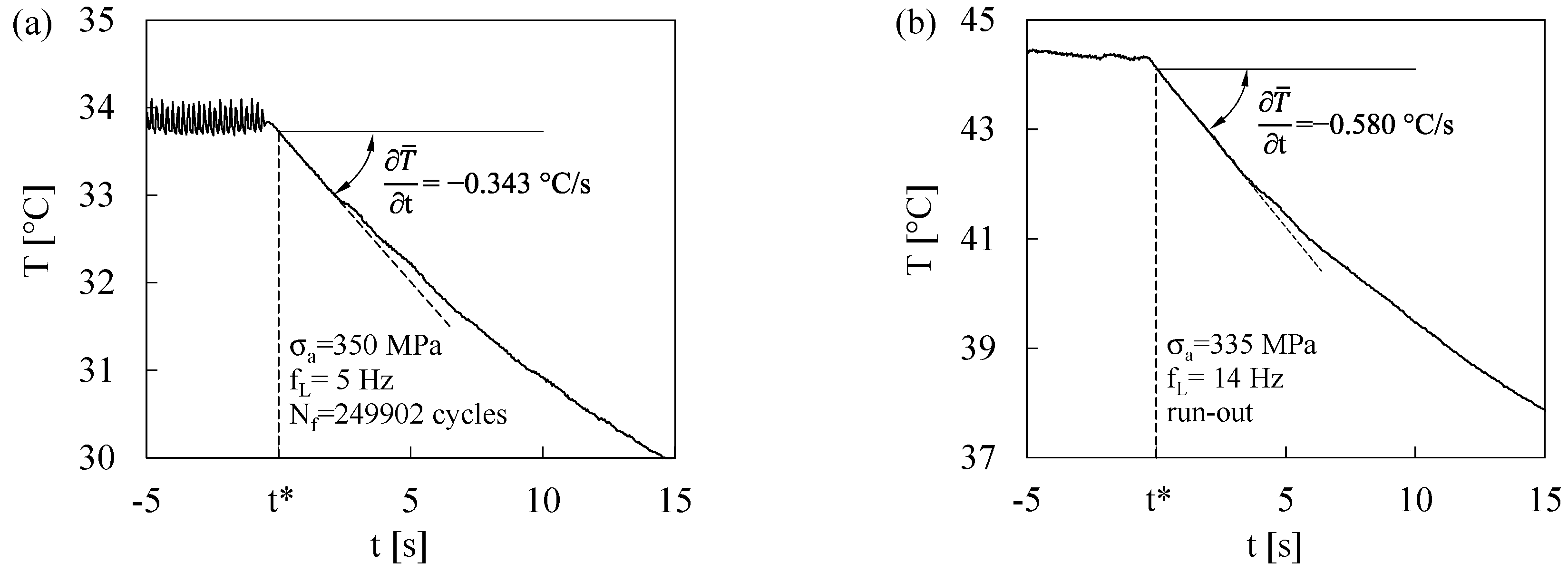
During seven (out of a total of eight) staircase tests, the $\overline{Q}$ parameter was measured, and its evolution was monitored carrying out several test stops during a single fatigue test, according to Equation (7). Typical examples of material cooling gradients are shown in Figure 10a,b for applied stress amplitudes σ_a equal to 350 and 335 MPa, respectively. In both cases, after t = t*, the time window used to calculate the cooling gradient was on the order of some seconds, and the corresponding temperature drop was on the order of 1 °C. Figure 11 shows the evolution of the $\overline{Q}$ parameter versus the number of cycles normalized with respect to 10 millions. It is worth noting that different $\overline{Q}$ trends were observed for the same value of the applied stress amplitude σ_a, depending on the fatigue life experienced by the single specimens. In fact, one can note that slightly decreasing or practically constant $\overline{Q}$ trends were observed in the case of unbroken specimens, spanning the range of 0.123–0.155 MJ/(m³·cycle). Conversely, 1.7 times higher $\overline{Q}$ values were measured in the case of specimens loaded at σ_a = 320 MPa (i.e., below the fatigue limit), which failed at N_f = 982,064 cycles. In the authors’ opinion, this result can be interpreted as a better capability of the $\overline{Q}$ parameter to account for the actual material cyclic evolution with respect to the applied stress amplitude, according to [38].

According to [15,16,18,35,38], the results of staircase fatigue tests were reanalyzed in terms of the characteristic value of the specific heat loss $\overline{Q}$ measured at 50% of the fatigue life. Figure 12 shows that the new fatigue data were well rationalized by the heat energy-based scatter band previously calibrated by the authors in [15].

5. Temperature-Based Approaches

Four step-load fatigue tests were carried out to estimate the material fatigue limit by means of the RM [5]. Figure 13 shows, as an example, the typical material temperature increment measured during the two step-load fatigue tests carried out by imposing f_L = 5 Hz. The relevant ΔT_st values versus the applied stress amplitude for the RM are reported in Figure 14. The same procedure was applied to analyze the data generated from step-load fatigue tests at f_L equal to 1Hz and 10 Hz. Finally, the material fatigue limit was estimated by averaging the fatigue limit evaluated in the step-load fatigue test with individual test frequencies, i.e., ${\mathsf{\sigma }}_{\mathrm{A},\mathrm{RM}}$ = (278 + 286 + 310)/3 = 291 MPa.

Two tensile static tests were carried out for the rapid determination of the fatigue limit according to [8], and the results are shown in Figure 15. The stress corresponding to the end of the temperature linear trend was equal to 293 and 294 MPa for specimens 1 and 2, respectively. Then, the material fatigue limit was evaluated by averaging the results obtained, i.e., ${\mathsf{\sigma }}_{\mathrm{A},\mathrm{static}}=293.5\mathrm{MPa}$.

6. Energy-Based Approaches

The stabilized hysteresis loops measured during the step-load fatigue tests are shown in Figure 16, and the step-load fatigue data reanalyzed in terms of $\overline{W}$ are plotted in Figure 17. To rapidly estimate the fatigue limit, the data were fitted by using two distinct power law regression lines, since it was found that they were characterized by an improved coefficient of correlation (R-squared) as compared to the linear regression. Figure 17 shows that the $\overline{W}$-σ_a data were not characterized by an abrupt change, making the fatigue limit evaluation questionable. To overcome this issue, the regression lines were fitted solely on data clearly below and above the knee point. Afterwards, the fatigue limit was estimated by the intersection of the two regression lines. Finally, the material fatigue limit was estimated by averaging the fatigue limits obtained from the individual step-load fatigue test, i.e., ${\mathsf{\sigma }}_{\mathrm{A},\overline{\mathrm{W}}}$ = (307 + 346 + 340 + 318)/4 = 328 MPa.

During the step-load fatigue tests, the material temperature was monitored by using an infrared camera to evaluate the $\overline{Q}$ parameter according to Equation (7) and to apply the Shiozawa et al. [11,12] approach. Figure 18a,b shows, as an example, the second harmonic of the temperature signal and the succeeding cooling gradient, respectively, observed during a step-load fatigue test, when σ_a = 285 MPa. It can be seen that ΔT_D (see Equation (8)) was equal to 0.006 °C; the temperature drop in the time window adopted to measure the cooling gradient was approximately 0.15 °C. The higher the applied stress amplitude, the higher the ΔT_D and the cooling gradient, as shown in Figure 18c,d, respectively, at σ_a = 345 MPa. It can be seen that ΔT_D (see Equation (8)) was equal to 0.0121 °C, and the temperature drop was approximately 0.3 °C.

Figure 19 shows the $\overline{Q}$ parameter evaluated according to Equation (7) and the fitting lines by using two distinct power law regression lines, since it was again found that they were characterized by a greater coefficient of correlation (R-squared) as compared to the linear regression. Similar to the previous Figure 17, the fatigue limit from individual specimens was estimated by the intersection of the two regression lines. Finally, the material fatigue limit was evaluated by averaging the individual fatigue limits, i.e ${\mathsf{\sigma }}_{\mathrm{A},\overline{\mathrm{Q}}}=\left(316+307+353+348\right)/4=331\mathrm{MPa}$.

Figure 20 shows the results of step-load fatigue tests, reanalyzed according to the Shiozawa et al. approach [12]. The q parameter, calculated according to Equation (10), and the phase difference $\Delta \mathsf{\theta }$, determined according to Equation (12), were plotted against σ_a to evaluate $\Delta \widehat{\mathsf{\theta }}$. For the present material and test conditions, the q versus σ_a trends showed an abrupt change. Following [10], the material fatigue limit was evaluated by averaging the fatigue limit determined in the single-step load fatigue test, i.e., ${\mathsf{\sigma }}_{\mathrm{A},\mathrm{q}}=\left(331+331+361+357\right)/4=345\mathrm{MPa}$. The $\Delta \mathsf{\theta }$ versus σ_a trends were characterized by a high level of scatter, which made the evaluation of $\Delta \widehat{\mathsf{\theta }}$ difficult, mainly in the case of the P_8 and P_9 specimens (see Figure 20). In the authors’ opinion, this was related to the limited number of load steps applied above the fatigue limit, due to specimen failure occurring at σ_a = 365 MPa and σ_a = 345 MPa, respectively.

Despite the scatter observed for $\Delta \mathsf{\theta }$, according to [11,12], the $\Delta \widehat{\mathsf{\theta }}$ value was calculated for each tested specimen, averaging the $\Delta \mathsf{\theta }$ values measured for applied stress amplitudes higher than the fatigue limit. The $\Delta \widehat{\mathsf{\theta }}$ values calculated for each specimen are reported in Figure 20. Knowing $\Delta \widehat{\mathsf{\theta }}$, $\Delta {\widehat{T}}_{\mathrm{D}}$ was calculated according to Equation (15), and then the dissipated energy $\widehat{q}$ was determined by means of Equation (16). Finally, for each tested specimen, the rate of the dissipated energy dq/dσ_a was calculated according to the “conventional lock-in method” and the “phase lock-in method”, by considering two subsequent measurements. Figure 21 shows the dq/dσ_a versus σ_a trends. It can be seen that due to the scatter of the data, the material fatigue limit was estimated considering the results relevant to the P_8 and P_11 specimens (see Figure 20a,d), as ${\mathsf{\sigma }}_{\mathrm{A},\mathrm{dq}/\mathrm{d}{\mathsf{\sigma }}_{\mathrm{a}}}=\left(323+345\right)/2=334\mathrm{MPa}$, and ${\mathsf{\sigma }}_{\mathrm{A},\widehat{\mathrm{q}}}=\left(340+340\right)/2=340\mathrm{MPa}$, according to the “conventional lock-in method” and the “phase lock-in method”, respectively.

Figure 22 shows the comparison among the material fatigue limits evaluated according to the different approaches and that evaluated according to the staircase procedure, represented by the horizontal dashed line. The scatter bands relevant to the temperature—and the energy—based methods were calculated considering the maximum and the minimum values measured for individual specimens. For the staircase result, the 10–90% survival probability scatter band was considered, as shown in Figure 9. The fatigue limits evaluated according to the energy–based methods were close to σ_A,−1, while differences of 11.8% and 11.0% were found by using the Risitano method and the temperature method based on the static tensile test, respectively.

7. Discussion

In the light of the above, the need for one specimen is only virtual: a certain scatter from specimen to specimen exists. To account for this scatter while maintaining the approach fast and simple, the present tests suggest that at least three specimens should be used.

Concerning the approach based on the characteristic phase difference $\Delta \widehat{\mathsf{\theta }}$ [11,12], for the present material and the adopted test conditions, $\Delta \widehat{\mathsf{\theta }}$ measured on one specimen at stress levels greater than the fatigue limit did not stabilize at a characteristic common value but presented a certain scatter; secondly, the scatter bands of $\Delta \widehat{\mathsf{\theta }}$ generated by testing different specimens exhibited different mean values. In the authors’ opinion, this can be related to the limited number of load steps applied above the fatigue limit, due to the specimen failure. This issue might have been solved by adopting smaller load-step increments. These experimental outcomes, as opposed to those reported in other publications [11,12], deserve further assessment in the future.

Note that the regression lines shown in Figure 13, Figure 14, Figure 16, Figure 18, Figure 19 and Figure 20 were defined considering sets of data that were arbitrary chosen by the authors, since in [5,8,11], information on this aspect is incomplete. Moreover, regarding the use of the $\overline{W}$ and/or the $\overline{Q}$ parameters, the definition of a standardized and non-subjective procedure is beyond the scope of the paper. A possible way to overcome this weakness, reducing the uncertainty of the fatigue limit evaluation, is to adopt the iteration procedures proposed in [6,39].

Finally, it is worth noting that all the thermometric approaches are influenced by the uncertainty inherent to the resolution of the thermographic equipment adopted, mainly testing materials that show vanishing temperature increments for applied stress amplitude approaching the fatigue limit. Moreover, regarding the temperature-based approaches, the fatigue limit evaluation is undoubtedly influenced by thermal (room and machine grip temperature) and mechanical (test frequency and specimen geometry) boundary conditions [40].

8. Conclusions

In this paper, different experimental approaches for an engineering evaluation of a material fatigue limit, defined in the Classical High-Cycle Fatigue regime, were analyzed and compared. In particular, the considered approaches were grouped on the basis of the parameter considered as the fatigue damage index. Accordingly, some temperature- and energy-based methods were analyzed. Regarding the temperature-based approaches, the Risitano method and the thermal response in a static tensile test were adopted. As for the energy-based methods, the mechanical ($\overline{W}$ parameter) or the heat ($\overline{Q}$ parameter) energy density per cycle, as well as Shiozawa et co-authors approaches, were analyzed.

The different approaches were applied to evaluate the fatigue limit of a cold-drawn AISI 304L stainless steel in push–pull fatigue tests (R = −1), and it was found that the fatigue limits estimated by using all the analyzed approaches were in agreement, allowing a rapid assessment of the fatigue limit similar to that evaluated by carrying out a short staircase procedure at 10 million cycles. In particular, by using the Risitano method and the thermal response in a static tensile test, a difference of 11.8% and 11.0% was observed, respectively. On the contrary, differences lower than 4% were found by using the energy-based methods. Considering the laboratory facilities, which usually include extensometers or strain gauges, the method based on the $\overline{W}$ parameter seems to be the easiest and most inexpensive to apply among the energy-based methods. If the infrared camera is substituted by temperature sensors like thermocouple wires, also the cooling gradient technique becomes easily affordable. However, the hysteresis energy method remains superior in terms of time saving as compared to the cooling gradient technique, which requires test stops to evaluate $\overline{Q}$. Considering the time required for data processing, the evaluation of the hysteresis energy is faster also compared to the 2nd-harmonic-based approaches.

References

- Dengel, D.; Harig, H. Estimation of the fatigue limit by progressively-increasing load tests. Fatigue Fract. Eng. Mater. Struct. 1980, 3, 113–128. [Google Scholar] [CrossRef]
- Curti, G.; Geraci, A.; Risitano, A. A new method for rapid determination of the fatigue limit. Ing. Automotoristica 1989, 42, 634–636. (In Italian) [Google Scholar]
- Luong, M.P. Infrared thermographic scanning of fatigue in metals. Nuclear Eng. Des. 1995, 158, 363–376. [Google Scholar] [CrossRef] [Green Version]
- Luong, M.P. Fatigue limit evaluation of metals using an infrared thermographic technique. Mech. Mater. 1998, 28, 155–163. [Google Scholar] [CrossRef]
- La Rosa, G.; Risitano, A. Thermographic methodology for rapid determination of the fatigue limit of materials and mechanical components. Int. J. Fatigue 2000, 22, 65–73. [Google Scholar] [CrossRef]
- Curà, F.; Curti, G.; Sesana, R. A new iteration method for the thermographic determination of fatigue limit in steels. Int. J. Fatigue 2005, 27, 453–459. [Google Scholar] [CrossRef]
- De Finis, R.; Palumbo, D.; Ancona, F.; Galietti, U. Fatigue limit evaluation of various martensitic stainless steels with new robust thermographic data analysis. Int. J. Fatigue 2015, 74, 88–96. [Google Scholar] [CrossRef]
- Risitano, A.; Risitano, G. Determining fatigue limits with thermal analysis of static traction tests. Fatigue Fract. Eng. Mater. Struct. 2013, 36, 631–639. [Google Scholar] [CrossRef]
- Krapez, J.C.; Pacou, D.; Gardette, G. Lock-in thermography and fatigue limit of metals. In Proceedings of the Q.I.R.T, Reims, France, 18–21 July 2000. [Google Scholar]
- Akai, A.; Shiozawa, D.; Sakagami, T. Fatigue limit evaluation for austenitic stainless steel. J. Soc. Mat. Sci. Jpn. 2012, 61, 953–959. [Google Scholar] [CrossRef]
- Shiozawa, D.; Inagawa, T.; Akai, A.; Sakagami, T. Accuracy improvement of dissipated energy measurement and fatigue limit estimation by using phase information. In Proceedings of the AITA workshop, Pisa, Italy, 29 September–2 October 2015. [Google Scholar]
- Shiozawa, D.; Inagawa, T.; Washio, T.; Sakagami, T. Fatigue limit estimation of stainless steel with new dissipated energy data analysis. Procedia Struct. Integr. 2016, 2, 2091–2096. [Google Scholar] [CrossRef]
- Palumbo, D.; Galietti, U. Thermoelastic Phase Analysis (TPA): A new method for fatigue behaviour analysis of steel. Fatigue Fract. Eng. Mater. Struct. 2017, 40, 523–534. [Google Scholar] [CrossRef]
- Meneghetti, G. Analysis of the fatigue strength of a stainless steel based on the energy dissipation. Int. J. Fatigue 2007, 29, 81–94. [Google Scholar] [CrossRef]
- Meneghetti, G.; Ricotta, M.; Atzori, B. A synthesis of the push-pull fatigue behaviour of plain and notched stainless steel specimens by using the specific heat. Fatigue Fract. Engng. Mater. Struct. 2013, 36, 1306–1322. [Google Scholar] [CrossRef]
- Meneghetti, G.; Ricotta, M. The use of the specific heat loss to analyse the low- and high cycle fatigue behaviour of plain and notched specimens made of a stainless steel. Eng. Fract. Mech. 2012, 81, 2–16. [Google Scholar] [CrossRef]
- Meneghetti, G.; Ricotta, M.; Atzori, B. The heat energy dissipated in a control volume to correlate the fatigue strength of bluntly and severely notched stainless steel specimens. In Proceedings of the 21st European Conference on Fracture, ECF21, Catania, Italy, 20–24 June 2016; pp. 2076–2083. [Google Scholar]
- Rigon, D.; Ricotta, M.; Meneghetti, G. An analysis of the specific heat loss at the tip of severely notched stainless steel specimens to correlate the fatigue strength. Theor. Appl. Fract. Mech. 2017, 92, 240–251. [Google Scholar] [CrossRef]
- Meneghetti, G.; Ricotta, M.; Negrisolo, L.; Atzori, B. A synthesis f the fatigue behaviour of stainless steel bars under fully reversed axial or torsion loading by using the specific heat loss. Key Eng. Mater. 2013, 577–578, 453–456. [Google Scholar] [CrossRef]
- Ellyin, F. Fatigue Damage, Crack Growth and Life Prediction; Chapman & Hall: London, UK, 1997. [Google Scholar]
- Dixon, W.J.; Mood, A.M. A method for obtaining and analyzing sensitivity data. J. Am. Stat. Assoc. 1948, 43, 109–126. [Google Scholar] [CrossRef]
- Constantinescu, A.; Dang Van, K.; Maitournam, M.H. A unified approach for high and low cycle fatigue based on shakedown concepts. Fatigue Fract. Eng. Mater. Struct. 2003, 26, 561–568. [Google Scholar] [CrossRef]
- Wong, A.K.; Kirby, G.C. A hybrid numerical/experimental technique for determining the heat dissipated during low cycle fatigue. Eng. Fract. Mech. 1990, 37, 493–504. [Google Scholar] [CrossRef]
- Germain, P.; Nguyen, Q.S.; Suquet, P. Continuum Thermodynamics. Trans. ASME J. Appl. Mech. 1983, 50, 1010–1020. [Google Scholar] [CrossRef]
- Lemaitre, J.; Chaboche, J.L. Mechanics of Solid Materials; Cambridge University Press: Cambridge, UK, 1998. [Google Scholar]
- Chrysochoos, A.; Louche, H. An Infrared image process to analyse the calorific effects accompanying strain localization. Int. J. Eng. Sci. 2000, 38, 1759–1788. [Google Scholar] [CrossRef]
- Rousselier, G. Dissipation in porous metal plasticity and ductile fracture. J. Mech. Phys. Solids 2001, 49, 1727–1746. [Google Scholar] [CrossRef]
- Chrysochoos, A.; Berthel, B.; Latourte, F.; Galtier, A.; Pagano, S.; Watrisse, B. Local energy analysis of high cycle fatigue using digital image correlation and infrared thermography. J. Strain. Anal. 2008, 43, 411–421. [Google Scholar] [CrossRef]
- Meneghetti, G.; Ricotta, M. The heat energy dissipated in the material structural volume to correlate the fatigue crack growth rate in stainless steel specimens. Int. J. Fatigue 2018, 115, 107–119. [Google Scholar] [CrossRef]
- Pandey, K.N.; Chand, S. Deformation based temperature rise: A review. Int. J. Pres. Ves. Pip. 2003, 80, 673–687. [Google Scholar] [CrossRef]
- Charkaluk, E.; Constantinescu, A. Dissipation and fatigue damage. In Proceedings of the Fifth International Conference on Low Cycle Fatigue LCF 5, Berlin, Germany, 9–11 September 2003. [Google Scholar]
- Plekhov, O.A.; Panteleev, I.A.; Naimark, O.B. Energy accumulation and dissipation in metals as a result of structural-scaling transitions in a mesodefect ensemble. Phys. Mesomech. 2007, 10, 294–301. [Google Scholar] [CrossRef]
- Feltner, C.E.; Morrow, J.D. Microplastic strain hysteresis energy as a criterion for fatigue fracture. Trans. ASME Series D J. Basic Eng. 1961, 83, 15–22. [Google Scholar] [CrossRef]
- Halford, G.R. The energy required for fatigue. J. Mat. 1966, 1, 3–18. [Google Scholar]
- Meneghetti, G.; Ricotta, M.; Atzori, B. A two-parameter, heat energy-based approach to analyse the mean stress influence on axial fatigue behaviour of plain steel specimens. Int. J. Fatigue 2016, 82, 60–70. [Google Scholar] [CrossRef]
- Fan, J.; Zhao, Y.; Guo, X. A unifying energy approach for high cycle fatigue behavior evaluation. Mech. Mater. 2018, 120, 15–25. [Google Scholar] [CrossRef]
- Jang, J.Y.; Khonsari, M.M. On the evaluation of fracture fatigue entropy. Theor. Appl. Fract. Mech. 2018, 96, 351–361. [Google Scholar] [CrossRef]
- Meneghetti, G.; Ricotta, M.; Atzori, B. Experimental evaluation of fatigue damage in two-stage loading tests based on the energy dissipation. Pro. Inst. Mech. Eng. Part C Mech. Eng. Scie 2015, 229, 1280–1291. [Google Scholar] [CrossRef]
- Huang, J.; Pastor, M.A.; Garnier, C.; Xiaojing Gong, X. Rapid evaluation of fatigue limit on thermographic data analysis. Int. J. Fatigue 2017, 104, 293–301. [Google Scholar] [CrossRef] [Green Version]
- Fernzandez-Canteli, A.; Castillo, E.; Argüelles, A.; Fernandez, P.; Canales, M. Checking the fatigue limit from thermographic techniques by means of a probabilistic model of the epsilon-N field. Int. J. Fatigue 2012, 39, 109–115. [Google Scholar] [CrossRef]
Figure 1.
(a) Energy balance for a material undergoing fatigue loadings and (b) evolution of the average temperature per cycle.
Figure 2.
Material temperature evolution during a constant amplitude fatigue test (a); material fatigue limit evaluation according to the Risitano method [5] (b).
Figure 3.
Temperature-versus-stress curve measured during a tensile static test and material fatigue limit evaluation according to [8].
Figure 4.
Temperature evolution starting from the beginning of a fatigue test and evaluation of the cooling gradient after stationary conditions are achieved.
Figure 5.
Rapid material fatigue limit evaluation assuming (a) the input mechanical energy per cycle and (b) the dissipated thermal energy per cycle as fatigue damage indexes.
Figure 6.
First and second harmonic of the temperature signal measured during a fatigue test.
Figure 7.
Rapid material fatigue limit evaluation according to the “phase lock-in method” [12].
Figure 8.
Specimen geometry for (a) staircase fatigue tests and (b) static- and step-load fatigue tests.
Figure 9.
Push-pull, stress-life curve of AISI 304L cold-drawn bars.
Figure 10.
Typical cooling gradients measured during the staircase fatigue tests: (a) σa = 350 MPa, fL = 5 Hz, Nf = 249,902 cycles; (b) σa = 335 MPa, fL = 14 Hz, run-out.
Figure 11.
trends vs. the number of cycles normalized with respect to 10 million.
Figure 12.
Comparison of the present staircase fatigue test results and the -based fatigue curve (from [35]).
Figure 13.
Example of temperature evolution measured during step-load fatigue tests carried out to estimate the material fatigue limit according to the Risitano method [5].
Figure 14.
Risitano method [5] applied to AISI 304L cold-drawn bars.
Figure 15.
Material temperature evolution during the tensile static test on specimen 1 (a) and specimen 2 (b).
Figure 16.
Stabilized hysteresis loops measured during the step-load fatigue tests for (a) P_9, (b) P_10, (c) P_11 and (d) P_12 specimens.
Figure 17.
Step-load fatigue tests reanalyzed in terms of for (a) P_9, (b) P_10, (c) P_11 and (d) P_12 specimens.
Figure 18.
Example of (a,c) second harmonic of temperature signal and (b,d) cooling gradient during step-load tests at (a,b) σa = 285 MPa and (c,d) σa = 345 MPa.
Figure 19.
Step load-fatigue tests reanalyzed in terms of the parameter, calculated according to Equation (7) for (a) P_7, (b) P_9, (c) P_10 and (d) P_11 specimens.
Figure 20.
Step load-fatigue tests reanalyzed in terms of the q parameter (Equation (10)) and phase difference (Equation (12)) for (a) P_8, (b) P_9, (c) P_10, and (d) P_11 specimens.
Figure 21.
Step load-fatigue tests reanalyzed in terms of the rate of the parameter according to the “phase lock-in method” and in terms of the rate of the q parameter, according to the “conventional lock-in method”, for (a) P_8, (b) P_9, (c) P_10, and (d) P_11 specimens.
Figure 22.
Comparison among the fatigue limits σA,−1 calculated according to different experimental approaches.