
Exploring the Optimal Scale of Coastal Reclamation Activities Based on an Environmental Capacity Assessment System: A Case Study in Haizhou Bay, China
Abstract
:1. Introduction
2. Materials and Methods
2.1. Study Area and Data
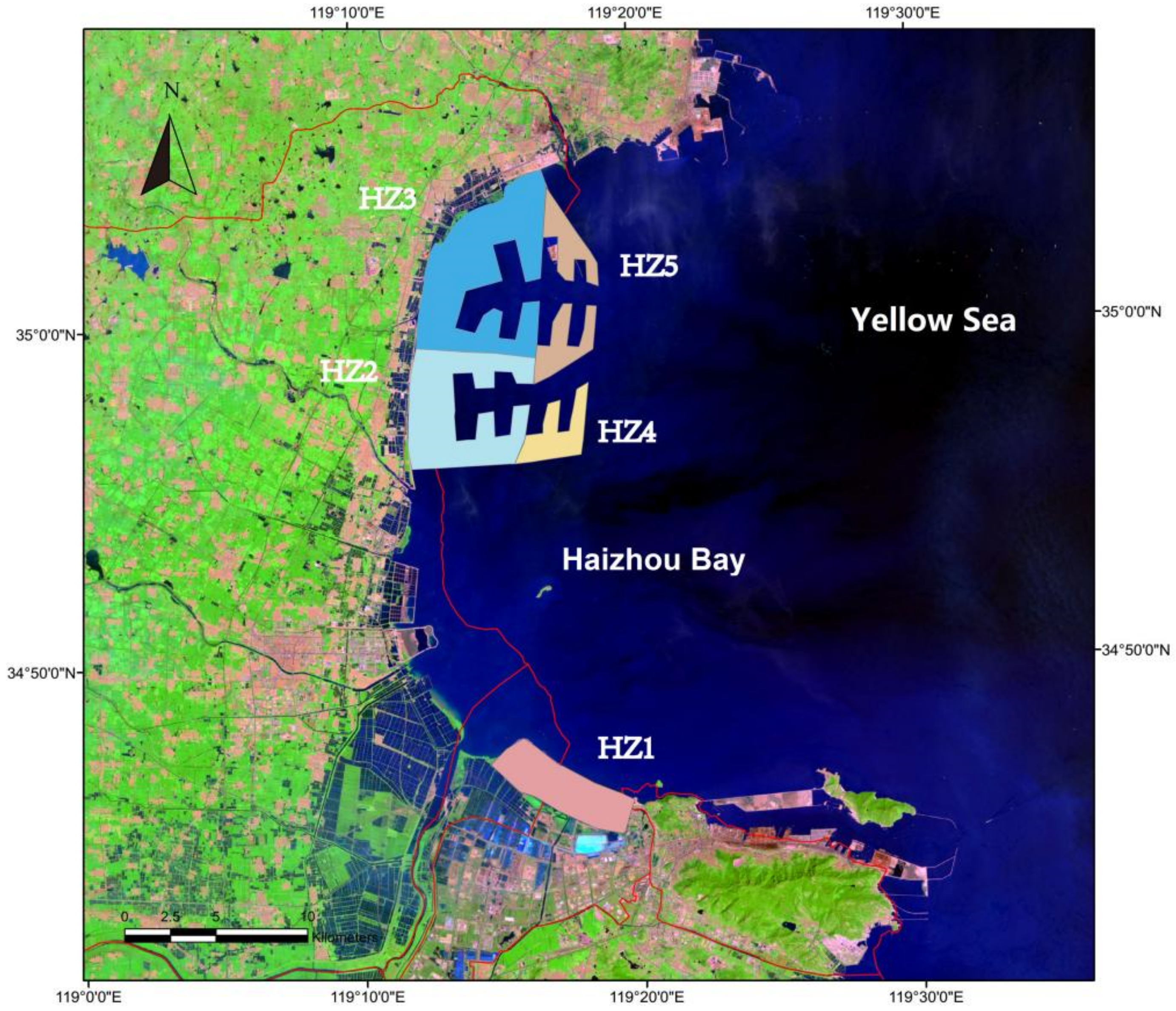
2.1.1. Study Area
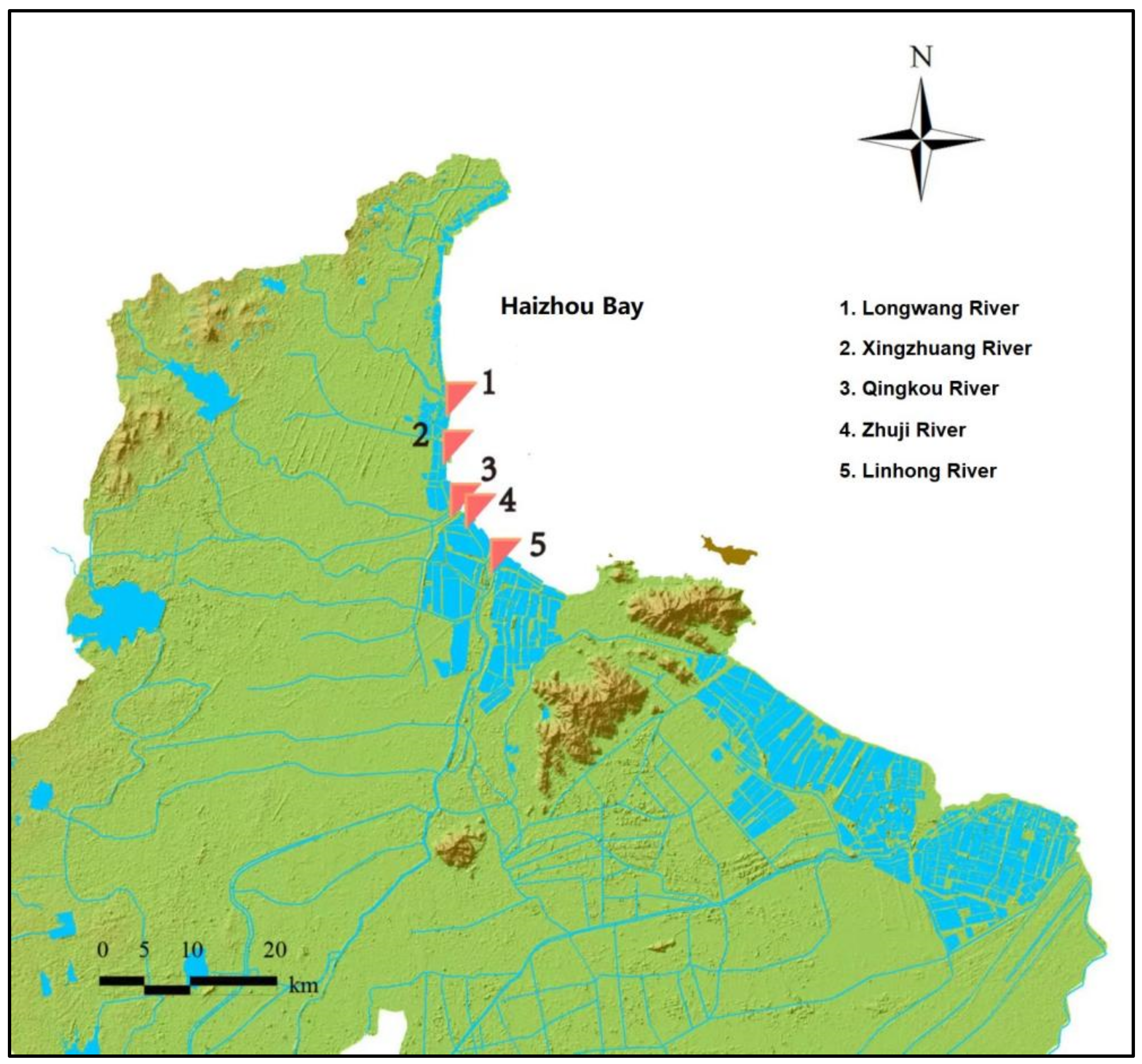
2.1.2. Study Data
(1) Major Sewage Outfalls
(2) Main Rivers
2.2. Environmental Capacity Assessment System (ECAS)
2.2.1. Environmental Capacity Theory
2.2.2. Environmental Capacity Assessment Indicators
2.2.3. Environmental Capacity Estimation
Hydrodynamic Model
- 1.
- Basic hydrodynamic model.
- : time;
- : acceleration of gravity ;
- : free water level (m);
- : depth of the water (m), the distance from the bottom of the sea to the stationary sea surface;
- : flow density in the direction, that is, the width of the flow ;
- : directional perpendicular mean velocity component;
- : the coefficient of Chezy, its relation to the Manning number M is ;
- : wind friction factor ; is the wind stress coefficient, is the air density;
- : wind speed, and component of wind speed in direction ;
- : Coriolis coefficient , is the rotational speed of the earth, is geographic latitude.
- 2.
- Boundary conditions.
Water Quality Model
- 1.
- Basic water quality model.
- h: depth of the water (m);
- c: concentration of pollutant (any unit);
- x, y: horizontal velocity component in the x and y directions (m/s);
- Dx, Dy: dispersion in the x and y directions (m2/s);
- F: linear attenuation coefficient (seconds −1);
- S:Qs (cs-c);
- Qs: source and sink;
- Cs: pollutant emission concentrations in sources and sinks. The flow velocity and other information (including u, v and h) at each time step are provided by the hydrodynamic module.
- 2.
- The boundary conditions.
- 3.
- Related parameters.
Linear Programming Model
- Z: objective function;
- Q: coefficient vector; when the total amount of pollutants reaches the maximum value, Q = [1, 1,…, 1]T;
- A: response coefficient matrix, generated by the concentration response field of pollution sources and the water quality monitoring points;
- : pollution contribution coefficient of unit load of the jth sewage outlet to the ith water quality monitoring point;
- m: number of water quality monitoring points;
- n: number of pollution sources;
- B: pollutant background concentration vector, ;
- S: standard vector of water quality, ;
- X: pollutants discharge load, ; : the lower limit vector of pollutant discharge load, ; : the upper limit vector of pollutant discharge load, ;
Determination of Water Quality Objectives
Response Coefficient Field
2.2.4. Comprehensive Assessment
3. Results and Discussion
3.1. Scenario 1 (S1)
3.1.1. Calculation Area of EC
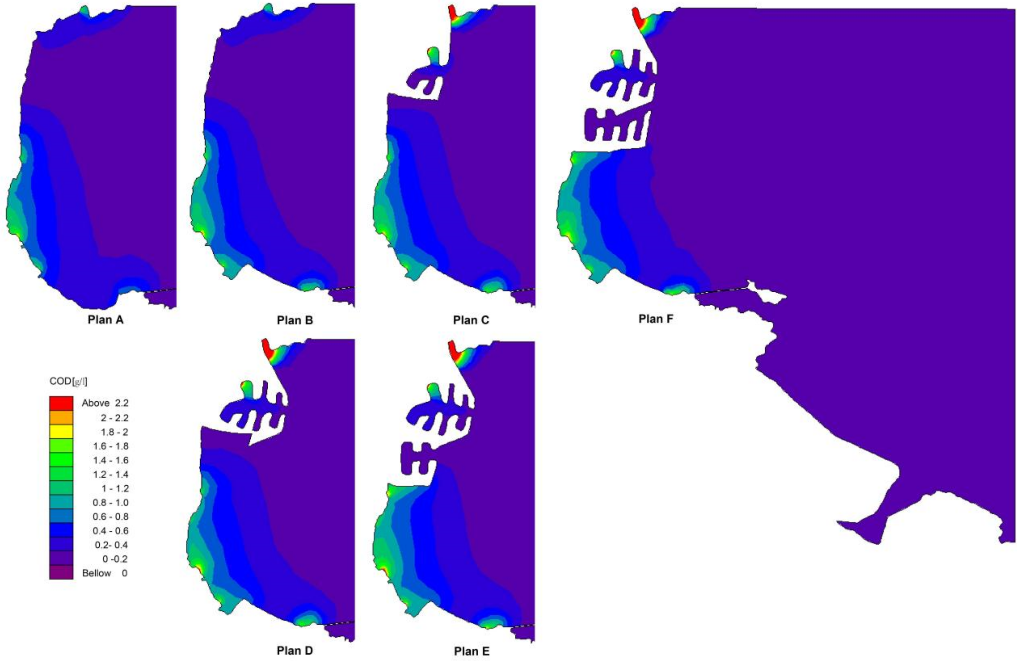
3.1.2. COD
3.1.3. NH4-N
3.1.4. NOX-N
3.1.5. PO4-P
3.1.6. Comprehensive Evaluation of Feasibility
3.2. Scenario 2 (S2)
3.2.1. Calculation area of EC
3.2.2. COD
3.2.3. NH4-N
3.2.4. NOX-N
3.2.5. PO4-P
3.2.6. Comprehensive Evaluation of Feasibility
3.3. Scenario 3 (S3)
3.3.1. Calculation Area of EC
3.3.2. COD
3.3.3. NH4-N
3.3.4. NOX-N
3.3.5. PO4-P
3.3.6. Comprehensive Evaluation of Feasibility
3.4. Comprehensive Analysis
4. Conclusions
Supplementary Materials
Author Contributions
Funding
Institutional Review Board Statement
Informed Consent Statement
Data Availability Statement
Conflicts of Interest
References
- Kennedy, V.S.; Twilley, R.R.; Kleypas, J.A.; Cowan, J.H.J.; Hare, S.R. Coastal and Marine Ecosystems & Global Climate Change: Potential Effects on U.S., Resources; Pew Center on Global Climate Change: Arlington, VA, USA, 2002. [Google Scholar]
- Lin, L.; Pussella, P. Assessment of vulnerability for coastal erosion with GIS and AHP techniques case study: Southern coastline of Sri Lanka. Nat. Resour. Model. 2017, 30, e12146. [Google Scholar] [CrossRef]
- Wessells, A.T. Urban Blue Space and “The Project of the Century”: Doing Justice on the Seattle Waterfront and for Local Residents. Buildings 2014, 4, 764–784. [Google Scholar] [CrossRef] [Green Version]
- State Oceanic Administration (SOA). Bulletin of China’s Marine Economy 2019. Beijing, China. 2020. Available online: http://www.nmdis.org.cn/hygb/zghyjjtjgb/2019hyjjtjgb/ (accessed on 20 May 2020).
- Ren, C.; Wang, Z.; Zhang, Y.; Zhang, B.; Chen, L.; Xi, Y.; Xiao, X.; Doughty, R.B.; Liu, M.; Jia, M.; et al. Rapid expansion of coastal aquaculture ponds in China from Landsat observations during 1984–2016. Int. J. Appl. Earth Obs. Geoinf. 2019, 82, 101902. [Google Scholar] [CrossRef]
- Neumann, B.; Vafeidis, A.T.; Zimmermann, J.; Nicholls, R.J. Future Coastal Population Growth and Exposure to Sea-Level Rise and Coastal Flooding—A Global Assessment. PLoS ONE 2015, 10, e0118571. [Google Scholar] [CrossRef] [PubMed] [Green Version]
- Feng, L.H.; Ma, Y.J. Evolution of tidal flats in China and ecological exploitation of tidal flat resources. Environ. Earth Sci. 2012, 67, 1639–1649. [Google Scholar] [CrossRef]
- Wang, W.; Liu, H.; Li, Y.; Su, J. Development and management of land reclamation in China. Ocean Coast. Manag. 2014, 102, 415–425. [Google Scholar] [CrossRef]
- Muller, J.R.M.; Chen, Y.; Aarninkhof, S.G.J.; Chan, Y.-C.; Piersma, T.; van Maren, D.S.; Tao, J.; Wang, Z.B.; Gong, Z. Ecological impact of land reclamation on Jiangsu coast (China): A novel ecotope assessment Tongzhou Bay. Water Sci. Eng. 2020, 13, 57–64. [Google Scholar] [CrossRef]
- Ren, C.; Wang, Z.; Zhang, B.; Li, L.; Chen, L.; Song, K.; Jia, M. Remote Monitoring of Expansion of Aquaculture Ponds Along Coastal Region of the Yellow River Delta from 1983 to 2015. Chin. Geogr. Sci. 2018, 28, 430–442. [Google Scholar] [CrossRef] [Green Version]
- Zhang, Y.; Chen, R.; Wang, Y. Tendency of land reclamation in coastal areas of Shanghai from 1998 to 2015. Land Use Policy 2020, 91, 104370. [Google Scholar] [CrossRef]
- Johnson, J.M.; Moore, L.J.; Ells, K.; Murray, A.B.; Adams, P.N.; MacKenzie, R.A.; Jaeger, J.M. Recent shifts in coastline change and shoreline stabilization linked to storm climate change. Earth Surf. Process. Landf. 2015, 40, 569–585. [Google Scholar] [CrossRef]
- Cui, P.; Ju, X.; Liu, Y.; Li, D. Predicting and Improving the Waterlogging Resilience of Urban Communities in China—A Case Study of Nanjing. Buildings 2022, 12, 901. [Google Scholar] [CrossRef]
- Tian, B.; Wu, W.; Yang, Z.; Zhou, Y. Drivers, trends, and potential impacts of long-term coastal reclamation in China from 1985 to 2010. Estuar. Coast Shelf Sci. 2016, 170, 83–90. [Google Scholar] [CrossRef]
- Xu, N.; Gao, Z.; Ning, J. Analysis of the characteristics and causes of coastline variation in the Bohai Rim (1980–2010). Environ. Earth Sci. 2016, 75, 719. [Google Scholar] [CrossRef]
- Wu, W.; Yang, Z.; Tian, B.; Huang, Y.; Zhou, Y.; Zhang, T. Impacts of coastal reclamation on wetlands: Loss, resilience, and sustainable management. Estuar. Coast. Shelf Sci. 2018, 210, 153–161. [Google Scholar] [CrossRef]
- Ma, T.; Li, X.; Bai, J.; Cui, B. Impacts of coastal reclamation on natural wetlands in large river deltas in China. Chin. Geogr. Sci. 2019, 29, 640–651. [Google Scholar] [CrossRef] [Green Version]
- He, Q.; Bertness, M.D.; Bruno, J.F.; Li, B.; Chen, G.; Coverdale, T.C.; Altieri, A.H.; Bai, J.; Sun, T.; Pennings, S.C.; et al. Economic development and coastal ecosystem change in China. Sci. Rep. 2014, 4, 5995. [Google Scholar] [CrossRef] [Green Version]
- Ma, T.; Li, X.; Bai, J.; Cui, B. Habitat modification in relation to coastal reclamation and its impacts on waterbirds along China’s coast. Glob. Ecol. Conserv. 2019, 17, e00585. [Google Scholar] [CrossRef]
- Murray, N.J.; Phinn, S.R.; DeWitt, M.; Ferrari, R.; Johnston, R.; Lyons, M.B.; Clinton, N.; Thau, D.; Fuller, R.A. The global distribution and trajectory of tidal flats. Nature 2019, 565, 222–225. [Google Scholar] [CrossRef]
- Lin, W.; Xu, D.; Guo, P.; Wang, D.; Li, L.; Gao, J. Exploring variations of ecosystem service value in Hangzhou Bay Wetland, Eastern China. Ecosyst. Serv. 2019, 37, 100944. [Google Scholar] [CrossRef]
- Sengupta, D.; Chen, R.; Meadows, M.E. Building beyond land: An overview of coastal land reclamation in 16 global megacities. Appl. Geogr. 2018, 90, 229–238. [Google Scholar] [CrossRef]
- Yang, H.; Ma, M.; Thompson, J.R.; Flower, R.J. Protect coastal wetlands in China to save endangered migratory birds. Proc. Natl. Acad. Sci. USA 2017, 114, E5491. [Google Scholar] [CrossRef] [PubMed] [Green Version]
- Peng, B.R.; Lin, C.; Jin, D.; Rao, H.H.; Jiang, Y.W.; Liu, Y. Modeling the total allowable area for coastal reclamation: A case study of Xiamen, China. Ocean. Coast. Manag. 2013, 76, 38–44. [Google Scholar] [CrossRef]
- Qiu, L.F.; Zhang, M.; Zhou, B.B.; Cui, Y.Z.; Yu, Z.L.; Liu, T.; Wu, S.H. Economic and ecological trade-offs of coastal reclamation in the Hangzhou Bay, China. Ecol. Indic. 2021, 125, 107477. [Google Scholar] [CrossRef]
- State Oceanic Administration (SOA). Some Suggestion on Strengthen Managment Sea Region Agriculture Reclamation. Beijing, China. 2012. Available online: http://gc.mnr.gov.cn/201806/t20180615_1796980.html/ (accessed on 6 September 2012).
- Li, F.; Ding, D.; Chen, Z.; Chen, H.; Shen, T.; Wu, Q.; Zhang, C. Change of sea reclamation and the sea-use management policy system in China. Mar. Policy 2020, 115, 103861. [Google Scholar] [CrossRef]
- Task Force of the China Council for International Cooperation on Environment and Development (CCICED). Ecosystem Issues and Policy Options Addressing the Sustainable Development of China’s Ocean and Coast; China Environmental Science Press: Beijing, China, 2012. [Google Scholar]
- Xu, N.; Wang, Y.Q.; Huang, C.H.; Jiang, S.; Jia, M.M.; Ma, Y. Monitoring coastal reclamation changes across Jiangsu Province during 1984–2019 using landsat data. Mar. Policy 2022, 136, 104887. [Google Scholar] [CrossRef]
- Wang, Y.B.; Zhang, J.J.; Wu, W.T.; Liu, J.; Ran, X.B.; Zhang, A.J.; Zang, J.Y. Variations in the marine seawater environment and the dominant factors in the Lianyungang coastal area. Reg. Stud. Mar. Sci. 2022, 52, 102276. [Google Scholar] [CrossRef]
- Sun, X.; Li, Y.F.; Zhu, X.D.; Cao, K.; Feng, L. Integrative assessment and management implications on ecosystem services loss of coastal wetlands due to reclamation. J. Clean. Prod. 2017, 163, S101–S112. [Google Scholar] [CrossRef]
- Feng, L.; He, J.; Ai, J.Y.; Sun, X.; Bian, F.Y.; Zhu, X.D. Evaluation for coastal reclamation feasibility using a comprehensive hydrodynamic framework: A case study in Haizhou Bay. Mar. Pollut. Bull. 2015, 100, 182–190. [Google Scholar] [CrossRef]
- Feng, L.; Zhu, X.D.; Sun, X. Assessing coastal reclamation suitability based on a fuzzy-AHP comprehensive evaluation framework: A case study of Lianyungang, China. Mar. Pollut. Bull. 2014, 89, 102–111. [Google Scholar] [CrossRef]
- Yu, W.W.; Zou, X.Q.; Zhang, D.J.; Wang, T.; Wang, C.L.; Yao, Y.L.; Zhang, H.; Ben, C.K.; Yuan, J.M. The evaluation of marine biological value of the Jiangsu coastal zone (east of China) under the interference of human activities. Ecol. Indic. 2019, 102, 76–83. [Google Scholar] [CrossRef]
- Liu, L.; Xu, W.; Yue, Q.; Teng, X.; Hu, H. Problems and countermeasures of coastline protection and utilization in China. Ocean. Coast. Manag. 2018, 153, 124–130. [Google Scholar] [CrossRef]
- GESAMP (Joint Group of Experts on the Scientific Aspects of Marine Pollution). Environmental Capacity, an Approach to Marine Pollution Prevention; GESAMP Reports and Studies No. 30; GESAMP: London, UK, 1986. [Google Scholar]
- Deng, Y.X.; Zheng, B.H.; Fu, G. Study on the total water pollutant load allocation in the Changjiang (Yangtze River) Estuary and adjacent seawater area. Estuarine. Coast. Shelf Sci. 2010, 86, 331–336. [Google Scholar] [CrossRef]
- DHI. Hydrodynamic Module Scientific Documentation. 2021.MIKE 21 & MIKE 3 Flow Model FM—Hydrodynamic and Transport Module. Available online: mikepoweredbydhi.help (accessed on 10 October 2017).
- USEPA. Protocol for Developing Nutrient TMDLs; USEPA Office of Water: Washington, DC, USA, 1999. [Google Scholar]
- Chadderton, R.A.; Kroop, I.S. An Evaluation of eight waste-load allocation methods. Water Resour. Bull. 1985, 21, 833–839. [Google Scholar] [CrossRef]
- Meng, W.; Liu, Z.T.; Zhang, N.; Hu, L.L. The Study on Technique of Basin Water Quality Target Management II: Water Environmental Criteria, Standard and Total Amount Control. Res. Environ. Sci. 2008, 21, 1–8. [Google Scholar]


| Working Condition | Area/km2 | Usage | Reclamation Period |
|---|---|---|---|
| HZ1 | 18 | Urban development | 2010–2015 |
| HZ2 | 22 | Port construction | 2015–2030 |
| HZ3 | 46 | Port construction | 2015–2030 |
| HZ4 | 9 | Port construction | 2015–2030 |
| HZ5 | 19 | Port construction | 2015–2030 |
| Water Quality Monitoring Point | Function Description | Water Quality Standard |
|---|---|---|
| 1 | Storm surge area | Class II |
| 2 | Reserved tourist area | Class Ⅲ |
| 3 | Marine fishing area | Class II |
| 4 | No fishing area | Class II |
| 5 | Sewage discharge area | Class Ⅳ |
| 6 | Mariculture area | Class II |
| 7 | Mariculture area | Class II |
| 8 | Haizhou Bay Tourist Resort | Class Ⅲ |
| 9 | Lianyungang Port area | Class Ⅳ |
| 10 | Coastal salt farming area | Class II |
| 11 | Lianyungang Port area | Class Ⅳ |
| 12 | Fishery breeding area | Class II |
| 13 | Storm surge area | Class Ⅳ |
| Index | Standard | Evaluation Score | Feasibility |
|---|---|---|---|
| (t/a) | ≤4 | 10 | R = average{R1, R2, R3, R4} R ≥ 8, feasible 8 > R ≥ 4, basically feasible R < 4, infeasible |
| ≤8 | 8 | ||
| ≤10 | 4 | ||
| (t/a) | ≤4 | 10 | |
| ≤8 | 8 | ||
| ≤10 | 4 | ||
| (t/a) | ≤4 | 10 | |
| ≤8 | 8 | ||
| ≤10 | 4 | ||
| (t/a) | ≤4 | 10 | |
| ≤8 | 8 | ||
| ≤10 | 4 |
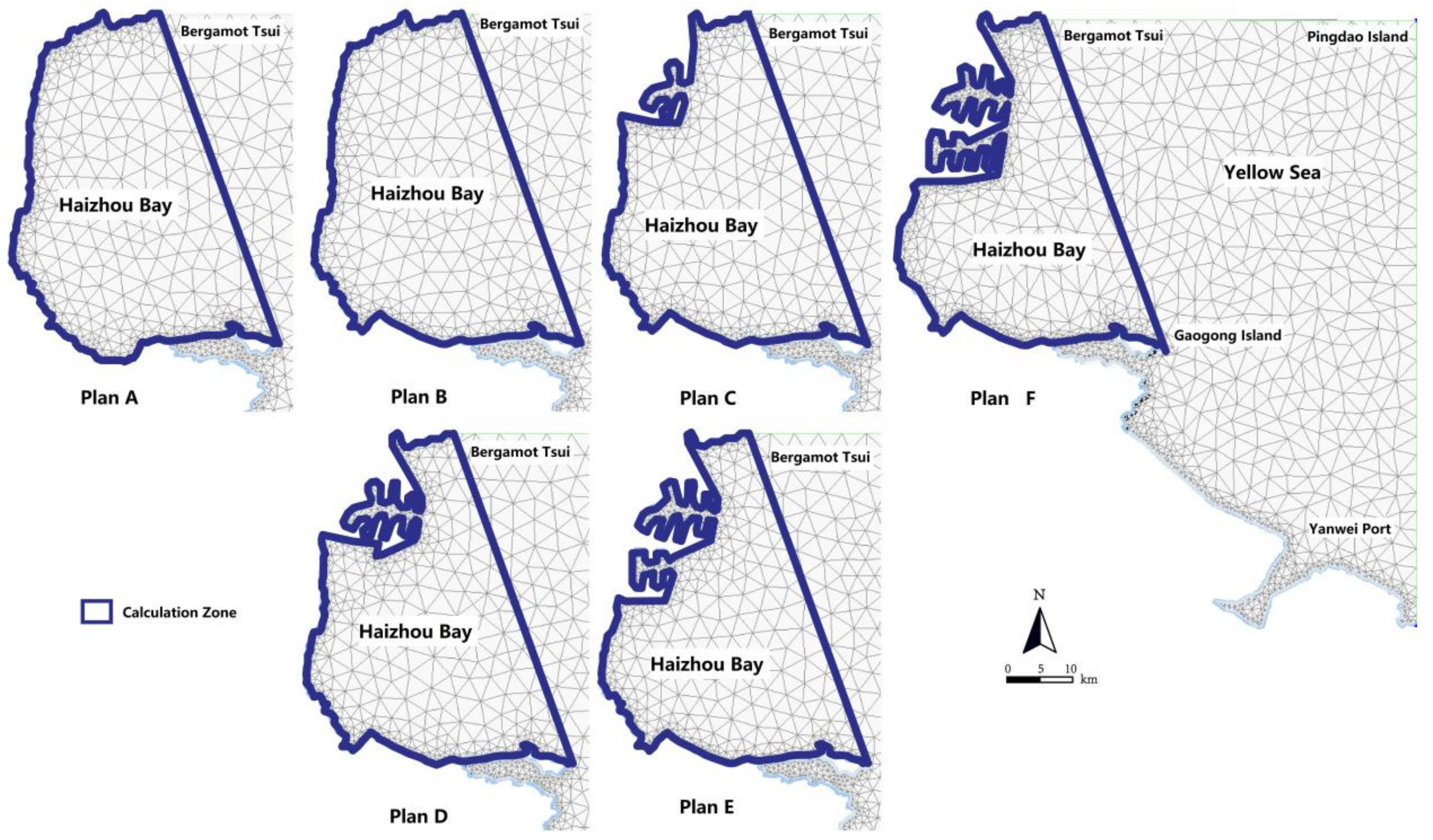
| Reclamation Scheme | Working Conditions | Reclamation Area/km2 | Calculation Area of EC/km2 |
|---|---|---|---|
| A | Current situation (no working condition) | 0.00 | 876.39 |
| B | HZ1 | 18 | 858.39 |
| C | HZ1+HZ2 | 40 | 836.39 |
| D | HZ1+HZ2+HZ3 | 86 | 790.39 |
| E | HZ1+HZ2+HZ3+HZ4 | 95 | 781.39 |
| F | HZ1+HZ2+HZ3+HZ4+HZ5 | 114 | 762.39 |
| Reclamation Scheme | COD (t/a) | EC Change (%) | R1 |
|---|---|---|---|
| A | 62,444 | - | - |
| B | 61,517 | 1.48 | 10 |
| C | 49,213 | 21.19 | 0 |
| D | 47,803 | 23.44 | 0 |
| E | 49,657 | 20.48 | 0 |
| F | 52,314 | 16.22 | 0 |
| Reclamation Scheme | NH4-N(t/a) | EC Change (%) | R2 |
|---|---|---|---|
| A | 3366 | - | - |
| B | 3217 | 4.45 | 8 |
| C | 2645 | 21.43 | 0 |
| D | 2564 | 23.83 | 0 |
| E | 2664 | 20.87 | 0 |
| F | 2831 | 15.90 | 0 |
| Reclamation Scheme | NOX-N(t/a) | EC Change (%) | R3 |
|---|---|---|---|
| A | 5082 | - | - |
| B | 4887 | 3.84 | 10 |
| C | 4139 | 18.56 | 0 |
| D | 3855 | 24.12 | 0 |
| E | 3792 | 25.38 | 0 |
| F | 4021 | 20.88 | 0 |
| Reclamation Scheme | PO4-P(t/a) | EC Change (%) | R4 |
|---|---|---|---|
| A | 421 | - | - |
| B | 410 | 2.58 | 10 |
| C | 373 | 11.49 | 0 |
| D | 321 | 23.87 | 0 |
| E | 345 | 18.16 | 0 |
| F | 332 | 21.11 | 0 |
| Reclamation Scheme | R1 | R2 | R3 | R4 | R | Evaluation Result |
|---|---|---|---|---|---|---|
| A | - | - | - | - | - | - |
| B | 10 | 8 | 10 | 10 | 9.5 | feasible |
| C | 0 | 0 | 0 | 0 | 0 | infeasible |
| D | 0 | 0 | 0 | 0 | 0 | infeasible |
| E | 0 | 0 | 0 | 0 | 0 | infeasible |
| F | 0 | 0 | 0 | 0 | 0 | infeasible |
| Reclamation Scheme | Evaluation Result | Area (km2) | Appropriate Scale of Reclamation (km2) |
|---|---|---|---|
| A | - | 0.00 | 18 |
| B | feasible | 18 | |
| C | infeasible | 40 | |
| D | infeasible | 86 | |
| E | infeasible | 95 | |
| F | infeasible | 114 |
| Reclamation Scheme | Working Conditions | Reclamation Area/km2 | Calculated Area of EC/km2 |
|---|---|---|---|
| A | Current situation (no working condition) | 0.00 | 876.39 |
| B | HZ1 | 18 | 858.39 |
| C | HZ1+HZ3 | 64 | 812.39 |
| D | HZ1+HZ2+HZ3 | 86 | 790.39 |
| E | HZ1+HZ2+HZ3+HZ5 | 105 | 771.39 |
| F | HZ1+HZ2+HZ3+HZ4+HZ5 | 114 | 762.39 |
| Reclamation Scheme | COD (t/a) | EC Change (%) | R1 |
|---|---|---|---|
| A | 62,444 | - | - |
| B | 61,517 | 1.48 | 10 |
| C | 62,350 | 0.15 | 10 |
| D | 47,803 | 23.44 | 0 |
| E | 48,584 | 22.20 | 0 |
| F | 52,314 | 16.22 | 0 |
| Reclamation Scheme | NH4-N (t/a) | EC Change (%) | R2 |
|---|---|---|---|
| A | 3366 | - | - |
| B | 3217 | 4.45 | 8 |
| C | 3346 | 0.62 | 10 |
| D | 2564 | 23.83 | 0 |
| E | 2673 | 20.59 | 0 |
| F | 2831 | 15.90 | 0 |
| Reclamation Scheme | NOX-N (t/a) | EC Change (%) | R3 |
|---|---|---|---|
| A | 5082 | - | - |
| B | 4887 | 3.84 | 10 |
| C | 5045 | 0.07 | 10 |
| D | 3855 | 24.12 | 0 |
| E | 4250 | 16.37 | 0 |
| F | 4021 | 20.88 | 0 |
| Reclamation Scheme | PO4-P(t/a) | EC Change (%) | R4 |
|---|---|---|---|
| A | 421 | - | - |
| B | 410 | 2.58 | 10 |
| C | 399 | 5.19 | 8 |
| D | 321 | 23.87 | 0 |
| E | 354 | 15.88 | 0 |
| F | 332 | 21.11 | 0 |
| Reclamation Scheme | R1 | R2 | R3 | R4 | R | Evaluation Result |
|---|---|---|---|---|---|---|
| A | - | - | - | - | - | - |
| B | 10 | 8 | 10 | 10 | 9.5 | feasible |
| C | 10 | 10 | 10 | 8 | 9.5 | feasible |
| D | 0 | 0 | 0 | 0 | 0 | infeasible |
| E | 0 | 0 | 0 | 0 | 0 | infeasible |
| F | 0 | 0 | 0 | 0 | 0 | infeasible |
| Reclamation Scheme | Evaluation Result | Area (km2) | Appropriate Scale of Reclamation (km2) |
|---|---|---|---|
| A | - | 0.00 | 64 |
| B | feasible | 18 | |
| C | feasible | 64 | |
| D | infeasible | 86 | |
| E | infeasible | 105 | |
| F | infeasible | 114 |
| Reclamation Scheme | Working Conditions | Reclamation Area/km2 | Calculated Area of EC/km2 |
|---|---|---|---|
| A | Current situation (no working condition) | 0.00 | 876.39 |
| B | HZ1 | 18 | 858.39 |
| C | HZ1+HZ3 | 64 | 812.39 |
| D | HZ1+HZ3+HZ5 | 83 | 793.39 |
| E | HZ1+HZ2+HZ3+HZ5 | 105 | 771.39 |
| F | HZ1+HZ2+HZ3+HZ4+HZ5 | 114 | 762.39 |
| Reclamation Scheme | COD (t/a) | EC Change (%) | R1 |
|---|---|---|---|
| A | 62,444 | - | - |
| B | 61,517 | 1.48 | 10 |
| C | 62,350 | 0.15 | 10 |
| D | 57,033 | 8.67 | 4 |
| E | 48,584 | 22.20 | 0 |
| F | 52,314 | 16.22 | 0 |
| Reclamation Scheme | NH4-N (t/a) | EC Change (%) | R2 |
|---|---|---|---|
| A | 3366 | - | - |
| B | 3217 | 4.45 | 8 |
| C | 3346 | 0.62 | 10 |
| D | 3057 | 9.20 | 8 |
| E | 2673 | 20.59 | 0 |
| F | 2831 | 15.90 | 0 |
| Reclamation Scheme | NOX-N(t/a) | EC Change (%) | R3 |
|---|---|---|---|
| A | 5082 | - | - |
| B | 4887 | 3.84 | 10 |
| C | 5045 | 0.07 | 10 |
| D | 4637 | 8.75 | 4 |
| E | 4250 | 16.37 | 0 |
| F | 4021 | 20.88 | 0 |
| Reclamation Scheme | PO4-P (t/a) | EC Change (%) | R4 |
|---|---|---|---|
| A | 421 | - | - |
| B | 410 | 2.58 | 10 |
| C | 399 | 5.19 | 4 |
| D | 379 | 9.94 | 4 |
| E | 354 | 15.88 | 0 |
| F | 332 | 21.11 | 0 |
| Reclamation Scheme | R1 | R2 | R3 | R4 | R | Evaluation Result |
|---|---|---|---|---|---|---|
| A | - | - | - | - | - | - |
| B | 10 | 8 | 10 | 10 | 9.5 | feasible |
| C | 10 | 10 | 10 | 4 | 8.5 | feasible |
| D | 4 | 8 | 4 | 4 | 5 | basically feasible |
| E | 0 | 0 | 0 | 0 | 0 | infeasible |
| F | 0 | 0 | 0 | 0 | 0 | infeasible |
| Reclamation Scheme | Evaluation Result | Area (km2) | Appropriate Scale of Reclamation (km2) |
|---|---|---|---|
| A | - | 0.00 | 83 |
| B | feasible | 18 | |
| C | feasible | 64 | |
| D | basically feasible | 83 | |
| E | infeasible | 105 | |
| F | infeasible | 114 |
| Reclamation Scheme | Scenario 1 R | Scenario 2 R | Scenario 3 R |
|---|---|---|---|
| B | 9.5 | 9.5 | 9.5 |
| C | 0 | 9.5 | 8.5 |
| D | 0 | 0 | 5 |
| E | 0 | 0 | 0 |
| F | 0 | 0 | 0 |
| Appropriate area of reclamation (km2) | 18 | 64 | 83 |
| Preferred scenario | 3 | 2 | 1 |
Publisher’s Note: MDPI stays neutral with regard to jurisdictional claims in published maps and institutional affiliations. |
© 2022 by the authors. Licensee MDPI, Basel, Switzerland. This article is an open access article distributed under the terms and conditions of the Creative Commons Attribution (CC BY) license (https://creativecommons.org/licenses/by/4.0/).
Share and Cite
Feng, L.; Zeng, X.; Hu, P.; Xu, X. Exploring the Optimal Scale of Coastal Reclamation Activities Based on an Environmental Capacity Assessment System: A Case Study in Haizhou Bay, China. Buildings 2022, 12, 1673. https://doi.org/10.3390/buildings12101673
Feng L, Zeng X, Hu P, Xu X. Exploring the Optimal Scale of Coastal Reclamation Activities Based on an Environmental Capacity Assessment System: A Case Study in Haizhou Bay, China. Buildings. 2022; 12(10):1673. https://doi.org/10.3390/buildings12101673
Chicago/Turabian StyleFeng, Lan, Xianyu Zeng, Pan Hu, and Xiaoxiao Xu. 2022. "Exploring the Optimal Scale of Coastal Reclamation Activities Based on an Environmental Capacity Assessment System: A Case Study in Haizhou Bay, China" Buildings 12, no. 10: 1673. https://doi.org/10.3390/buildings12101673