Article

Prediction of the Impact of Air Speed Produced by a Mechanical Fan and Operative Temperature on the Thermal Sensation

by
Luciano Caruggi de Faria
1,*,
Marcelo de Andrade Romero
1,2,
César Porras-Amores
3,
Lucia Fernanda de Souza Pirró
2 and
Paola Villoria Saez
3
1
Faculdade de Arquitetura e Urbanismo, Universidade de São Paulo, São Paulo 05508-080, Brazil
2
Faculdade de Arquitetura e Urbanismo, Centro Universitário Belas Artes, São Paulo 04011-062, Brazil
3
Escuela Técnica Superior de Edificación, Universidad Politécnica de Madrid, 28040 Madrid, Spain
*
Author to whom correspondence should be addressed.
Buildings 2022, 12(2), 101; https://doi.org/10.3390/buildings12020101
Submission received: 4 December 2021 / Revised: 13 January 2022 / Accepted: 17 January 2022 / Published: 21 January 2022

Abstract

:
Natural ventilation associated with a mechanical fan is a feasible strategy to enhance thermal acceptability in warm weather. The ASHRAE-55 provides the increase for operative temperature proportional to the increase in air speed while maintaining thermal comfort. Conversely, the range of informed values is limited and little guidance for mechanical fans is provided. This work explores the relationship between operative temperature and air speed produced by ceiling fans, and the effectiveness to deliver thermal comfort for a wider range of values. The research method comprises transient computer fluid dynamics simulations coupled with a thermal sensation model and is divided into two stages: a calibration exercise and a parametrical investigation. Three matrices are presented for a range of operative temperatures (21.0–36.0 °C) and air speeds (0–2.5 m/s) for: Dynamic Thermal Sensation (DTS) (a computer-based seven-point index), Predicted Percentage of Dissatisfied, and potential Cooling Effect. When compared to the Predicted Mean Vote, the DTS overestimates thermal comfort for temperatures under 28.0 °C with increased air speed and overestimates discomfort for temperatures above 31.0 °C, even with increased air speed. Agreement is found between both scales for 28.0–31.0 °C, defining a range for the effective use of ceiling fans to provide thermal comfort under warm weather conditions.

1. Introduction

The unprecedented growth in the number of room air conditioning (RAC) units in buildings located in hot-dry and warm-humid regions has the potential to cause a substantial increase in energy demand, worsening the effects of global climate change [1,2]. Conversely, in such regions, the outside weather conditions allow natural ventilation (NV) to happen for a wide range of hours of the year. When associated with air motion produced by mechanical ceiling fans, the hours for NV could be extended, offering an important and accessible opportunity to reduce the usage of RAC, curbing energy consumption, and providing thermal comfort. Conversely, to ensure that the desired flow rate and air speed are achieved, architects and building engineers must combine NV strategies with low-energy mechanical ventilation to operate concurrently [3] as an enhanced NV mode [4,5].
Thermal comfort is defined in ASHRAE Standard 55 [6]: Thermal Environmental Conditions for Human Occupancy [6] as ‘a condition of mind that expresses satisfaction with the thermal environment’. Although thermal comfort may be perceived by subjective evaluation, Fanger’s Predicted Mean Vote (PMV) seven-point scale categorizes thermal sensation for comfort/discomfort. Fanger’s scale ranges from −3 (cold) to +3 (hot), with a neutral sensation ranging from −0.5 to +0.5 [7]. The PMV is calculated combining individual parameters for metabolic rate (met) and clothing thermal insulation level (clo) with the ambient operative temperature, mean radiant temperature, air temperature, air relative humidity, and air speed [8]. The Predicted Percentage of Dissatisfied (PPD), derived from PMV, indicates how many individuals in the same environment would feel thermally comfortable for a given set of environmental conditions.
Air movement can enhance individuals’ thermal comfort in a warm environment by increasing the change in convective heat. In the absence of enough wind-driven NV to deliver thermal comfort, one solution is to revert to low-energy mechanical devices, such as ceiling or portable fans, to produce air movement at controllable speed. For extremely hot weather when NV is not feasible, ceiling fans operating concurrently with RAC systems can enhance the cooling sensation and impact energy savings, since they allow an increase in RAC thermostat setpoint [9] and reduce temperature stratification [10,11]. Further, operating mechanical fans can be considered as an adaptation behavior performed by individuals located in naturally ventilated buildings. Adaptive behavior combines physiological, psychological, and behavioral responses to the environment, such as triggering the passive and active self-regulatory systems of the human body [12]. Adaptive behavior increases thermal acceptability in free-run buildings under wider hot climatic conditions, as opposed to RAC environments [13,14], along with changing clothing, reducing activity performed, opening/closing openings for natural ventilation, and switching on/off mechanical fans [15,16,17].
The air movement created by a ceiling fan acts directly on the skin, increasing the cooling thermal sensation [18]. The use of ceiling fans operating concurrently with NV is a typical strategy used by individuals located in hot-dry and warm-humid regions. Early studies show that increases of 2.5–3.5 °C in the temperature, for temperatures up to 31.0 °C, can be compensated with air velocities of 0.7–1.0 m/s maintaining the thermal comfort sensation [14,19,20]. Other studies, based on field measurements and interviews performed in India during the monsoon season, report that air velocity at 2.8 m/s can attenuate in 4.0 °C warm thermal sensation for temperatures up to 36.0 °C. The air speed, achieved with a ceiling fan at full speed, demonstrates a high level of adaptive behavior performed by locals, with the authors suggesting the obsolescence of existing thermal comfort standards [21,22,23].
ASHRAE Standard 55 [6] provides the corresponding rises in the acceptable operative temperature, proportional to the increase in air speed, while keeping the thermal sensation within the comfortable range (PMV between −0.5 and +0.5). The proportionality provided is valid for a range of operative temperatures (20.0–31.0 °C), air speeds (0–1.6 m/s or more, if individuals have control over mechanical devices or ventilation openings), and humidity ratios (0.010 kg of H2O/kg of dry air), plus is applicable for given parameters of clothing insulating values (0.5 and 1.0 clo), a specific metabolic rate (1.1 met), and subject to the possibility that individuals perform adaptive behavior [15,17]. The corresponding increases in the acceptable operative temperature, with the increase in air speed, are shown for five air speeds in Table 1.
The performance of a ceiling fan is related to its power, rotations per minute (RPM), and total sweep diameter, along with the length, number, angle, shape, and material of its blades, as well as its position, height, and the number of devices in the room. Further, recent literature highlights that furniture, partitions, and openings change the flow field initially explored for an empty chamber [24,25,26,27,28]. These characteristics combined may affect the resulting flow field and the expected efficiency to deliver thermal comfort [29,30,31]. Ceiling fans create a highly turbulent air motion with toroid shape flowing downwards in the environment; for enhancing a better thermal comfort sensation, buildings occupants should be under this turbulent flow [10]. Several authors describe in detail the main features of the flow field produced by ceiling fans based on experimental observations [32], measurements performed in environmental chambers utilizing a complex grid of speed sensors to measure the air speed produced by ceiling fans in environmental chambers [24,25,26,27,28], and full-scale measurement techniques with quad-view color sequence particle streak velocimetry (CSPSV) [33]. The main features of the flow produced by a ceiling fan in an empty room are described in the following sequence: (1) the descending jet core below the fan, (2) the spreading zone near the floor, (3) the ascending flow near the walls, (4) the recirculation zones, (5) the adjacent entrainment, (6) the suction zone in the top, (7) the zone blocked by the motor, and (8) the local air recirculation near the blades and the motor.
Other studies investigated the flow field produced by rotational motors, such as fans, using CFD simulations. The most used method to simulate the flow field produced by fans consists of assigning momentum sources to the boundaries of three-dimensional hollow cylinders. This method has been used to investigate vessel fans [34] and ceiling fans [35,36], and is reported to have been validated with physical experiments performed in an experimental chamber [36]. Although the authors observe the underestimation of the flow speed at the adjacent entrainment and the suction zone in the top, good comparisons between measured and calculated values are reported for the other zones, with an overall accuracy of 83%. Further, when compared with other methods to simulate fans in CFD models, such as utilizing the moving mesh method for two-dimensional simulations [37] or the multiple reference frames method [38], the momentum source method consists of a good cost-benefit relationship between computing time and the accuracy of results for three-dimensional flow problems.
However, until now, no previous studies were found utilizing transient CFD simulations coupled with the dynamic thermal sensation model to analyze the impact of a wide range of operative temperature values and air speed produced by virtual ceiling fans beyond the range of values presented by ASHRAE Standard 55 [6] on the human thermal sensation.

Objective of This Work
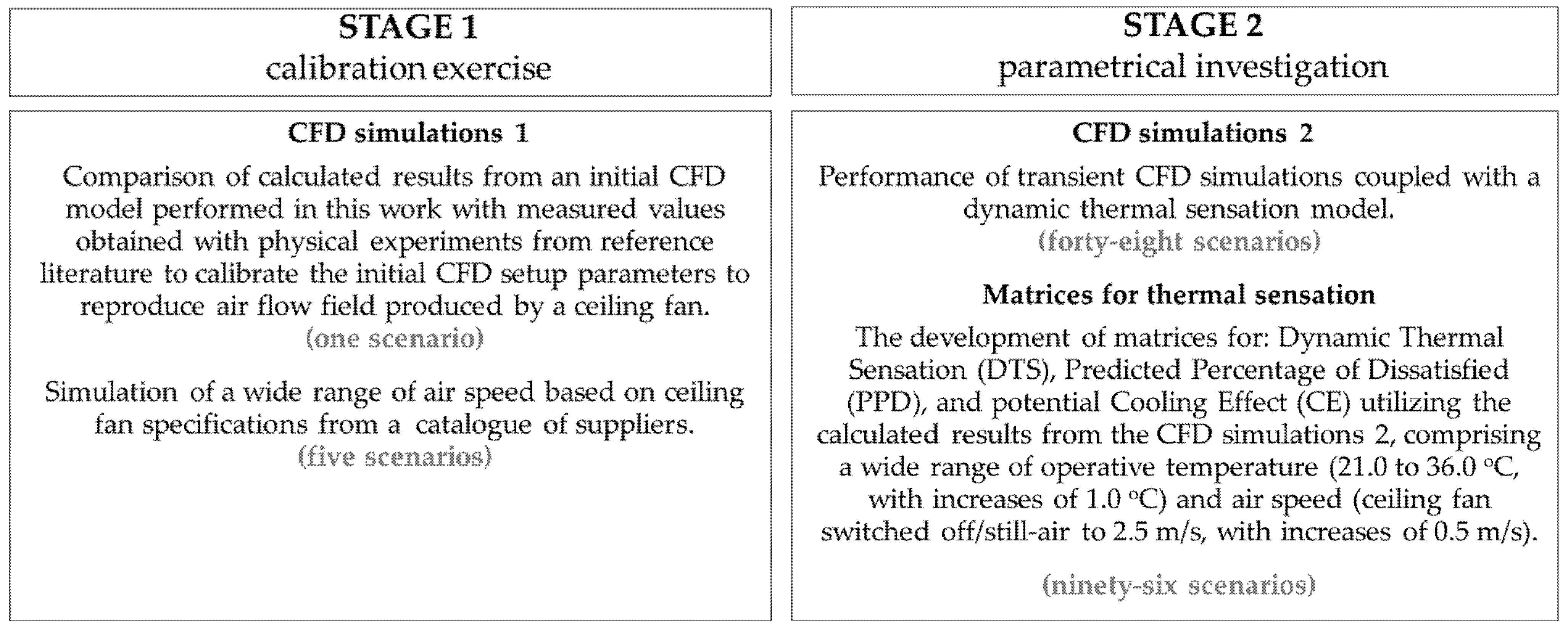
The main objective of this work is to explore the relationship between air speed and operative temperature and the potential to provide (or not) thermal comfort for ranges of values beyond that presented by ASHRAE Standard 55 [6]. Further, this work aims to present three matrices of values related to thermal sensation to quantify the potential comfort (discomfort) sensation for the range of values explored and assist in the design of naturally ventilated low-energy environments.
The research method comprises transient computer fluid dynamics (CFD) simulations coupled with a model to predict thermal sensation and reproduce the airflow field environment of a mechanical ceiling fan. The methodological approach is divided into two stages: a calibration exercise and a parametrical investigation. Initial results from transient CFD simulations are compared with values from field measurements to calibrate the simulation of the airflow field produced by mechanical ceiling fans. Then, based on the results obtained with a large number of transient CFD simulations, coupled with a model for the prediction of thermal sensation performed with a wide range of operative temperatures and air speeds, three matrices of values are obtained. They are: Dynamic Thermal Sensation (DTS) (a computer-based seven-point scale for the prediction of thermal sensation), Predicted Percentage of Dissatisfied (PPD), and potential Cooling Effect (CE), as a resulting effect of forced convective cooling with air movement on the skin.
This paper is structured as follows: Section 1 introduces the research problem; Section 2 describes the research method; Section 3 shows the results for the calibration exercise and presents the matrices of values for DTS, PMV, and CE from the parametrical investigation; Section 4 presents a discussion, highlighting key aspects and practical applications; and Section 5 provides the conclusions.

2. Research Methods

To deliver the results proposed for the main objectives of this work, this research uses transient CFD simulations as a research method that reproduces the flow of a mechanical ceiling fan. The application of the research method is divided into two stages: calibration of initial setup parameters and parametric investigation (Figure 1), with the simulations for Stage 2 coupled with a model for the prediction of thermal sensation.

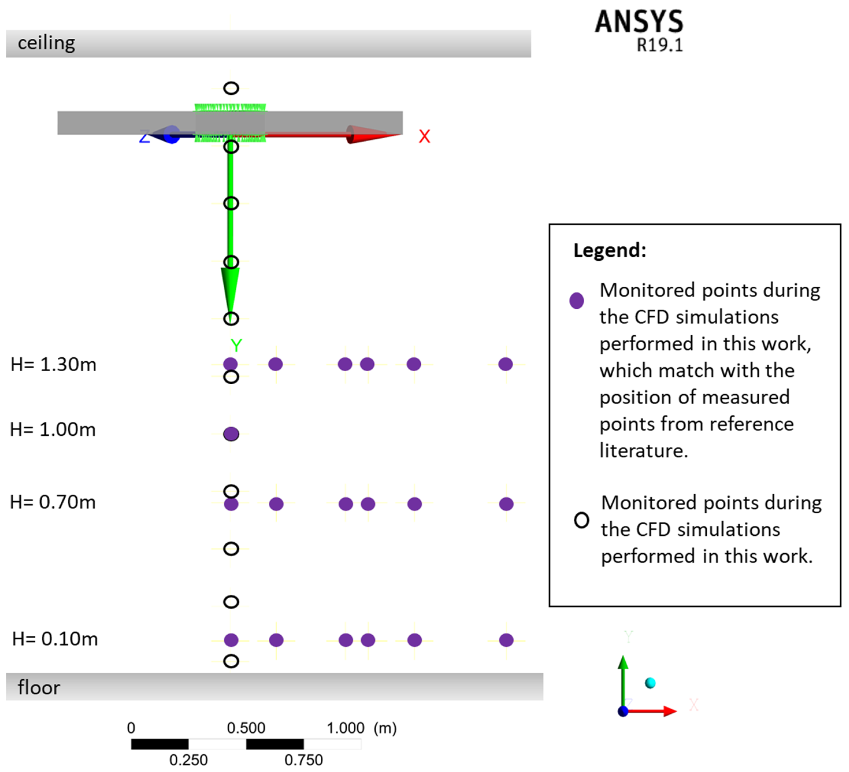
2.1. The Calibration Exercise Setup (Stage 1)

In Stage 1, the calibration exercise comprises the comparison of calculated results from transient CFD models with measured values from physical experiments performed in an environmental chamber, from the reference literature, to calibrate initial CFD setup parameters. With the purpose of calibrating the initial CFD models used in this work, and due to the impossibility of performing physical experiments during the simulation stages due to the COVID-19 pandemic, this work reproduces in CFD the physical experiments performed by Babich et al. [36]. Calculated results for air speed are statistically and quantitatively compared with measured values from this reference literature. Finally, changes in the setup parameters of the modeled fan are carried out to reproduce a wider range of air velocity. These changes are based on ceiling fan specifications for rotations per minute (RPM) from Brazilian suppliers [39].
The virtual model reproduces the physical dimensions of the environmental chamber and the setup parameters of the experiments as described in the reference literature, consisting of an empty room with a ceiling fan placed in its center. Ambient and boundary conditions reproduce informed values for air temperature (31.9 °C) and relative humidity (66%). To reproduce the airflow field produced by a ceiling fan in the CFD simulations momentum sources are assigned for the axial, radial, and theta components of a virtual flat, hollow cylinder modeled with height 0.5 m, radius 0.6 m, and center hole with radius 0.1 m totalizing a sweep of 1.40 m. In the first stage of this work, we reproduce the settings described in the reference literature [36] to, first, calibrate the initial CFD model and, second, change the setup values to calculate other velocity modes for the ceiling fans, based on guidelines for ceiling fans available in the market [39]. The setup parameter that matches the specifications informed in the reference literature corresponds to ‘velocity mode IV’. The other velocity modes are based on the specification informed for typical ceiling fan devices (typically three- or four-blade ceiling fans) from a catalogue for an energy consumption efficiency label. Eventually, the RPM values are obtained with the calculated flow rate and using the First Law of Fans (Equation (1)) [40].
Q2 = Q1 (n/n1)
where Q is airflow rate (m3/s) and n is RPM.
A cross-section of the modeled domain—showing the virtual ceiling fan and the monitored points—is shown in Figure 2, while the setup parameters for the virtual ceiling fans are shown in Table 2.
During the CFD simulations, the calculated air speed was monitored at 19 points for comparison with the measured values. The position of the monitored points matches the location of air speed sensors informed in the reference literature [36] to allow comparison. The points are placed in three rows above the floor (0.10, 0.70, and 1.30 m), with six points placed in line for each row and distributed non-uniformly (center, and 0.20, 0.50, 0.60, 0.80, and 1.20 m). Further, a single point was measured at 1.0 m height on the central axis of the fan. In this work, a further 10 points were added at the vertical axis of the virtual ceiling fan (at 0.25, 0.50, 0.75, 1.25, 1.50, 1.75, 2.00, 2.25, 2.50, and 2.75 m above the floor) to produce a vertical speed profile for all simulated speed modes (Figure 2).

2.2. The Parametric Investigation Setup (Stage 2)

For the parametric investigation performed in Stage 2, the thermal sensation model is coupled to the CFD simulations. The thermal sensation model used is the IESD-Fiala [41,42,43] version 1.4.0, a Linux-based model of human thermophysiology for the prediction of dynamic thermal sensation. The Fiala model, coupled with CFD by Cropper et al. [44], deals with complex human thermoregulation systems interacting with the environment, mathematically reproducing both passive and active thermoregulation systems for the human body. This model utilizes initial values for the metabolic rate based on the activity being performed, clothing insulation levels, air relative humidity, operative temperature, and air speed, to predict values for mean skin temperature, radiant temperature, body metabolic ratio, sweat moisture production, wetted skin area, evaporation due to skin and respiration, blood flow rates, and Dynamic Thermal Sensation (DTS) and PPD thermal comfort indexes. The DTS is a seven-point scale to classify thermal sensation, which is comparable to Fanger’s PMV scale. Conversely, while the latter scale utilizes parameters for individual characteristics (such as clothing level and physical activity level) and for environment characteristics (air temperature, mean radiant temperature, air speed, and air relative humidity) to determine the thermal sensation index (Equation (2)) [6,8], the former scale also considers the rate of change of the mean skin temperature, the body core temperature, and the hypothalamus temperature (Equations (3) and (4)) [12]. These additional parameters used by the IESD-Fiala model drive the passive and active thermoregulation systems and define the overall DTS. A schematic diagram showing the passive and active thermoregulation systems for the human body, as considered in the IESD-Fiala thermal sensation model, is shown in Figure 3. The PPD values can be derived from both the PMV and the DTS seven-point scales utilizing Equation (5) [6,8].
PMV = [0.303 exp(−0.036 M) + 0.028] × {(M − W) − 3.05 × 10⁻³ [5733 − 6.99 (M − W) − pa]
− 0.42 [(M − W) − 58.15] − 1.7 × 10⁻⁵ M (5867 − pa) − 0.0014 M (34 − Tinside)
− 3.96 × 10⁻⁸ ƒcl [(tclm + 273)4 − (Tradmean + 274)4] − ƒcl hc (tclm − Tinside)}
where M is the metabolic rate (in met), W is the effective mechanical power (in W), pa is the water vapor partial pressure (in Pa), Tinside is the air temperature inside (in °C), ƒcl is the clothing surface area factor, tclm is the mean clothing surface temperature (in °C), Tradmean is the mean radiant temperature (in °C), and hc is the convective heat transfer coefficient (in W/m2 K) [6,8].
DTS = 3 tanh{[((0.11 dTskin,m/dt) + 1.91(dTskin,m/dtmax)e − 0.681t)/(1 + G)] + M(Tskin,m − 34.4) + G}
where dTskin,m/dt is the rate of change of the mean skin temperature (in °C) and G is the body core temperature (in °C) [12].
G = 7.94 exp [(−0.902/(Thy − 36.6)) + (7.612/(Tskin,m − 38.4))]
where Thy is the hypothalamus temperature (°C) [12].
PPD = 10–95 exp (−0.03353 PMV4 − 0.2179 PMV2)
The Cooling Effect (CE, in °C) with the convective heat change on the mean skin temperature (Tskin,m) is calculated with the resulting Tskin,m obtained for a given air speed (Vair, in m/s) minus the resulting Tskin,m when the ceiling fan is switched off (still air).
The effectiveness of the used method (transient CFD simulations coupled with the model for thermal sensation) to predict thermal sensation of individuals in naturally ventilated indoor environments located in warm-humid regions has been previously investigated by the authors [45]. In this previous work, the calculated DTS results were compared with benchmark values obtained from questionnaires answered by individuals for thermal sensation votes (TSV) from the reference literature [46,47] and with calculated PMV based on experimental data, and for environmental conditions for a non-residential naturally ventilated building located in a Brazilian warm-humid tropical region. The reported results showed that the calculated DTS values agreed more with the TSV values informed by volunteers than with the PMV values calculated using ASHRAE Standard 55 [6].
In this work, a total of 48 transient CFD simulations coupled with the thermal sensation model were performed in Stage 2. A further 48 points were calculated based on a model which utilizes a weighted average running mean equation to interpolate data [48] totaling 96 values, which are shown in the matrices for DTS, PPD, and CE. While some setup parameters were constant throughout all scenarios simulated (relative humidity at 60%, clothing insulation level at 0.40 clo, and metabolic rate at 1.0 met), air speed ranged from 0 to 2.5 m/s, with increases of 0.5 m/s, while operative temperature ranged from 21.0 °C to 36.0 °C, with increases of 1.0 °C.
All CFD models were built and meshed with ANSYS ICEM R16.0 [49] and solved with ANSYS CFX R19.1 [50] in a high-performance computing facility. The grid independence of the solutions was verified for both virtual environments employed in Stage 1 and Stage 2 using the Fine Grid Convergence Index method, proposed by Celik et al. [51] and Hadjukiewicz et al. [52] to verify and estimate the averaged numerical uncertainty due to discretization errors in CFD simulations. A detailed description of the grid analysis and the CFD simulation setup is provided in previous work from the authors [45].

3. Results

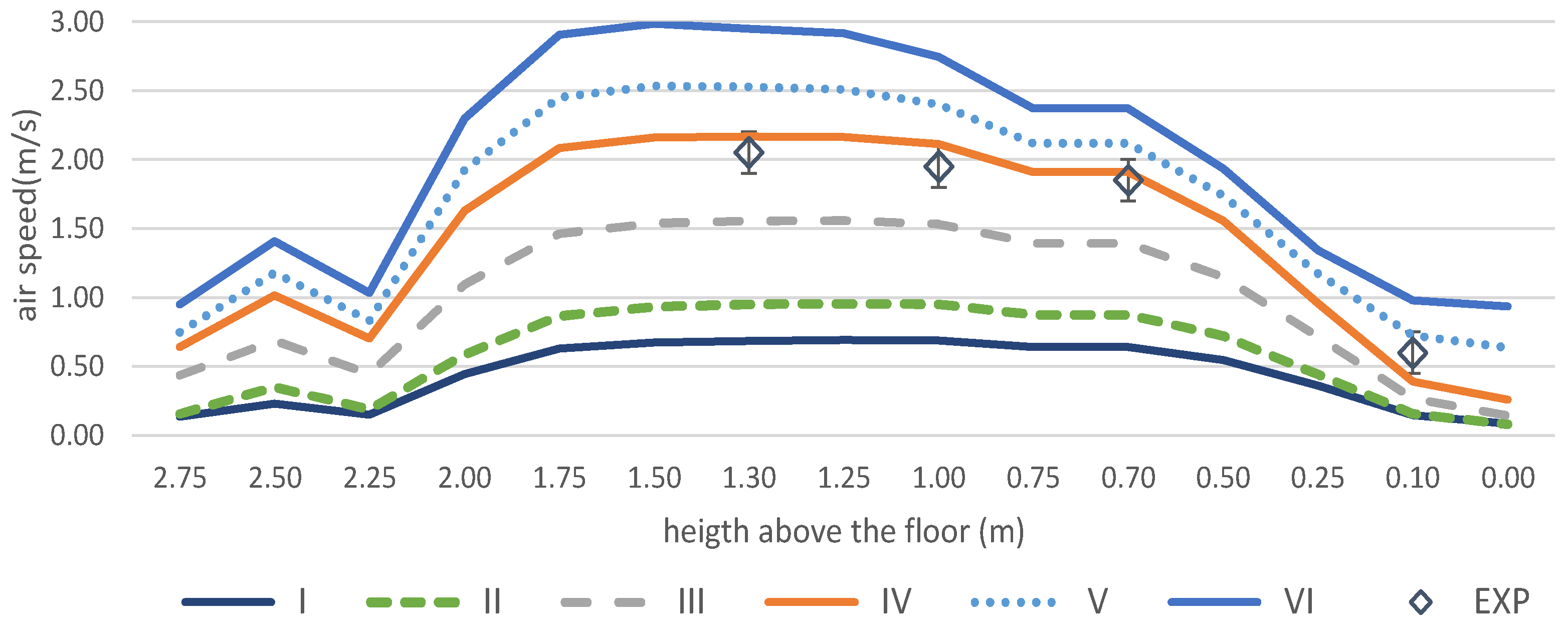
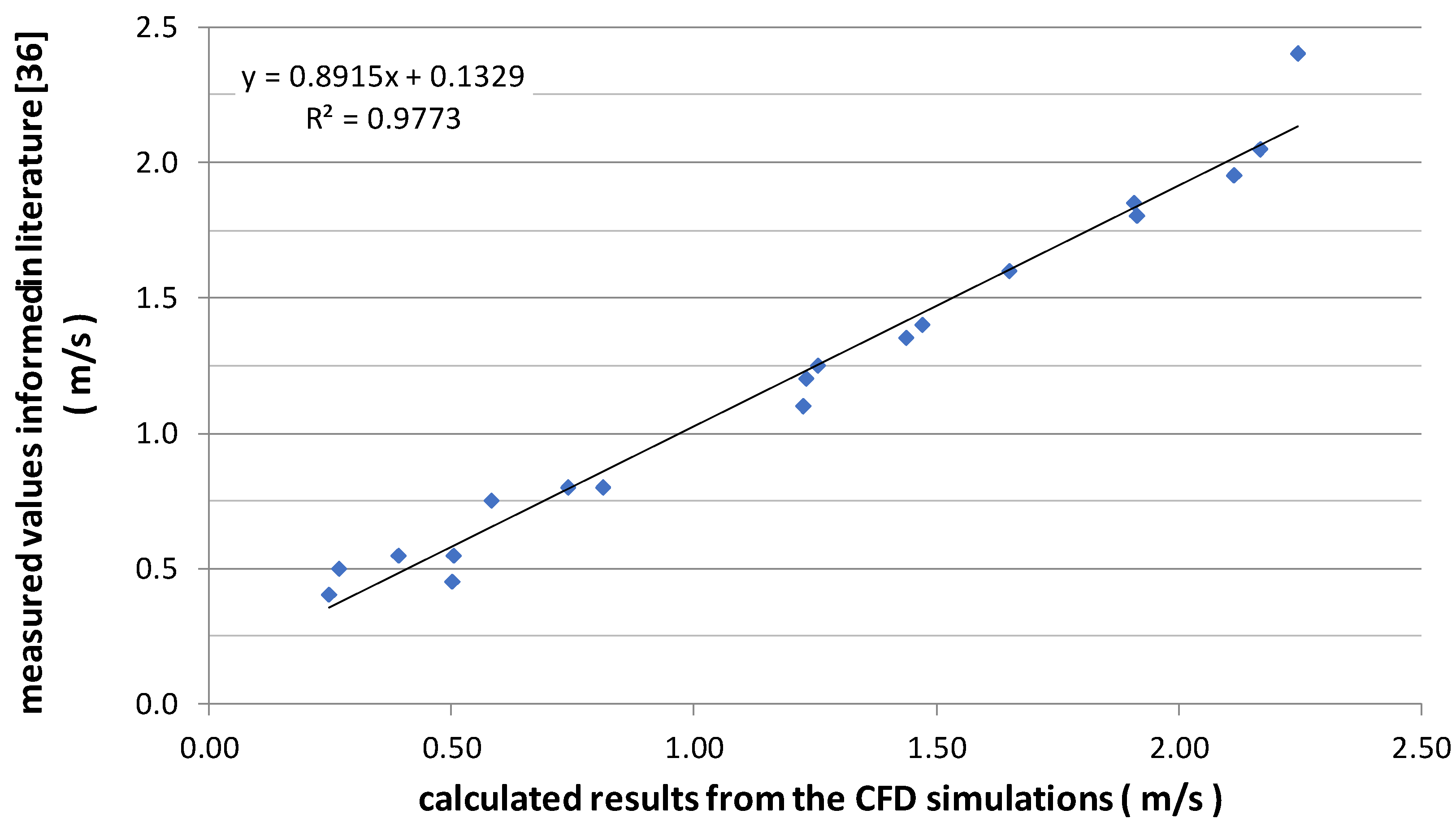
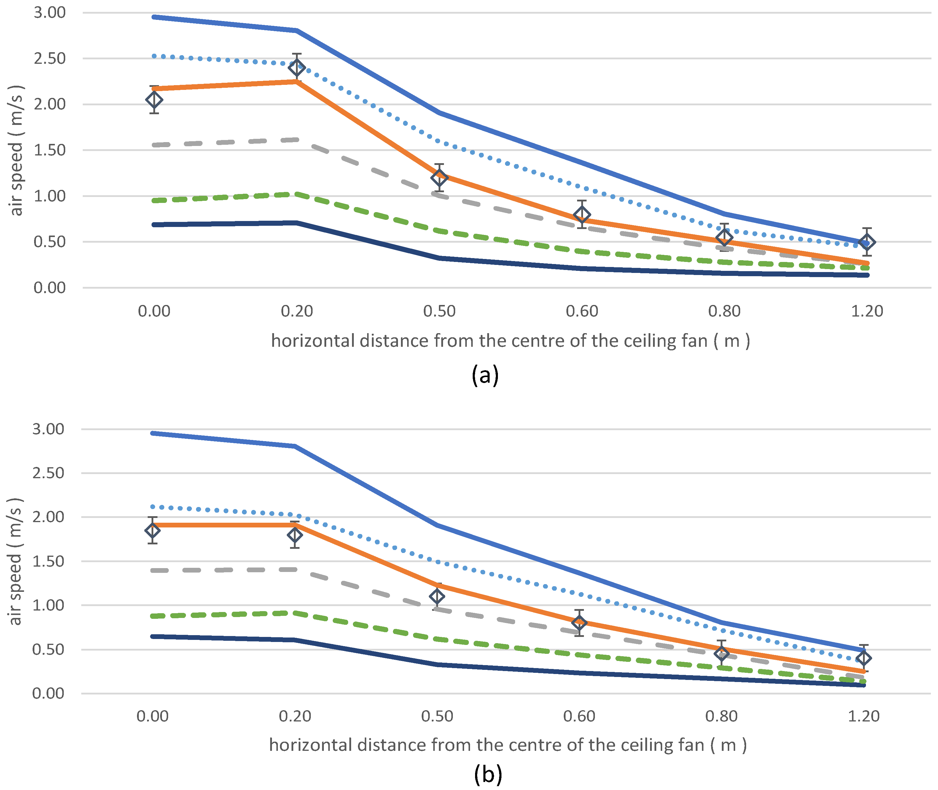
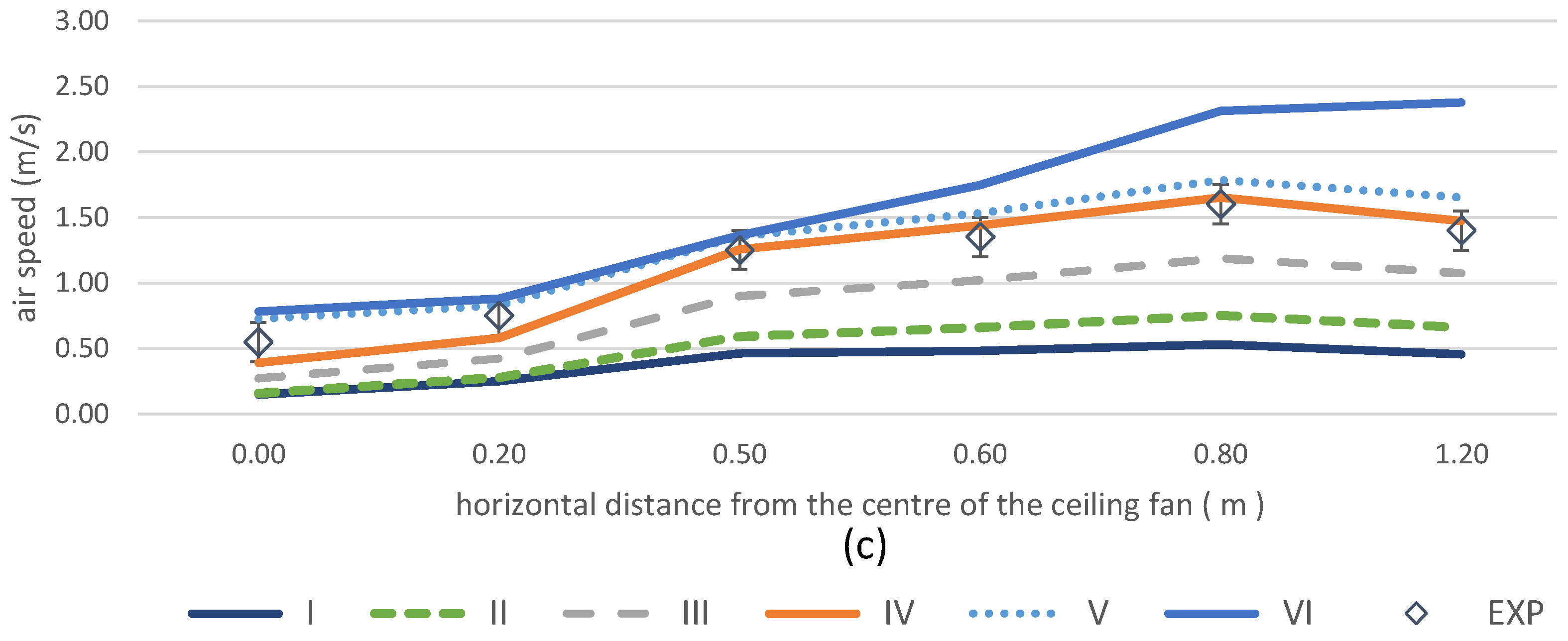
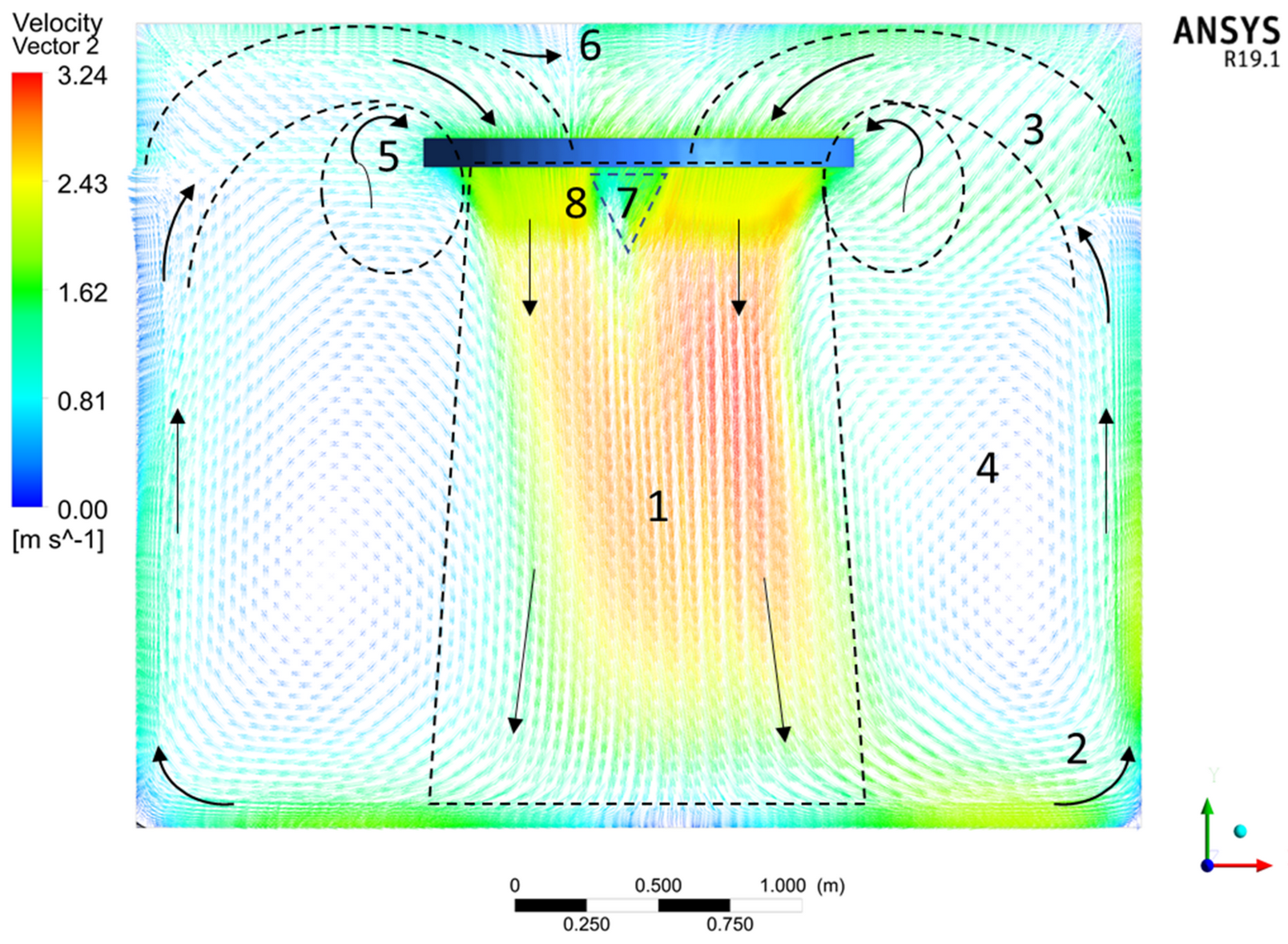
3.1. The Calibration Exercise (Stage 1)

In this section, the results for the calibration exercise are presented and analyzed. First, a quantitative analysis for the comparison of calculated air speed with measured values is shown. Then, a qualitative analysis for the flow field produced by the virtual ceiling fan is provided. The statistical analysis is carried out to identify the statistical strength between the CFD calculated results and the measured values informed in the reference literature [36]. The linear association between the two sources of data is determined by the correlation coefficient (r) and the coefficient of determination (R2) in a scale of significance ranging from +1.00 (perfect correlation) to −1.00 (reverse correlation) [53,54]. The computed correlation coefficient and coefficient of determination indicate that the CFD calculated results are statistically comparable and show a high level of agreement (R2 = 0.98) with the measured values from the reference literature (Figure 4).
Further quantitative analysis shows that 89.5% (17 out of 19 points) of the calculated air speed are within the error bar range of the measured values (accuracy of ±0.03 m/s plus 4%) informed in the reference literature, with the two points being outside the error bar by values less than 0.20 m/s. The calculated air speed for the 19 points is shown in Figure 5 for one vertical profile positioned at the center of the fan and in Figure 6 for three horizontal profiles, positioned parallel to the floor at 0.10 m (Figure 6a), 0.70 m (Figure 6b), and 1.30 m (Figure 6c) above the floor. The calculated results, which are comparable with the measured values informed in the reference literature [36], are those shown in the line for ‘velocity mode IV’, since only this velocity mode used the same setup parameters for the cylindrical components informed in the reference literature. The lines for other velocity modes used other setup parameters for the cylindrical components (for further information, refer to Table 2 in Section 2.1).
The analysis of the vertical profile and the three horizontal profiles shows that the air speed near the center of the fan increases at mid-height (1.3–0.7 m) and reduces near the floor (0.1 m height). The opposite is observed at 1.2 m away from the center (a distance equivalent to twice the length of the blade of the fan), where the air speed near the center of the fan reduces at mid-height and increases near the floor. The airflow rate calculated for velocity modes I to VI ranged from 0.50 to 3.93 m3/s, while the air speed measured at 1.0 m above the floor on the vertical axis of the fan ranged from 0.59 to 2.75 m/s (Table 3).
A qualitative analysis of the flow field produced by the virtual ceiling fan simulated in CFD for the scenario that reproduces the ‘velocity mode VI’ is provided in Figure 7.
The velocity vectors shown in Figure 7 present most of the main features expected from a flow field produced by ceiling fans, which are described in the reference literature [32]. The only exception is the flow in the adjacent entrainment zone near the edge of the fan (5), which is underestimated. Conversely, this underestimation also agrees with the results reported in the reference literature [36]. Further, the flow field is not symmetrical since it represents a cross-section of a two-dimensional snapshot of the dynamic flow field produced in the CFD simulation.
The results of the calibration exercise performed in Stage 1 and presented in this section demonstrate that the selected method to reproduce the flow field produced by a ceiling fan in CFD simulations can deliver calculated results for air speed that are both statistically and quantitatively comparable to measured values from the reference literature. In addition, the simulated flow field develops all the expected features of an actual ceiling fan, which are presented and described in several literature sources. The combined results indicate that the setup used for the CFD modeling is adequate for the analysis proposed in Stage 2, which utilizes transient CFD simulations coupled with a thermal sensation model to analyze the effect of air speed and operative temperature on thermal sensation.

3.2. The Matrices for Thermal Comfort Obtained with Parametric Investigation (Stage 2)

In this section, the ‘matrices for thermal comfort’ named in this work are presented and analyzed. Conversely, before the matrices are presented, Figure 8 shows a two-dimensional snapshot of the dynamic flow field produced by the virtual ceiling fan with the seated manikin simulated in transient CFD coupled with the thermal sensation model. The scenario presented reproduces ‘velocity mode III’ with the operative temperature set at 26.0 °C.
The velocity vectors in Figure 8 show that the introduction of the virtual human manikin in Stage 2 changes some features of the flow field initially simulated for an empty chamber. These changes occur at the descending jet core below the fan and at the spreading zone near the floor, where the manikin is located. Further, the modeling of detailed opening systems for ventilation and actual internal environments, with furniture and partitions (which are not covered in this work), may also change the flow field [24,28]. This change may impact and reduce the efficiency of a proposed ventilation strategy to deliver thermal comfort.
The matrices for thermal comfort are derived from parametric investigation utilizing values from transient CFD simulations coupled with a thermal sensation model. In this parametric investigation, air speed ranged from 0 m/s (still air) to 2.5 m/s with increases of 0.5 m/s, while operative temperature ranged from 21.0 to 36.0 °C with increases of 1.0 °C. The matrices are presented for Dynamic Thermal Sensation (DTS) (Figure 9), Predicted Percentage of Dissatisfied (PPD) (Figure 10), and Cooling Effect (CE) of the air speed on the mean skin temperature (Skm) (Figure 11), with this last matrix based on the comparison of Skm obtained with still air (with the virtual ceiling fan switched off in the CFD simulations).
The matrix for DTS (Figure 9) indicates that neutral thermal sensation (zero) can be potentially obtained with two sets of operative temperature and air speed: 24.0 °C and still air, and 27.0 °C and air at 0.5 m/s. Thermal comfort, ranging from −0.5 to +0.5, can be potentially obtained for a range of 21.0–31.0 °C combined with air speeds up to 2.5 m/s. Environments with operative temperatures above 29.0 °C are highly dependent on increased air speed to provide thermal comfort. Conversely, for operative temperatures above 32.0 °C, increased air speed shows limited or no capacity to mitigate hot/warm thermal sensation. For operative temperatures below 26.0 °C, increased air speed can potentially cause slightly cool/cool thermal sensation. Although this work does not evaluate the effect of adaptive behavior, the presented matrix for DTS shows a clear range for which air speed can potentially deliver thermal comfort; at 31.0 °C, thermal comfort is potentially achievable with air speed of 2.5 m/s, while values from standards indicate that thermal comfort could be achieved with air speeds up to 1.6 m/s.
The matrix for PPD (Figure 10) follows the same pattern observed for the matrix for DTS for the relationship between operative temperature and air speed, with 11 arrangements delivering DTS of 5%, with a range of 24.0–29.0 °C for operative temperature and 0–2.5 m/s for air speed. The matrix for the CE (Figure 11) of air speed on Skm shows that, although the mechanical properties of the air movement produced by the ceiling fan on the skin surface is the same for a given air speed, the resulting cooling effect due to convective heat change may vary considerably according to the operative temperature of the environment. For example, for a given air speed of 2.5 m/s, the values for the CE on Skm range from 0 up to 1.53 °C for a respective operative temperature range of 36.0–21.0 °C. For air speed at 0.5 m/s, the CE on the Skm ranges from 0 up to 0.9 °C for the same range of operative temperatures.
For an operative temperature of 36.0 °C, the cooling effect of air movement on Skm is minimum. Based on the matrices for DTS and PPD, thermal sensation is hot and dissatisfaction is very high (97–98%) for this extremely high temperature, regardless of air speed. For an operative temperature of 31.0 °C, the cooling effect of air movement on Skm ranges from 0.17–0.32 °C, with an air speed range of 0.5–2.5 m/s. Conversely, the effectiveness of the convective heat transfer is considerable. Based on the matrices for DTS and PPD, thermal sensation changes from warm to neutral, whilst dissatisfaction drops from 46 to 10%. For an operative temperature of 21.0 °C, the cooling effect of air movement on Skm ranges from 0.90–1.53 °C, with a range of air speeds of 0.5–2.5 m/s. On the contrary, the thermal sensation changes from neutral to cool, whilst dissatisfaction increases from 8 to 39%.

4. Discussion

Comparison of CFD calculated DTS with PMV values from international standards.
For comparison, PMV was also calculated on the basis of ASHRAE Standard 55 using the Thermal Comfort Tool made available online by the Center for the Built Environment at the University of California [55,56]. The same environmental and individual parameters employed in Stage 2 were used to calculate the PMV values (operative temperature range 21.0–36.0 °C, air speed range OFF–2.5 m/s, relative humidity 60%, metabolic rate 1.0 met, and clothing level 0.4 clo). The PPD values are derived from both the values for the PMV and the DTS seven-point scales. The results for both PPD-PMV and PPD-DTS scales (range 0–100%) are provided for the operative temperature range of 21–36 °C in Figure 12.
In Figure 12, it can be seen that the PPD-PMV values create an inverted Gaussian distribution comparable to the curves for the relationship between the PPD and the PMV values, and for which the overall data are symmetric by the mean, with values near the mean representing the lowest dissatisfaction and values near the edges showing the highest dissatisfaction. Conversely, the PPD-DTS does not follow the typical inverted Gaussian distribution.
The PPD-DTS scale shows a low percentage of dissatisfied individuals when the operating temperature is below 28 °C compared to the PPD-PMV scale. Results between PPD-PMV and PPD-DTS are closer for operative temperatures of 28.0–30 °C regardless of air speed, showing an average dissatisfaction value of 12%. Above 30 °C, the curves for the PPD-DTS scale are similar to the curves for the PPD-PMV scale, with the former values exceeding the latter values by approximately 9%. The distribution curves for the PPD-PMV and PPD-DTS values shown in Figure 12 agree with reported findings [57]. They show that the PPD values derived from observed percentages of unacceptability (OPU) obtained from volunteers are also lower than the PMV values for negative thermal sensation (cold, cool, slightly cool), reflected by low percentages of dissatisfied, while exceeding the PMV values for positive thermal sensation (slightly warm, warm, hot).

5. Conclusions

The main objective of this work was to explore the relationship between air speed and operative temperature and the potential to provide (or not) thermal comfort for ranges of respective values beyond the ones presented by ASHRAE Standard 55.
The research method used transient computer fluid dynamics (CFD) simulations coupled with a model to predict thermal sensation and to reproduce the airflow field environment of a mechanical ceiling fan. The CFD setup was first calibrated with a comparison of calculated results with values from the reference literature, the calculated air speed was statistically and quantitatively comparable to the measured values, and the simulated flow field reproduced the expected features of an actual ceiling fan.
Matrices for thermal comfort were produced with parametric investigation utilizing values from coupled CFD simulations for a range of air speeds (ceiling fan up to 2.5 m/s, with increases of 0.5 m/s) and operative temperatures (21.0 to 36.0 °C, with increases of 1.0 °C), and presented for Dynamic Thermal Sensation (DTS), Predicted Percentage of Dissatisfied (PPD), and cooling effect of the air speed on the mean skin temperature.
Although this work does not evaluate the effect of adaptive behavior, the presented matrices show a clear range for which air speed can potentially deliver thermal comfort. The matrix for DTS shows that a neutral thermal sensation ranging from −0.5 to +0.5 is potentially obtainable for an operative temperature range of 21.0–31.0 °C combined with air speeds up to 2.5 m/s, with environments with operative temperatures above 29.0 °C being highly dependent on increased air speed to deliver thermal comfort.
Additionally, while the increase in air speed shows limited or no capacity to mitigate the hot/warm thermal sensation for an operation temperature above 32.0 °C, it can cause a slightly cool/cool thermal sensation for temperatures below 26.0 °C.
The discussion demonstrated that, while the calculated values underestimate/overestimate the percentages of dissatisfied for operative temperatures below 28 °C and above 31 °C, when compared with the values calculated by international standards, this trend is in accordance with findings reported in the literature for percentages of dissatisfied calculated with observed percentages of unacceptability.
The simulation model and the results provided can be of great help in designing comfortable interior environments for a room’s occupants, as well as in the correct design of either natural ventilation operating concurrently with mechanical ventilation or typical air conditioning systems.

Author Contributions

Conceptualization, L.C.d.F.; funding, L.C.d.F. and M.d.A.R.; methodology, L.C.d.F.; software and validation, L.C.d.F. and C.P.-A.; writing—draft and editing, L.C.d.F., C.P.-A. and P.V.S.; writing—review, L.C.d.F., P.V.S., C.P.-A., M.d.A.R. and L.F.d.S.P.; supervision, M.d.A.R.; project administration, L.C.d.F. All authors have read and agreed to the published version of the manuscript.

Funding

This research is financially supported by the São Paulo Research Foundation—FAPESP (Fundação de Amparo à Pesquisa do Estado de São Paulo) with grant number: 2020/06691-9. The authors express their gratitude for the support received.

Acknowledgments

This work is part of the research, ‘Natural Ventilation and Thermal Comfort for Brazilian Residences’, carried out at the School of Architecture and Urbanism at São Paulo University (FAU USP), Brazil. The researchers would like to express their gratitude to the Institute of Energy and Sustainable Development (IESD) at De Montfort University, UK, which developed the IESD/Fiala model, and to the School of Architecture, Building and Civil Engineering (SABCE) at Loughborough University, UK, for the support with the transient CFD simulations coupled with the IESD/Fiala.

Conflicts of Interest

The authors declare no conflict of interest.

Nomenclatures

ASHRAEAmerican Society of Heating, Refrigerating and Air-Conditioning Engineers
CECooling effect (in °C)
CFDComputer fluid dynamics
CSPSVColor sequence particle streak velocimetry
DTSDynamic thermal sensation
EXPEnvironmental chamber
NVNatural ventilation
OPUPercentages of unacceptability
PMVPredicted mean vote
PPDPredicted percentage of dissatisfied
RACRoom air conditioning
RPMRotations per minute
SkmMean skin temperature (in °C)
TSVThermal sensation votes

References

  1. IEA. The Future of Cooling. Opportunities for Energy-Efficient Air Conditioning. Organisation for Economic Co-operation and Development. International Energy Agency. Available online: http://www.iea.org/publications/freepublication/The_Future_of_Cooling.pdf (accessed on 22 May 2018).
  2. IEA. Cooling. International Energy Agency. Available online: https://www.iea.org/reports/cooling (accessed on 22 May 2018).
  3. CIBSE AM 10. Applications Manual 10: Natural Ventilation; The Chartered Institution of Building Services Engineers: London, UK, 2005. [Google Scholar]
  4. de Faria, L.; Cook, M.; Loveday, D.; Angelopoulos, C.; Shukla, Y.; Rawal, R.; Manu, S.; Mishra, D.; Patel, J.; Saranya, A. Design charts to assist on the sizing of natural ventilation for cooling residential apartments in India. In Proceedings of the BS 2019: 16th IBPSA International Conference & Exhibition, Rome, Italy, 2–4 September 2019; International Building Performance Simulation Association: Wisconsin, WI, USA, 2020. [Google Scholar] [CrossRef]
  5. Cook, M.; Shukla, Y.; Rawal, R.; Loveday, D.; de Faria, L.C.; Angelopoulos, C. Low Energy Cooling and Ventilation for Indian Residences Design Guide; CEPT Research and Development Foundation—CRDF: Ahmedabad, India, 2020; Volume 1, 61p, ISBN 978-1-8380310-0-8. [Google Scholar]
  6. ASHRAE/ANSI Standard-55. Thermal Environmental Conditions for Human Occupancy; American Society of Heating and Air-Conditioning Engineers: Atlanta, GA, USA, 2017. [Google Scholar]
  7. Fanger, P.O. Thermal Comfort; Danish Technical Press: Copenhagen, Denmark, 1970; ISBN 9780070199156. [Google Scholar]
  8. ISO 7730. Ergonomics of the Thermal Environment—Analytical Determination and Interpretation of Thermal Comfort Using Calculation of the PMV and PPD Indices and Local Thermal Comfort Criteria; International Standard Organization: Geneva, Switzerland, 2005. [Google Scholar]
  9. Callahan, M.; Gum, H. Development of a High Efficiency Ceiling Fan. In Proceedings of the Twelfth Symposium on Improving Building Systems in Hot and Humid Climates, San Antonio, TX, USA, 15–17 May 2000; pp. 270–277. [Google Scholar]
  10. Santamouris, M. Ceiling Fans; AIVC—Air Infiltration and Ventilation Centre: Sint-Stevens-Woluwe, Belgium, 2007; pp. 1–12. [Google Scholar]
  11. Santamouris, M. Ventilation for Comfort and Cooling: The State of the Art. In Building Ventilation: The State-of-the-Art; Santamouris, M., Wouters, P., Eds.; Earthscan: London, UK, 2007; pp. 217–246. [Google Scholar] [CrossRef]
  12. Fiala, D.; Psikuta, A.; Jendritzky, G.; Paulke, S.; Nelson, D.; Van Marken Lichtenbelt, V.; Frijns, A. Physiological modeling for technical, clinical and research applications. Front. Biosci. 2010, 1, 939–968. [Google Scholar] [CrossRef] [PubMed] [Green Version]
  13. Scheatzle, D.G.; Wu, H.; Yellott, J. Extending the summer comfort envelope with ceiling fans in hot arid climates. ASHRAE Trans. 1989, 95, 269–280. [Google Scholar]
  14. Mallic, F.H. Thermal comfort and building design in the tropical climates. Energy Build. 1996, 23, 161–167. [Google Scholar] [CrossRef]
  15. de Dear, R.; Brager, G.S.; Cooper, D. Developing an adaptive model of thermal comfort and preference. In ASHRAE RP-884 Final Report; American Society of Heating and Air-Conditioning Engineers: Atlanta, GA, USA, 1997; Available online: https://escholarship.org/uc/item/4qq2p9c6 (accessed on 18 September 2020).
  16. de Dear, R.; Kim, J.; Parkinson, T. Residential Adaptive Comfort in a Humid Subtropical Climate—Sydney Australia. Energy Build. 2018, 158, 1296–1305. [Google Scholar] [CrossRef]
  17. de Dear, R.; Brager, G.S. Thermal comfort in naturally ventilated buildings: Revisions to ASHRAE Standard 55. Energy Build. 2002, 34, 549–561. [Google Scholar] [CrossRef] [Green Version]
  18. Chandra, S.; Fairey, P.; Houston, M. Cooling with Ventilation; Solar Energy Research Institute, U.S. Department of Energy: Cocoa, FL, USA, 1986.
  19. Mcintyre, D. Preferred air speed for comfort in warm conditions. ASHRAE Trans. 1978, 84, 264–277. [Google Scholar]
  20. Rohles, F.; Konz, S.; Jones, B. Ceiling fans as extenders of the summer comfort envelope. ASHRAE Trans. 1983, 89, 245–263. [Google Scholar]
  21. Indraganti, M. Behavioural adaptation and the use of environmental controls in summer for thermal comfort in apartments in India. Energy Build. 2010, 42, 1019–1025. [Google Scholar] [CrossRef]
  22. Indraganti, M. Adaptive use of natural ventilation for thermal comfort in Indian apartments. Build. Environ. 2010, 45, 1490–1507. [Google Scholar] [CrossRef]
  23. Indraganti, M.; Ooka, R.; Rijal, H. Significance of air movement for thermal comfort in warm climates: A discussion in Indian context. In Proceedings of the 7th Windsor Conference: The Changing Context of Comfort in an Unpredictable World, Cumberland Lodge, Windsor, UK, 12–15 April 2012. [Google Scholar]
  24. Gao, Y.; Zhang, H.; Arens, E.; Present, E.; Ning, B.; Zhai, Y.; Pantelic, J.; Luo, M.; Zhao, L.; Raftery, P.; et al. Ceiling fan air speeds around desks and office partitions. Build. Environ. 2017, 124, 412–440. [Google Scholar] [CrossRef] [Green Version]
  25. Liu, S.; Lipczynska, A.; Schiavon, S.; Arens, E. Detailed experimental investigation of air speed field induced by ceiling fans. Build. Environ. 2018, 142, 342–360. [Google Scholar] [CrossRef] [Green Version]
  26. Raftery, P.; Douglass-James, D. Ceiling Fan Design Guide; University of California Berkeley, The Centre for the Built Environment: Berkeley, CA, USA, 2020; Available online: https://escholarship.org/uc/item/6s44510d (accessed on 21 June 2021).
  27. Oh, W.; Kato, S. The effect of airspeed and wind direction on human’s thermal conditions and air distribution around the body. Build. Environ. 2018, 141, 103–116. [Google Scholar] [CrossRef]
  28. Raftery, P.; Fizer, J.; Chen, W.; He, Y.; Zhang, H.; Arens, E.; Schiavon, S.; Paliaga, G. Ceiling fans: Predicting indoor air speeds based on full scale laboratory measurements. Build. Environ. 2019, 155, 210–223. [Google Scholar] [CrossRef] [Green Version]
  29. Falahat, A. Optimization of Flow Coefficient in Tubeaxial Fan at a Different Hub to Tip Ratio. Int. Rev. Mech. Eng. 2011, 5, 1095–1101. [Google Scholar]
  30. Adeeb, E.; Maqsood, A.; Mushtaq, A. Effect of Number of Blades on Performance of Ceiling Fans. In MATEC Web of Conferences; EDP Sciences: Les Ulis, France, 2015; Volume 28, Available online: http://www.matec-conferences.org/10.1051/matecconf/20152802002 (accessed on 15 January 2018).
  31. Schmidt, K.; Patterson, D. Performance Results for a High Efficiency Tropical Ceiling Fan and Comparisons with Conventional Fans Demand Side Management via Small Appliance Efficiency. Renew. Energy 2001, 22, 169–176. Available online: www.elsevier.com/locate/renene (accessed on 22 January 2018). [CrossRef]
  32. Jain, A.; Upadhyay, R.R.; Chandra, S.; Saini, M.; Kale, S. Experimental investigation of the flow field of a ceiling fan. In Proceedings of the ASME 2004 Heat Transfer/Fluids Engineering Summer Conference, Charlotte, NC, USA, 11–15 July 2004; American Society of Mechanical Engineers. pp. 93–99. [Google Scholar]
  33. Wang, H.; Zhang, H.; Hu, X.; Luo, M.; Wang, G.; Li, X.; Zhu, Y. Measurement of airflow pattern induced by ceiling fan with quad-view colour sequence particle streak velocimetry. Build. Environ. 2019, 152, 122–134. [Google Scholar] [CrossRef] [Green Version]
  34. Ge, H.W.; Norconk, M.; Lee, S.Y.; Naber, J.; Wooldridge, S.; Yi, J. PIV measurement and numerical simulation of fan-driven flow in a constant volume combustion vessel. Appl. Therm. Eng. 2014, 64, 19–31. [Google Scholar] [CrossRef]
  35. Babich, F.; Cook, M.; Loveday, D.; Cropper, P. Numerical modelling of thermal comfort in non-uniform environments using real-time coupled simulation models. In Proceedings of the Building Simulation and Optimisation 2016: 3rd IBPSA-England Conference, BPSA, Newcastle upon Tyne, UK, 12–14 September 2016; pp. 4–11. [Google Scholar]
  36. Babich, F.; Cook, M.; Loveday, D.; Rawal, R.; Shukla, Y. Transient three-dimensional CFD modelling of ceiling fans. Build. Environ. 2017, 123, 37–49. [Google Scholar] [CrossRef] [Green Version]
  37. Li, J.; Hou, Y.; Liu, J.; Wang, Z.; Li, F. Window purifying ventilator using a cross-flow fan: Simulation and optimization. Build. Simul. 2016, 9, 481–488. [Google Scholar] [CrossRef]
  38. Chen, Q.; Liu, S.; Gao, Y.; Zhang, H.; Arens, E.; Zhao, L.; Liu, J. Experimental and numerical investigations of indoor air movement distribution with an office ceiling fan. Build. Environ. 2018, 130, 14–26. [Google Scholar] [CrossRef] [Green Version]
  39. Procel. Ventiladores de Teto. Selo Procel: Programa Nacional de Conservação de Energia Elétrica. Centro Brasileiro de Informação de Eficiência Energética. Eletrobrás. 06/08/2019. Available online: http://www.procelinfo.com.br/ (accessed on 22 October 2019).
  40. DOE. Improving Fan System Performance: A Sourcebook for Industry; The U.S. Department of Energy Efficiency and Renewable Energy (EERE), the Department of Energy’s (DOE) Industrial Technologies Program and the Air Movement and Control Association (AMCA): Washington, DC, USA, 2003; 92p. Available online: https://www.nrel.gov/docs/fy03osti/29166.pdf (accessed on 3 September 2020).
  41. Fiala, D.; Lomas, K.; Stohrer, M. Dynamic Simulation of Human Heat Transfer and Thermal Comfort. Ph.D. Thesis, De Montfort University, Leicester, UK, June 1998. Available online: http://hdl.handle.net/2086/4129 (accessed on 28 December 2020).
  42. Fiala, D.; Lomas, K.; Stohrer, M. Computer prediction of human thermoregulatory and temperature responses to a wide range of environmental conditions. Int. J. Biometeorol. 2001, 45, 143–159. [Google Scholar] [CrossRef] [PubMed]
  43. Fiala, D.; Lomas, K.; Stohrer, M. First Principles Modeling of Thermal Sensation Responses in Steady-State and Transient Conditions. ASHRAE Trans. 2003, 109, 179–186. [Google Scholar]
  44. Cropper, P.; Yang, T.; Cook, M.; Fiala, D.; Yousaf, R. Coupling a model of human thermoregulation with computational fluid dynamics for predicting human-environment interaction. J. Build. Perform. Simul. 2010, 3, 233–243. [Google Scholar] [CrossRef] [Green Version]
  45. de Faria, L.C.; Romero, M.; Pirró, L. Evaluation of a Coupled Model to Predict the Impact of Adaptive Behaviour in the Thermal Sensation of Occupants of Naturally Ventilated Buildings in Warm-Humid Regions. Special Issue ‘Indoor Environment in Sustainable Buildings’. Sustainability 2020, 13, 255. [Google Scholar] [CrossRef]
  46. Lamberts, R.; Andreasi, W.A. Thermal Comfort in Buildings Located in Regions of Hot and Humid Climate of Brazil. Laboratory of Energy Efficiency in Buildings, LABEEE. UFSC. 2009. Available online: https://www.researchgate.net/publication/242253258_Thermal_comfort_in_buildings_located_in_regions_of_hot_and_humid_climate_of_Brazil/references (accessed on 10 May 2020).
  47. Andreasi, W.A.; Lamberts, R.; Cândido, C. Thermal acceptability assessment in buildings located in hot and humid regions in Brazil. Build. Environ. 2010, 45, 1225–1232. [Google Scholar] [CrossRef]
  48. de Dear, R. Recent Enhancements to the Adaptive Comfort Standard in ASHRAE 55-2010. In Proceedings of the 45th Annual Conference of the Architectural Science Association, ANZAScA 2011, Sydney, Australia, 14–16 November 2011. [Google Scholar]
  49. ANSYS. ANSYS ICEM CFD R16.0. ANSYS, Inc., 2016. Available online: https://www.ansys.com/training-center/course-catalog/fluids/introduction-to-ansys-icem-cfd (accessed on 19 January 2022).
  50. ANSYS. ANSYS CFX R19.1. ANSYS, Inc., 2018. Available online: https://www.ansys.com/products/fluids/ansys-cfx/ (accessed on 19 January 2022).
  51. Celik, L.; Ghia, U.; Roache, P.; Freitas, C.; Coleman, H.; Raad, P. Procedure for estimation and reporting of uncertainty due to discretization in CFD applications. J. Fluids Eng. Trans. 2008, 130, 0780011–0780014. [Google Scholar] [CrossRef] [Green Version]
  52. Hajdukiewicz, M.; Geron, M.; Keane, M. Formal calibration methodology for CFD models of naturally ventilated indoor environments. Build. Environ. 2013, 59, 290–302. [Google Scholar] [CrossRef] [Green Version]
  53. Naghshpour, S. Statistics for Economics; Business Expert Press: New York, NY, USA, 2012; p. 475. [Google Scholar]
  54. Croft, A.; Davison, R. Foundation Maths, 5th ed.; Pearson: Harlow, UK, 2010. [Google Scholar]
  55. Tartarini, F.; Schiavon, S.; Cheung, T.; Hoyt, T. CBE Thermal Comfort Tool: Online tool for thermal comfort calculations and visualizations. SoftwareX 2020, 12, 100563. [Google Scholar] [CrossRef]
  56. CBE. Thermal Comfort Tool. Available online: https://comfort.cbe.berkeley.edu/ (accessed on 21 July 2021).
  57. Cheung, T.; Schiavon, S.; Parkinson, T.; Li, P.; Brager, G. Analysis of the accuracy on PMV—PPD model using the ASHRAE Global Thermal Comfort Database II. Build. Environ. 2019, 153, 205–217. [Google Scholar] [CrossRef] [Green Version]
Figure 1. Schematic representation of the methodological approach and the stages performed for this work.
Buildings 12 00101 g001
Figure 2. Schematic cross-section of the three-dimensional modeled domain showing the virtual ceiling fan and the points monitored during the CFD simulations performed in Stage 1.
Buildings 12 00101 g002
Figure 3. Schematic diagram showing the passive and active thermoregulation systems for the human body, as considered in the IESD-Fiala model reprinted from Ref. [45].
Buildings 12 00101 g003
Figure 4. Statistical strength between the calculated results from the CFD simulations with the measured values informed in the reference literature [36] for air speed (in m/s).
Buildings 12 00101 g004
Figure 5. Vertical profile of the air speed. The CFD calculated results are shown for a range of six velocity modes, with the results for ‘velocity mode IV’ being comparable to the values measured in an environmental chamber (EXP) provided in the reference literature [36].
Buildings 12 00101 g005
Figure 6. Horizontal air speed profiles placed at 1.30 m (a), 0.70 m (b), and 0.10 m (c) above the floor. The CFD calculated results are shown for a range of six velocity modes, with the results for ‘velocity mode IV’ being comparable to the values measured in an environmental chamber (EXP) provided in the reference literature [36].
Buildings 12 00101 g006aBuildings 12 00101 g006b
Figure 7. Two-dimensional snapshot of the dynamic flow field produced by the virtual ceiling fan simulated in CFD for ‘velocity mode VI’. The main features of the flow are: (1) the descending jet core below the fan, (2) the spreading zone near the floor, (3) the ascending flow near the walls, (4) the recirculation zones, (5) the adjacent entrainment, (6) the suction zone in the top, (7) the zone blocked by the motor, and (8) the local air recirculation near the blades and the motor, as described in the reference literature [32].
Buildings 12 00101 g007
Figure 8. Two-dimensional snapshot of the dynamic flow field produced by the virtual ceiling fan simulated in transient CFD coupled with the thermal comfort model. The scenario reproduces ‘velocity mode III’ with the operative temperature set at 26.0 °C.
Buildings 12 00101 g008
Figure 9. Matrix for Dynamic Thermal Sensation (DTS) from −3.0 to +3.0 for a range of operative temperatures (21.0 to 36.0 °C, with increases of 1.0 °C) and air speeds (ceiling fan switched off/still air to 2.5 m/s, with increases of 0.5 m/s).
Buildings 12 00101 g009
Figure 10. Matrix for Predicted Percentage of Dissatisfied (PPD) from 0% to 100% for a range of operative temperatures (21.0 to 36.0 °C, with increases of 1.0 °C) and air speeds (ceiling fan switched off/still air to 2.5 m/s, with increases of 0.5 m/s).
Buildings 12 00101 g010
Figure 11. Matrix for the Cooling Effect (CE) of air speed on mean skin temperature (Skm) for zero to >1.50 °C for a range of operative temperatures (21.0 to 36.0 °C, with increases of 1.0 °C) and air speeds (ceiling fan switched off/still air to 2.5 m/s, with increases of 0.5 m/s).
Buildings 12 00101 g011
Figure 12. Relationship between the PPD values calculated from the predicted mean vote (PPD-PMV) and from the seven-point dynamic thermal sensation scales (PPD-DTS) (vertical axis) versus the range of operative temperatures (21.0–36.0 °C), shown for the air speed range (OFF–2.5 m/s) covered in this work.
Buildings 12 00101 g012
Table 1. The corresponding increase in the acceptable operative temperature with the increase in air speed, keeping the thermal sensation within the comfort zone (PMV of −0.5, +0.5). Upper limits indicated for an initial operative temperature of 27.00 °C, considering clo and 1.1 met. Values estimated using ASHRAE Standard 55 [6].
Air Speed (m/s)Corresponding Rise in the Operative Temperature (°C)Upper Limit for the Operative Temperature (°C)
0.1-27.00
0.62.8029.80
0.93.4030.40
1.23.7530.75
1.54.0031.00
Table 2. The setup parameters used for the virtual ceiling fan in the transient CFD simulations performed in Stage 1.
VelocityMomentum Sources for the Cylindrical Components
(kg/m2 s2)
ModesAxialRadialTheta
Velocity VI55.000.08.00
Velocity V38.500.05.60
Velocity IV27.500.04.00
Velocity III13.750.02.00
Velocity II5.500.00.80
Velocity I2.750.00.40
Table 3. Calculated results from the virtual ceiling fan for rotations per minute (RPM), airflow rate across the fan, and air speed at 1.0 m above the floor, shown for each velocity mode used for the transient CFD simulations performed in Stage 1.
Velocity ModeRPMMomentum Sources for the Cylindrical Components Air Speed
at 1.0 m
Flow Rate
Axial
(kg/m2 s2)
Radial
(kg/m2 s2)
Theta
(kg/m2 s2)
Above Floor
(m/s)
(m3/s)
Velocity VI33055.000.08.002.753.93
Velocity V26038.500.05.602.403.09
Velocity IV21027.500.04.002.112.50
Velocity III13013.750.02.001.531.55
Velocity II955.500.00.800.951.13
Velocity I422.750.00.400.590.50
Publisher’s Note: MDPI stays neutral with regard to jurisdictional claims in published maps and institutional affiliations.

