
Probabilistic Moment Bearing Capacity Model and Fragility of Beam-Column Joints with Cast Steel Stiffeners

1
School of Civil and Transportation Engineering, Beijing University of Civil Engineering and Architecture, Beijing 100044, China
2
Department of Civil and Environmental Engineering, University of Illinois at Urbana-Champaign, Urbana, IL 61801, USA
*
Author to whom correspondence should be addressed.
Buildings 2022, 12(5), 577; https://doi.org/10.3390/buildings12050577
Submission received: 31 March 2022
/
Revised: 22 April 2022
/
Accepted: 26 April 2022
/
Published: 29 April 2022
(This article belongs to the Section Building Structures)
Abstract
:Beam-column joint with cast steel stiffeners (CSS) is a new type of joint with a large degree of design freedom. The joint stress distribution can be improved by designing a reasonable cross-sectional shape of the CSS with high rigidity, high integrity, and good seismic performance. Due to the construction specificity, the exact theoretical formula for the moment bearing capacity of the CSS joint is hard to deduce. Some researchers have proposed empirical or simplified theoretical formulas for the prediction of moment bearing capacity. However, the formulas are biased and cannot capture uncertainties in the data measurement and modeling process. In addition, current formulas cannot be updated efficiently over time, and no work has been conducted regarding the reliability of the CSS joints subject to different loading conditions. In this paper, a new approach to address the above issues is proposed. A probabilistic model for the joint capacity is established to capture the uncertainties and correct the bias. A Bayesian method is proposed for model training, which allows the model to be updated efficiently whenever new experiment or simulation data are available. A fragility analysis is conducted using the proposed capacity model to quantify the failure probability of joints under different loading conditions. The advantages of the proposed approach are validated by analyzing joints in a database obtained from experiments and numerical simulations. Results show that the proposed capacity model provides unbiased and more accurate estimates of the bending moment than the currently available ones. New factors such as column thickness and concrete filling are found to significantly impact the moment capacity. The bending fragility of CSS joints can be lowered at different degrees by increasing concrete strength, steel strength, column thickness, etc. Guidance on CSS joint design and retrofitting based on the capacity model and fragility analysis is also presented at the end of this paper.
1. Introduction
In steel structures, beam-column joints are required to adapt to the shape of column sections. Most joints are connected with H-shaped columns or tube columns [1,2,3,4]. In recent years, tube columns with square or circular sections have been widely used in practice [5,6,7,8,9]. The main types of joints connecting steel tube columns and H-shaped steel beams are fully welded joints, inner diaphragm joints, outer ring plate joints, diaphragm-through joints, vertical stiffener joints, T-shaped stiffeners, and so on. These joints have greatly enriched the variety of steel tube column joints. However, there are also some problems such as unclear force transmission path, complicated construction, difficult processing, excessively large size, close or intersecting welding seams, large heat-affected zones of welding in joint regions of a steel tube column, tube cutting requirements, etc.
In order to solve the above problems, an H-shaped beam to square tube column joint with cast steel stiffeners (CSS) (shown in Figure 1a) was proposed [8]. The CSS consists of three parts: (i) a ring plate connected to a steel tube, (ii) flanges connected to flanges of the H-shaped steel beam, and (iii) stiffening ribs between the ring plate and the flanges. The reinforcing ribs are rounded to reduce the stress concentrations induced by the stiffeners. The ring plate is provided with a prefabricated welding groove that is connected to a square steel column by a non-penetration butt weld applied along the pre-formed welding groove. Beam flanges are connected to CSS flanges by butt welds, and beam girder webs are connected to column webs by two side fillet welds. The flat surface of the upper CSS has the same height as the upper surface of the beam flange. The presence of CSS has no effect on other aspects of construction, e.g., metal decking and floor slabs. The stiffener can be considered a section of a beam flange during the process of construction. The CSS joint in a real structure is shown in Figure 1b. This beam-column joint with CSS has a convenient production method and a simple installation process.
Due to the construction difference between the CSS joint and normal joints, numerous experimental and analytical studies have been conducted to obtain a relatively clear understanding of the force transfer mechanism and moment bearing capacity of beam-column joints with CSS. Kenzo et al. [8,10] conducted a uniaxial tensile bearing capacity test to investigate the influence of the joint shape on the mechanical properties of the joint and to determine the optimal joint shape. On this basis, a formula for the bearing capacity of the CSS joint was proposed based on the yield line theory through a full-scale low-cycle reciprocating load pseudo-static test on a CSS joint. After that, Eijiro et al. [11] revised the formula and verified the bearing capacity formula through a uniaxial tensile bearing capacity test. Moreover, Yuzo et al. [12] proved that high-strength cast steel material and a square steel tube filled with concrete could reduce the local deformation of the steel tube column and improve the joint bearing capacity through the uniaxial tensile bearing capacity test. Masato et al. [13] conducted a low-cycle reciprocating loading test on a CSS joint and proved that the effect of axial force on the mechanical properties of the joint is mainly manifested after the joint yields, and the axial force has little effect on the mechanical performance of the joint before the joint yields. Based on these studies, Han et al. [5,14,15,16,17] conducted a large number of numerical analyses and experimental research into the mechanical properties of a CSS joint under monotonic and reciprocating loads. The results showed that the load-bearing capacity of the CSS joint is mainly borne by the cast steel connector ring plate, and the load borne by the square steel tube column front plate is negligible. Combined with yield line theory and the deformation coordination principle, a simplified theoretical model was deduced.
The above research results aimed to conclude the bearing capacity with empirical or simplified theoretical models. However, force transfer mechanism analyses in the literature show that the greater overall stiffness and strength of the CSS limit the deformation of the column front shell. The stress redistribution and the deformation pattern of CSS joints are very different compared with welded joints without stiffeners. Due to this unique stress distribution and deformation pattern, one or more formulas are hard to calculate the exciting moment bearing capacity of the CSS joint.
The limitations of the formulas for moment bearing capacity in the literature can be summarized as the following: First, all the formulas mentioned above are empirical or simplified theoretical models without a comprehensive exploratory data analysis. Therefore, it is likely that some important variables that impact the joint performance are missing. For example, none of the past models consider the diameter and thickness of columns in the formula, which implies that the capacity estimates may be inaccurate when the column geometry changes greatly. Second, the estimates of moment capacity from these models are deterministic and always biased. It is, therefore, difficult to obtain accurate estimates or quantify the uncertainties using these formulas. Third, these formulas cannot be updated efficiently over time when new data become available, again due to the deterministic model form and parameters. Last, no work has been conducted regarding the reliability of the joints with CSS under different loading conditions.
To address the above-mentioned issues, a probabilistic capacity model is proposed to capture the uncertainties in this paper, and a Bayesian approach [18,19,20,21,22,23,24,25,26,27,28,29] is developed for model calibration such that the model provides unbiased estimates and can be updated consistently over time. An importance analysis technique is presented that quantifies the importance of different variables in the model. A fragility analysis is then conducted using the capacity model to obtain the failure probability of the joints under different loading conditions. This paper also demonstrates the methods to (1) obtain the moment capacity estimate with an arbitrary exceeding probability p%, (2) grasp how the fragilities vary by different characteristics of the joints, and (3) provide different designing or retrofitting plans with the same reliability.
The rest of this paper is organized as follows: Section 2 discusses the data used for capacity modeling and fragility analysis in this paper. Section 3 reviews the theoretical capacity formula in the literature and discusses the limitations. Section 4 presents the proposed approach, including the methods to develop, train, and analyze a probabilistic capacity model, and estimate the fragility based on such a model. Section 5 implements the proposed approach into practice using the data prepared in Section 2 and analyzes the results. The last section concludes the contributions of this paper.
2. Data Preparation
To study the performance of the bearing moment capacity models proposed in this paper or previous research, experimental and numerical simulation data of the beam-column joint with CSS from reference [5] were collected to form a database. In the database, Joints 1–11 are test specimens, and Joints 12–57 are numerical simulation models. All the experiment specimens were constructed by the same manufactory in the same batch, and the numerical simulation method was validated to be able to simulate the specimens accurately [5]. Joints 1–8 and Joints 12–37 connect H-shaped steel beams and steel tube columns without concrete filled inside, while Joints 9–11 and Joints 38–57 connect H-shaped steel beams and steel tube columns filled with concrete inside. Low-strength concrete can be filled in the tube column because the steel tube column can apply lateral restraint to its core compressed concrete to delay the generation and development of the longitudinal microcracks of the concrete and improve the overall load-bearing capacity. The critical characteristics and the moment bearing capacity at the yielding point of each joint in the database are summarized in Table 1. In Table 1, bc is the length of the outer side of the column, tc is the thickness of the column, h is the distance between the outer surfaces of the upper and bottom flanges of the beam, tr is the width of the ring on the cast steel stiffener, hr is the height of the ring on the cast steel stiffener, fyr is the yield strength of cast steel, fc is the axial compressive strength of concrete, and Ma is the moment bearing capacity at the yielding point measured from experiments or numerical simulations. All the dimension characteristics are shown in Figure 1a. The variation ranges of all the parameters basically cover the reasonable ranges of the parameter values allowed by the construction design in practical applications.
3. Simplified Theoretical Model
Models proposed in previous research [8,10,11,12,13] are usually based on fewer than five specimens, which is not sufficient to validate the accuracy of the prediction. In order to have a deep understanding of the load transfer path of the CSS joint, Han et al. [5,14,15,16,17] conducted a one-side tensile test on 12 full-scale CSS joint specimens to investigate the participation of cast steel stiffeners to resist the external tensile load. After that, the monotonic loading mechanical performance test of 11 full-scale CSS joints and low-cycle reciprocating loading pseudo-static tests of 6 full-scale CSS joints are carried out. The experiment results show that the load was mainly borne by the ring plate of the cast steel stiffener. Therefore, combined with the yield line theory and deformation coordination principle, as well as the results of the previous research conducted by other scholars, Han et al. [5,14,15,16,17] proposed the following equation for the moment bearing capacity of the CSS joint at the yielding point:
or equivalently
Table 2 lists the actual and predicted moment bearing capacity using Equation (1) (i.e., Ma and Mp1) for all the joints in the database. An absolute prediction error for each joint is also calculated (i.e., ) to show the prediction error from using Equation (1). The mean absolute prediction error (MAPE) considering all the 57 joints is 11.98%.
The relationship between the actual observations and the predictions from the simplified theoretical model by using Equation (1) is shown in Figure 2. The figure shows that Equation (1) underestimates the moment capacity overall. The gap between Ma and Mp1 tends to increase with the magnitude of Ma. For example, 72% of the joints with Ma < 500 kN·m are underestimated, while 100% of the joints with Ma > 1500 kN·m are underestimated. In addition, the predictions Mp1 of different joints are always the same, while the observations Ma of them are different, e.g., Mp1 = 1500 kN·m for those joints with Ma of 1509.71 kN·m, 1566.02 kN·m, 1684.23 kN·m, and 1704.18 kN·m. The unreasonable model performance implies that some important feature variables are possibly not included in the model.
As a deeper analysis, Figure 3 and Figure 4 illustrate how the Ma varies with tc and fc, respectively. In both figures, Ma tends to increase with tc. For the examples without concrete filling, Mp1 is higher than Ma when tc < 8 mm, and goes in an opposite way when tc > 8 mm. On the other hand, Mp1 is always lower than Ma for the examples with concrete filling. The two figures show that extra data elements such as tc and concrete filling status contribute to the moment capacity. Test results in reference [5] can also verify this conclusion. In the test, the panel zone will be damaged by buckling in the direction of the diagonal point connection before the damage of cast steel stiffener when the column wall is thin (shown in Figure 5a). When the column wall is thick, the contribution of the column wall to resist the bending moment cannot be neglected. On the other hand, the limiting effect of concrete on the deformation of the panel zone is great, so the damage at the beam end will appear earlier than the damage on the panel zone (shown in Figure 5b). Therefore, tc and fc should be considered in the modeling process, which is neglected in Equation (1).
In summary, analysis of Equation (1) and the test phenomenon shows that one or more simple theoretical formulas are hard to calculate the bending bearing capacity accurately due to the diversity and complexity of joint construction.
In addition to biased estimates and missing important feature variables, there are several other disadvantages of the simplified theoretic model/approach. First, the model in Equation (1) is deterministic, which neglects the uncertainties involved in the data measurement and modeling process. Second, the model cannot be updated efficiently over time when new data become available. Third, no work has been performed regarding the reliability of the joints with CSS under different loading conditions.
All these issues are critical in both research and engineering applications of the joints with CSS. In the next section, we will discuss how to address the listed issues using a probabilistic approach that can consider all aspects.
4. General Formulations of the Probabilistic Model and Fragility
This section discusses how to develop a probabilistic model for the moment bearing capacity of joints and how to perform fragility analysis based on the capacity model. The section begins with a general formulation of the probabilistic capacity model. After that, the section presents how to train and update such a model using available experiment or simulation data and how to quantify the feature variable importance. Finally, the section provides formulas for fragility estimation for arbitrary joints using the proposed capacity model.
4.1. Probabilistic Capacity Model
As discussed in Section 3, a deterministic model (e.g., Equation (1)) considers the target (i.e., moment capacity in this paper) as a deterministic value given a set of feature variables while neglecting the uncertainties in the measurements and predictions. A probabilistic model, on the other hand, considers the target as a random variable given a set of features. The uncertainties in the measurement and predictions are captured by the probability distribution of such a random variable. Following Ref. [19,28], a general probabilistic capacity model can be formulated as
where C is the target capacity, i.e., moment bearing capacity; is a normal transformation, e.g., Box–Cox transformation [30]; x represents the feature variables; are model parameters to be estimated in which is the standard deviation of the model; is a deterministic term (no parameters or uncertainties to be estimated); is a correction term to correct the bias in ; and is the model error in which is a standard normal random variable. Note that and are not always necessary in a capacity model. For example, when there is no empirical formula available or the parameters in the empirical formula require a refit, one can set = 0 and only train a model with . When the empirical formula is unbiased and accurate enough, one can consider no correction term and use to capture the mean trend and the associate model uncertainties [27].
The parameters in Equation (2) can be estimated using different approaches when data of the target variable (moment capacity) and corresponding feature variables are available. Next, we will present how to use a Bayesian approach for parameter estimation.
4.2. Model Training Using a Bayesian Approach
We propose to use a Bayesian approach to estimate the probability distribution of in Equation (2), as the Bayesian approach allows us to keep updating the model whenever new data become available. The general formula of the Bayesian approach [19,24,31] can be written as
where is the posterior distribution of the model parameters after Bayesian updating, is a normalizing factor to make a valid probability distribution, is the likelihood function that depends on current experiment or simulation data, and is the prior distribution of , which captures the information on from previous models or experiences. The likelihood function in Equation (3) [32] is written as
where yi and xi represent the measured moment capacity and corresponding feature values of the ith data point, with i = 1,2,…,n.
Usually there is no analytical solution of in Equation (3). In that case, we propose to use numerical algorithms to approximate the distribution or key statistical characteristics of . A commonly used approach is the Markov chain Monte Carlo (MCMC) approach, which iteratively generates samples for and estimate based on the sample chain [33,34]. Details of the MCMC-based Bayesian updating method can be found in Ref. [23,35,36].
The model in Equation (2) can be trained and updated using the Bayesian approach shown above. However, not all the parameters in the initial model are important. One efficient approach to optimize such a model (i.e., dropping unnecessary features) is the stepwise deletion process [19]. In the stepwise deletion process, we (1) calculate the coefficient of variation δ for each model parameter in and find the feature with the largest δ; (2) remove the feature with the largest δ and redo the training process on the new model; (3) record the model standard deviation σ after dropping that feature, and determine whether the change of σ before/after dropping that feature is in an acceptable range; (4) if the change of σ is tolerable, that implies the impact of that feature on the model accuracy is small, and it is fine to drop it; (5) repeat the above processes until reaching a step when the change of σ exceeds the tolerable range. The final model, after this deletion process, achieves a good balance between model prediction accuracy and simplicity. More detailed explanations of this approach can be found in reference [19].
4.3. Feature Importance Analysis
One more step after obtaining a valid probabilistic capacity model is to quantify the importance of different feature variables. This paper proposes to use a permutation-based approach, as this approach (1) is flexible and works for different types of probabilistic models (linear, nonlinear, and also non-parametric models), and (2) does not require further model training or tuning processes [37,38]. Figure 6 shows the flowchart of the permutation-based approach used in this paper. Starting from the original dataset for a capacity model that has J feature variables and n samples in total, the proposed approach (1) builds J new feature spaces in which the jth feature space (j = 1,2,…,J) consists of randomly shuffled values for the jth feature (denoted by in the figure), and original values for the rest; (2) makes predictions of the target variable using each of the J feature spaces for all the n samples (denoted by in the figure), and calculates a total loss-related metric (i.e., MAPE in this paper [39,40]) for each feature space, denoted by for the jth feature space; (3) calculates the increase in MAPE with respect to the one using the original dataset () for each of the J feature spaces (denoted by in the figure); (4) and, finally, normalizes each relative increase in MAPE by the following equation to obtain an importance score for each feature variable:
where is the importance score for the jth feature variable, and is the summation of all the relative increases in MAPE. The importance of each feature regarding the capacity model can then be ranked based on the value of with j = 1, 2, …J.
4.4. Fragility Analysis
For a structural component like a CSS joint, fragility is defined as the probability of reaching or exceeding its capacity given a certain loading condition. Fragility is helpful in both structural design and retrofitting, as it quantifies and compares the risk of damage with respect to different loading environments that may appear after construction or repair.
Once having a well-trained capacity model following Section 4.1, Section 4.2, Section 4.3, we can estimate the moment capacity of an arbitrary joint and then calculate the fragility. The general formulation of fragility [23,41,42,43] can be written as
where the subscript i of each term indicates the ith joint, is the expectation of normalized capacity for the ith joint, is the demand to be compared against for estimating fragility, is the standard deviation of the normalized capacity, and is the standard normal cumulative distribution function (CDF). A standard normal CDF is used here since defined in Equation (2) follows a normal distribution and is deterministic. The expectation and standard deviation terms needed in Equation (6) are obtained directly from a developed capacity model after Bayesian updating, i.e., and in Equation (2). Then, can be obtained for an arbitrary after plugging every term into , without any further assumptions or approximations.
A fragility curve then can be developed considering a set of , e.g., . As noted above, there is no approximation needed for the fragility curve when using the proposed capacity model. In the case that no normalized capacity model is developed, one needs to assume a function for the fragility curve (typically log-normal CDF) and approximate the fragilities using observations of and . Examples of this alternative approach can be found in [41,42].
Figure 7 shows a typical fragility curve for an arbitrary joint i generated following this subsection. Usually, a fragility curve increases monotonically with the demand, e.g., the bending moment that a CSS joint takes. As guidance for structural design or retrofitting, we can find the fragility (i.e., damage probability) regarding the possible loads that the target CSS joint will take and then optimize the design or repair plan accordingly.
In the next section, we will implement the proposed formulations above into the capacity modeling and fragility analysis of the joints discussed in Section 2.
5. Probabilistic Modeling and Fragility Analysis of the Joints with CSS in the Database
5.1. Probabilistic Capacity Model of the Joints with CSS
Following Section 4.1, the paper develops a probabilistic model for the moment bearing capacity and estimates the model parameters using the Bayesian approach. Candidate feature variables x in the capacity model includes (1) important variables that are reviewed in Section 3, i.e., bc, tc, h, tr, hr, fyr, and fc, and (2) extra interaction terms, i.e., the ratios of beam height to column outer diameter (h/bc), column outer diameter to column thickness (bc/tc), beam height to column thickness (h/tc), and concrete compressive strength to cast steel yield strength (fc/fyr). A natural logarithm transformation of the predicted moment bearing capacity (Mp) is taken for normalization purposes (i.e., Γ(·) in Equation (2)). Note that ratio-based feature variables (e.g., bc/tc and fc/fyr) are included mainly for three reasons. First, the aspect or strength ratios were found to be very informative in predictive models for structural components’ performance according to similar studies in the literature (e.g., [19,21]). Second, such ratio terms, together with variables after logarithm transformation, scale down the values of different features to a comparable range. A statistical model with such features usually performs better (e.g., converged faster in model training) than those with many features at different scales. Third, such terms capture the interactive effects of different geometry variables and material strengths on the CSS joint behavior. A linear combination of feature variables is adopted as the model form to be consistent with the theoretical formula in Equation (1). No deterministic term d(x) from the general formula in Equation (2) is adopted in this model, as we will refit all the parameters (i.e., θ and σ) rather than using the same coefficients from the theoretical formula. The stepwise deletion is used in the modeling process to drop unnecessary feature variables following Section 4.2. The final form of the proposed model is written as
ln(Mp) = r(x, θ) + σe
= θ0 + θ1 ln(tc) + θ2 ln(h) + θ3 ln(tr) +θ4 ln(hr) + θ5 ln(fyr) + θ6 bc/tc + θ7 fc/fyr + σe
= θ0 + θ1 ln(tc) + θ2 ln(h) + θ3 ln(tr) +θ4 ln(hr) + θ5 ln(fyr) + θ6 bc/tc + θ7 fc/fyr + σe
The posterior statistics of model parameters estimated using the Bayesian approach discussed in Section 4.2 are presented in Table 3.
Figure 8 shows the relationship between the observations and predictions from the proposed model discussed above. In the figure, the dots represent the mean predictions versus the observations, and the dashed lines represent the confidence bounds. Comparing Figure 8 with Figure 3, the differences between the mean predictions and the observations in Figure 8 (i.e., the proposed model) are much smaller. Moreover, the predictions from the proposed model are overall unbiased (mean predictions evenly distributed along the 1-to-1 line), and the confidence interval well captures the variability. Table 4 provides the actual values of observations (Ma), mean predictions (Mp), and confidence intervals for all the data points from the proposed model. Similar to Table 2, this table also lists the absolute prediction error for each data point. The overall MAPE of the proposed probabilistic model is 5.18%, which is much smaller than the MAPE of the theoretical model (11.98%). The low MAPE again implies a much higher prediction accuracy.
Note that the data used in this paper are collected from only a few sources. There can be some limitations of the developed model in this case, e.g., the actual uncertainties of CSS joint behavior can be larger than the estimated one (captured by the error term in the equation). There are mainly two reasons causing the data limitation. First, the information provided in other sources is insufficient for our modeling, i.e., some feature variables are missing. Second, the sample sizes of other sources are usually small, which may bring in significant bias in the model training.
The proposed Bayesian approach in this paper, in fact, can help address the data issue in the future whenever new data with complete feature information and enough sample size become available, as discussed in Section 4.2. Specifically, we can consider the estimated distribution of θ and σ in this section as the prior in Equation (3) and use the same Bayesian formula to update the model to enhance the model coverage and quality.
As the target variable ln(Mp) roughly follows a normal distribution, the mean predictions correspond to a 50% exceeding probability (i.e., a 50% chance the actual observation will exceed the mean prediction). In practice, however, estimates with a higher exceeding probability may be preferred to make the design or analysis more conservative. In that case, one can easily obtain the moment capacity estimate with an arbitrary exceeding probability p% using the following equation:
or in the original space by taking the exponential of ln(Mp)p,
where (Mp)p is the adjusted capacity estimate, Z is an adjustment factor that has a 1-to-1 mapping with different exceeding probabilities, and γ = e−Z×σ. Table 5 lists the Z and γ values for commonly used exceeding probability p%. Values for other exceeding probabilities that are not listed in the tables can be easily found based on the normal distribution percentile quantification.
ln(Mp)p = ln(Mp)mean – Z × σ
(Mp)p = e−Z×σ × Mmean = γ × Mmean
5.2. Feature Importance Analysis of the Developed Capacity Model
Importance scores for different feature variables in the proposed model are calculated following Section 4.3, and the results are presented in Figure 9. In Figure 9, the parameters in order of importance are hr, tr, h, tc, fyr, fc/fyr, and bc/tc. The hr, tr, and h are the most important parameters, which are already demonstrated in the previous simplified theoretical model in Ref. [5,14,15,16,17], while tc, which is more important than fyr, is not included in the previous model. That is one of the reasons why the previous model is biased and less accurate than the proposed model. This feature importance analysis can demonstrate the importance of the parameters in a quantitative way.
5.3. Fragility Analysis of Example Joints in the Database
Following Section 4, the fragility analysis is conducted for the 57 joints. To better demonstrate how the fragilities vary by different characteristics of the joints, this study makes a few groups for the joints in which the joints in each group are identical except for only one feature variable. Table 6 shows how the different groups are defined, and Table 7 lists the feature values (i.e., x) of the joints in these groups. Table 8 and Figure 10, Figure 11, Figure 12, Figure 13 and Figure 14 then compare the fragilities of different joints in each group.
Figure 10 illustrates how the fragility varies with column thickness tc for the joints in Group 1. As an example, when the demand ln(Mdemand) is 4.772 kN·m, the fragilities of joints 1–5 with a thickness of 8 mm, 12 mm, 10 mm, 6 mm, and 5 mm are 0.326, 0.001, 0.031, 0.881, and 0.981, respectively. The fragility increases with a decrease in column thickness; namely, the joints with smaller thickness are more likely to be damaged. Similar analyses are conducted for joints in other groups, which are shown in Figure 11, Figure 12, Figure 13 and Figure 14. The results show that the fragility decreases with an increase in fyr, fc, hr, tr, bc, and h.
Another practical value of fragility is to provide different designing or retrofitting plans with the same reliability, to support the engineers or researchers with decision-making. For instance, both filling concrete to the steel tube column and increasing the wall thickness of the steel tube column are common designing or retrofitting strategies that increase the moment bearing capacity of the CSS joint. In practice, the engineers may choose either option depending on the construction complexity and cost. Figure 15 illustrates how the fragilities estimated in this section can help with decision-making. In the figure, the thick red curve represents the fragility of an example joint in the database with concrete filling (tc = 8 mm and fc = 42.8 kN/m2). The other curves show how the fragility of non-concrete filling joints varies by adjusting the steel tube column thickness (i.e., fc = 0 kN/m2 and tc varies within the range of 6 mm to 24 mm). It can be observed that the joint with tc = 20 mm and fc = 0 kN/m2 roughly gives the same failure probability under different loads compared with the joint with concrete filling. The designers can then make a choice between the two options, considering cost, construction convenience, etc.
6. Summary and Conclusions
A probabilistic prediction model of moment bearing capacity at yielding point for joints with cast steel stiffeners (CSS) has been developed using the Bayesian method. The effects of various identified important factors on the proposed model have been examined. The fragility of the joints with different design parameters was investigated. The key findings can be summarized as follows:
- (1)
- The paper proposed a probabilistic model for the moment bearing capacity of joints with CSS. A Bayesian approach was developed for the training and updating of such a model. The proposed approach was implemented in the modeling of the moment bearing capacity of CSS joints at yielding points based on real observation data from the past study. Compared with the simplified theoretical model in the literature, the proposed model provides much higher prediction accuracy and captures the variability well. In addition, the model can be consistently updated over time when new experimental or simulation data become available. For the convenience of practice, the method to obtain the moment capacity estimate with an arbitrary exceeding probability p% by the proposed model was also demonstrated.
- (2)
- The paper proposed a permutation-based method for the importance analysis of the variables in the capacity model. This proposed method is flexible and works for either linear or nonlinear/non-parametric capacity models. For the developed model based on data in the past study, the analysis showed that the height of the CSS ring hr is the most important variable impacting the moment capacity. The other variables that also significantly impact the capacity, in order from high importance to low importance, include: tr, h, tc, fyr, fc/fyr, and bc/tc, where tr is the width of the CSS ring, h is the distance between the outer surfaces of the upper and bottom flanges of the beam, tc is the thickness of the column, fyr is the yield strength of cast steel, fc is the axial compressive strength of concrete, and bc is the outer diameter of the column. Note that tc, which is more important than fyr, is not included in the simplified theoretical model. That is one of the reasons why the previous simplified theoretical model is biased and less accurate than the proposed model. This feature importance analysis can demonstrate the importance of the parameters in a quantitative way.
- (3)
- The paper presented a method to estimate the fragility of joints with CSS using the proposed capacity model. Moreover, two practical values of fragility analysis of CSS joints were demonstrated by several joint examples. First, the fragility analysis can grasp how the fragilities vary by different characteristics of the joints. Based on the case study in this paper, the fragility decreases with an increase in tc, fyr, fc, hr, tr, bc, and h; namely, the joints with large tc, fyr, fc, hr, tr, bc, and h are not likely to be damaged. Second, fragility analysis can provide different designing or retrofitting plans with the same reliability, which can support engineers or researchers with decision-making. For instance, a joint with tc = 20 mm and fc = 0 kN/m2 roughly gives the same failure probability under different loads compared with a joint with tc = 8 mm and fc = 42.8 kN/m2. The designers can then make a choice between the two options based on their engineering judgment of cost and construction convenience.
For the H-shaped beam to square tube column joints with CSS, the findings from this research can provide beneficial information toward improving current moment bearing capacity models at yielding points for structural analysis, design, and assessment. Though the paper focuses on component-level analyses (i.e., CSS joint in a local sense), the same framework is applicable at the structural level as well. As a future task, we will study the structural behavior integrating CSS joints based on the proposed capacity model and analyze the fragilities subject to natural hazards (e.g., earthquakes and hurricanes). Another interesting future task is to compare the capacity and fragility of the structures using CSS joints against those with other joints. Given the promising performance of the framework at the component level, we believe these future tasks will provide more insight into the application of CSS joints in practice.
Author Contributions
Conceptualization, X.L. and H.X.; methodology, H.X.; software, X.L. and H.X.; validation, X.L. and H.X.; formal analysis, X.L.; investigation, X.L. and H.X.; resources, X.L.; data curation, X.L.; writing—original draft preparation, X.L.; writing—review and editing, H.X.; visualization, X.L.; supervision, X.L.; project administration, X.L.; funding acquisition, X.L. All authors have read and agreed to the published version of the manuscript.
Funding
This research was funded by the Beijing Natural Science Foundation (Grant No. 8214048), the China Postdoctoral Science Foundation (Grant No. 2020M680320), and the Fundamental Research Funds for Beijing University of Civil Engineering and Architecture (Grant No. X21064).
Conflicts of Interest
The authors declare no conflict of interest.
Abbreviations
bc is the length of the outer side of the column
tc is the thickness of the column
h is the distance between the outer surfaces of the upper and bottom flanges of the beam
tr is the width of the ring on the cast steel stiffener
hr is the height of the ring on the cast steel stiffener (shown in Figure 1a)
fyr is the yield strength of cast steel
fc is the axial compressive strength of concrete
Ma is the moment bearing capacity at the yielding point measured from experiments or numerical simulations
Mp1 is the predicted moment bearing capacity using Equation (1)
C is the target capacity, i.e., moment bearing capacity
is a normal transformation, e.g., Box–Cox transformation
x represents the feature variables
are model parameters to be estimated in which is the standard deviation of the model
is a deterministic term (no parameters or uncertainties to be estimated)
is a correction term to correct the bias in
is the model error in which is a standard normal random variable
is the posterior distribution of the model parameters after Bayesian updating
is a normalizing factor to make a valid probability distribution
is the likelihood function that depends on current experiment or simulation data
is the prior distribution of , which captures the information on from previous models or experiences
and represent the measured moment capacity and corresponding feature values of the i th data point, with i = 1, 2, …, n
is the importance score for the j th feature variable
is the summation of all the relative increases in MAPE
and are the capacity and demand of the i th joint
is the standard normal cumulative distribution function (CDF)
and are the expectation and standard deviation of the capacity
Mp is the mean value of the predicted moment bearing capacity using Equation (7)
(Mp)p is the adjusted capacity estimate
Z is an adjustment factor that has a 1-to-1 mapping with different exceeding probabilities
p% is the exceeding probability.
References
- Irvani, M.; Ezati, H.; Khafajeh, R.; Jaari, V.R.K. Numerically study on the seismic response of partially restrained moment connection with structural fuse T-stub for European sections. Structures 2022, 35, 82–105. [Google Scholar] [CrossRef]
- Rodriguez, D.; Brunesi, E.; Nascimbene, R. Fragility and sensitivity analysis of steel frames with bolted-angle connections under progressive collapse. Eng. Struct. 2021, 228, 111508. [Google Scholar] [CrossRef]
- De Domenico, D.; Falsone, G.; Laudani, R. Probability-based structural response of steel beams and frames with uncertain semi-rigid connections. Struct. Eng. Mech. 2018, 67, 439–455. [Google Scholar] [CrossRef]
- Gaxiola-Camacho, J.R.; Haldar, A.; Azizsoltani, H.; Valenzuela-Beltran, F.; Reyes-Salazar, A. Performance-based seismic design of steel buildings using rigidities of connections. ASCE-ASME J. Risk Uncertain. Eng. Syst. Part A Civ. Eng. 2018, 4, 04017036. [Google Scholar] [CrossRef]
- Liu, M. Research on Mechanical Behavior of H-Shaped Beam to Square Tube Column Joint with Cast Steel Stiffener. Ph.D. Thesis, Tianjin University, Tianjin, China, 2016. (In Chinese). [Google Scholar]
- Feng, B.; Zhu, Y.H.; Xie, F.; Chen, J.; Liu, C.-B. Experimental Investigation and Design of Hollow Section, Centrifugal Concrete-Filled GFRP Tube Columns. Buildings 2021, 11, 598. [Google Scholar] [CrossRef]
- Xing, J.; Xu, P.; Yao, S.; Zhao, H.; Zhao, Z.; Wang, Z. Study on the layout strategy of diaphragms to enhance the energy absorption of thin-walled square tubes. Structures 2021, 29, 294–304. [Google Scholar] [CrossRef]
- Kenzo, N.; Takashi, K.; Katsunei, Y. Development of cast steel outer diaphragm high blade method. Hitachi Metals Tech. Rep. 2003, 19, 67–70. (In Japanese) [Google Scholar]
- Han, Q.; Li, X.; Liu, M.; Spencer, B.F. Experimental investigation of beam–column joints with cast steel stiffeners for progressive collapse prevention. J. Struct. Eng. 2019, 145, 04019020. [Google Scholar] [CrossRef]
- Kenzo, N.; Takeyuki, O.; Hiroaki, K.; Yuji, M.; Eijiro, U.; Takashi, K. Experimental study of beam-column joints using cast steel outer diaphragm: (Part 1) Experiment of shear type simple model. In Abstracts of Academic Lectures of the Japan Society for Architecture: C-1, Structure III, Wood Structure, Steel Structure, Steel Reinforced Concrete Structure; Architectural Institute of Japan: Tokyo, Japan, 1999; pp. 509–510. (In Japanese) [Google Scholar]
- Eijiro, U.; Takeyuki, O.; Hiroaki, K.; Yuji, M.; Kenzo, N.; Takashi, K. Experimental study of beam-column joints using cast steel outer diaphragm: (Part 2) Consideration of local deformation. In Abstracts of Academic Lectures at the Architectural Institute of Japan: C-1, Structure III, Wood Structure, Steel Structure, Steel Reinforced Concrete Structure; Architectural Institute of Japan: Tokyo, Japan, 1999; pp. 511–512. (In Japanese) [Google Scholar]
- Yuzo, S.; Takeyuki, O.; Yuji, M.; Hiroaki, K.; Kenzo, N.; Takashi, K. Experimental study of beam-column joints using cast steel outer diaphragm: (4) Additional experiment of shear type simple model. In Abstracts of Academic Lectures at the Architectural Institute of Japan: C-1, Structure III, Wood Structure, Steel Structure, Steel Reinforced Concrete Structure; Architectural Institute of Japan: Tokyo, Japan, 2000; pp. 629–630. (In Japanese) [Google Scholar]
- Masato, M.; Kenzo, N.; Takashi, K.; Takeyuki, O. Experimental study of beam-column joints using cast steel outer diaphragm: (Part 5) Cross-shaped frame experiment using concrete-filled steel pipe columns. In Abstracts of Academic Lectures at the Architectural Institute of Japan: C-1, Structure III, Wood Structure, Steel Structure, Steel Reinforced Concrete Structure; Architectural Institute of Japan: Tokyo, Japan, 2002; pp. 1125–1126. (In Japanese) [Google Scholar]
- Han, Q.; Liu, M.; Lu, Y. Mechanical Behavior Analysis of Cast Steel Joints Connecting H-Shaped Beam and Square Tube Column. J. Tianjin Univ. Sci. Tech. 2015, 48, 502–509. (In Chinese) [Google Scholar]
- Han, Q.; Liu, M.; Lu, Y.; Xu, Y.; Xu, J. Experimental research on static behavior of cast steel joints for H-shaped beam and square tube column. J. Build. Eng. 2015, 36, 101–109. (In Chinese) [Google Scholar]
- Han, Q.; Liu, M.; Lu, Y. Experimental research on load-bearing capacity of cast steel joints for beam-to-column. Struct. Eng. Mech. 2015, 56, 67–83. [Google Scholar] [CrossRef]
- Han, Q.; Liu, M.; Lu, Y.; Zhao, S. Experimental and simulation study on seismic behavior of beam-column joints with cast steel stiffener. J. Struct. Eng. 2016, 142, 04016030. [Google Scholar] [CrossRef]
- Gao, J.; Yuan, Y. Probabilistic model of fatigue damage accumulation of materials based on the principle of failure probability equivalence. Structures 2020, 28, 659–667. [Google Scholar] [CrossRef]
- Gardoni, P.; Der, K.A.; Mosalam, K.M. Probabilistic capacity models and fragility estimates for reinforced concrete columns based on experimental observations. J. Eng. Mech. 2002, 128, 1024–1038. [Google Scholar] [CrossRef]
- Yuan, Y.; Liu, H.; Zhao, Z.; Yan, R. Probability distribution model of the bending capacity for WHSJ with multiple randomly pitting corrosion. Structures 2020, 27, 1740–1751. [Google Scholar] [CrossRef]
- Kim, J.; LaFave, J.M. A simplified approach to joint shear behavior prediction of RC beam-column joints. Earthq. Spectra 2012, 28, 1071–1096. [Google Scholar] [CrossRef]
- Arshian, A.H.; Morgenthal, G. Probabilistic assessment of the ultimate load-bearing capacity in laterally restrained two-way reinforced concrete slabs. Eng. Struct. 2017, 150, 52–63. [Google Scholar] [CrossRef]
- Xu, H.; Gardoni, P. Probabilistic capacity and seismic demand models and fragility estimates for reinforced concrete buildings based on three-dimensional analyses. Eng. Struct. 2016, 112, 200–214. [Google Scholar] [CrossRef]
- Zhou, Z.; Xu, H.; Gardoni, P.; Lu, D.; Yu, X. Probabilistic demand models and fragilities for reinforced concrete frame structures subject to mainshock-aftershock sequences. Eng. Struct. 2021, 245, 112904. [Google Scholar] [CrossRef]
- Cui, S.; Chen, Y.; Lu, D. Probability assessment of structural response modification factor of RC frames by the demand-capacity-factor method. Structures 2021, 30, 628–637. [Google Scholar] [CrossRef]
- Lei, J.; Lu, Z.; He, L. The single-loop Kriging model combined with Bayes’ formula for time-dependent failure probability based global sensitivity. Structures 2021, 32, 987–996. [Google Scholar] [CrossRef]
- Sun, B.; Gardoni, P.; Xiao, R. Probabilistic aerostability capacity models and fragility estimates for cable-stayed bridge decks based on wind tunnel test data. Eng. Struct. 2016, 126, 106–120. [Google Scholar] [CrossRef]
- Xu, H.; Gardoni, P. Multi-level, multi-variate, non-stationary, random field modeling and fragility analysis of engineering systems. Struct. Safe. 2020, 87, 101999. [Google Scholar] [CrossRef]
- Contento, A.; Xu, H.; Gardoni, P. Probabilistic formulation for storm surge predictions. Struct. Infrastruct. Eng. 2020, 16, 547–566. [Google Scholar] [CrossRef]
- Box, G.E.P.; Cox, D.R. An analysis of transformations. J. R. Stat. Soc. Ser. B Methodol. 1964, 26, 211–243. [Google Scholar] [CrossRef]
- Der, K.A. Bayesian methods for seismic fragility assessment of lifeline components. In Acceptable Risk Processes–Lifelines and Natural Hazards; American Society of Civil Engineers: Reston, VA, USA, 2002; pp. 1–77. [Google Scholar]
- Anscombe, F.J. Normal likelihood functions. Ann. Inst. Stat. Math. 1964, 16, 1–19. [Google Scholar] [CrossRef]
- Chen, M.H.; Shao, Q.M.; Ibrahim, J.G. Monte Carlo Methods in Bayesian Computation; Springer Science & Business Media: New York, NY, USA, 2012. [Google Scholar]
- Salvatier, J.; Wiecki, T.V.; Fonnesbeck, C. Probabilistic programming in Python using PyMC3. PeerJ Comput. Sci. 2016, 55, 1–24. [Google Scholar] [CrossRef] [Green Version]
- Xu, H.; Gardoni, P. Improved latent space approach for modelling non-stationary spatial–temporal random fields. Spat. Stat. 2018, 23, 160–181. [Google Scholar] [CrossRef]
- Xu, H.; Gardoni, P. Conditional formulation for the calibration of multi-level random fields with incomplete data. Reliab. Eng. Syst. Safe. 2020, 204, 107121. [Google Scholar] [CrossRef]
- Breiman, L. Statistical modeling: The two cultures (with comments and a rejoinder by the author). Stat. Sci. 2001, 16, 199–231. [Google Scholar] [CrossRef]
- Breiman, L. Random forests. Mach. Learn. 2001, 45, 5–32. [Google Scholar] [CrossRef] [Green Version]
- Makridakis, S. Accuracy measures: Theoretical and practical concerns. Int. J. Forecast. 1993, 9, 527–529. [Google Scholar] [CrossRef]
- De, M.A.; Golden, B.; Le, G.B.; Rossi, F. Mean absolute percentage error for regression models. Neurocomputing 2016, 192, 38–48. [Google Scholar] [CrossRef] [Green Version]
- Ditlevsen, O.; Madsen, H.O. Structural Reliability Methods; Wiley: New York, NY, USA, 1996. [Google Scholar]
- Ellingwood, B.R.; Celik, O.C.; Kinali, K. Fragility assessment of building structural systems in Mid-America. Earthq. Eng. Struct. Dyn. 2007, 36, 1935–1952. [Google Scholar] [CrossRef]
- Baker, J.W. Efficient analytical fragility function fitting using dynamic structural analysis. Earthq. Spectra 2015, 31, 579–599. [Google Scholar] [CrossRef]
Figure 1.
CSS joint: (a) schematic diagram; (b) CSS joint in a three-dimensional steel frame; (c) construction details of the CSS joint.
Figure 1.
CSS joint: (a) schematic diagram; (b) CSS joint in a three-dimensional steel frame; (c) construction details of the CSS joint.
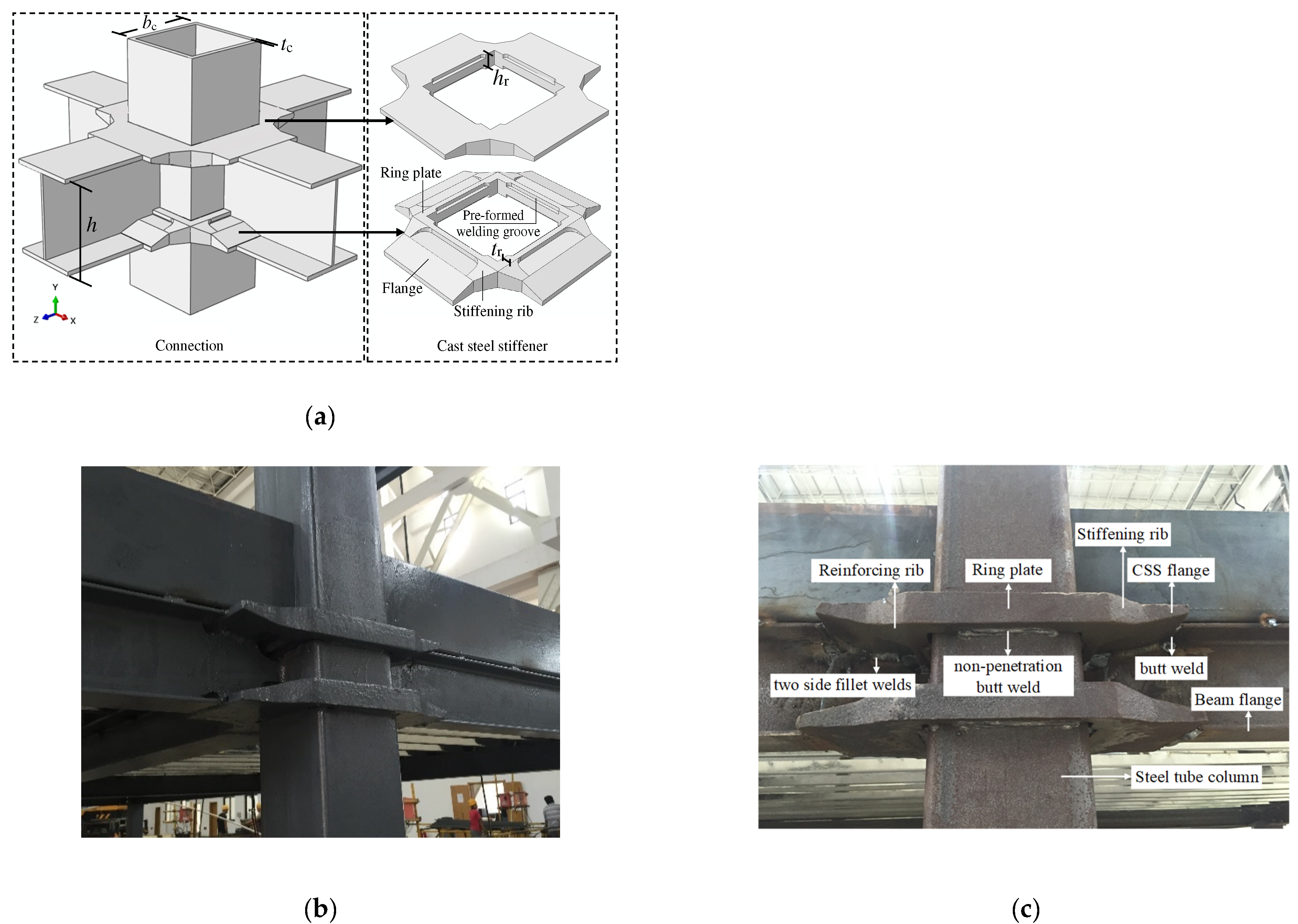
Figure 2.
Observations and predictions from the simplified theoretical model using Equation (1).

Figure 3.
Moment bearing capacity of Joints 1–5 without concrete.
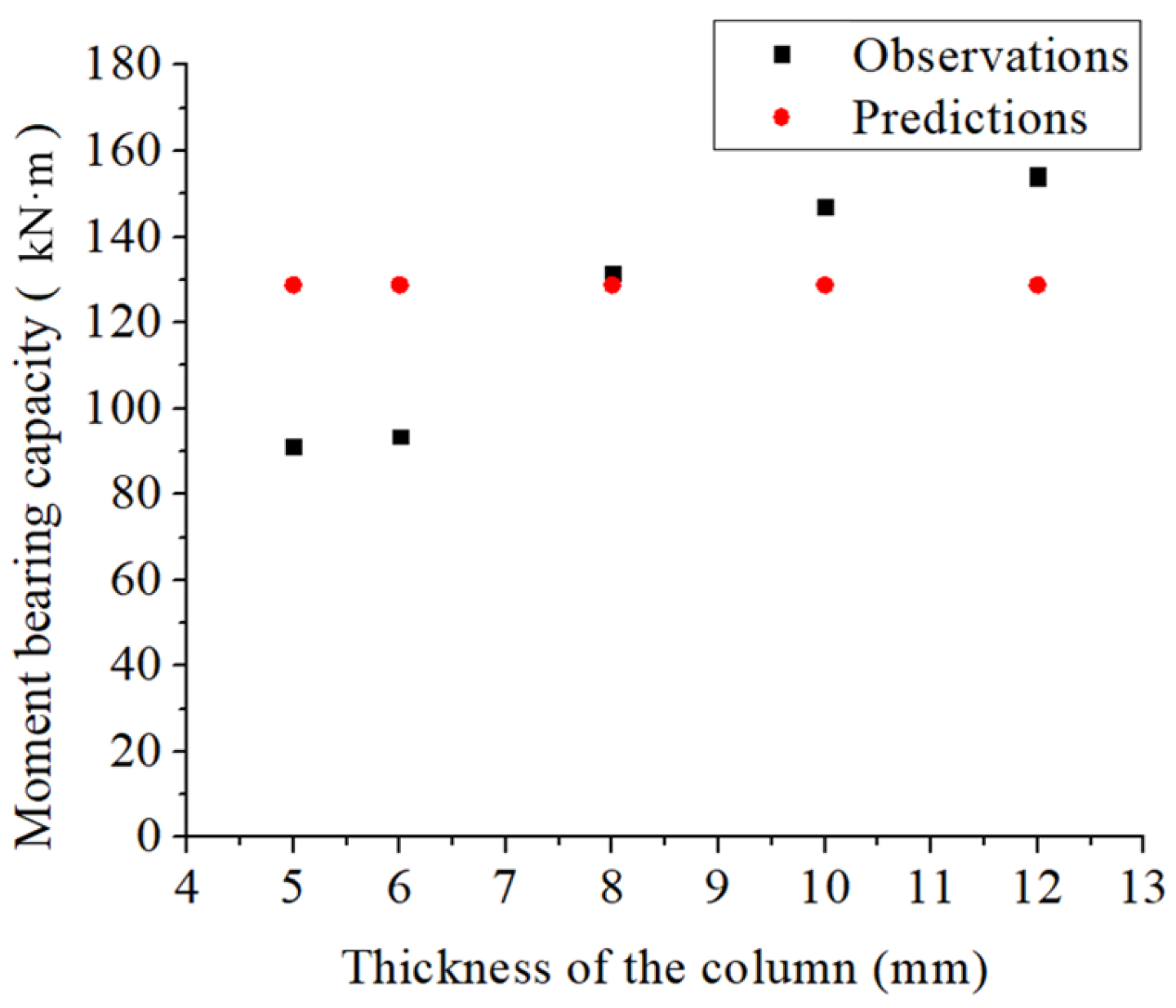
Figure 4.
Moment bearing capacity of Joints 38–41 with concrete filled in the column.

Figure 5.
Damage mechanism diagrams: (a) joint with thin wall column without concrete filled inside; (b) joint with thick wall column filled with concrete.
Figure 5.
Damage mechanism diagrams: (a) joint with thin wall column without concrete filled inside; (b) joint with thick wall column filled with concrete.

Figure 6.
Flowchart of the permutation-based feature variable importance analysis.

Figure 7.
A typical fragility curve conditional on .
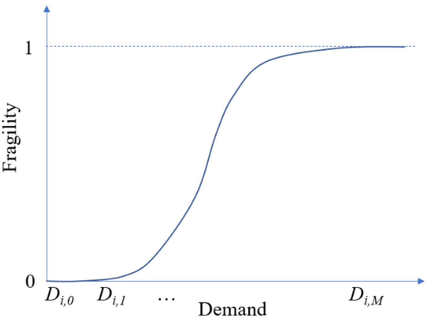
Figure 8.
Relationship between the observations and predictions from the proposed probabilistic model.
Figure 8.
Relationship between the observations and predictions from the proposed probabilistic model.

Figure 9.
Importance scores of feature variables.

Figure 10.
Fragility curves of Group 1.
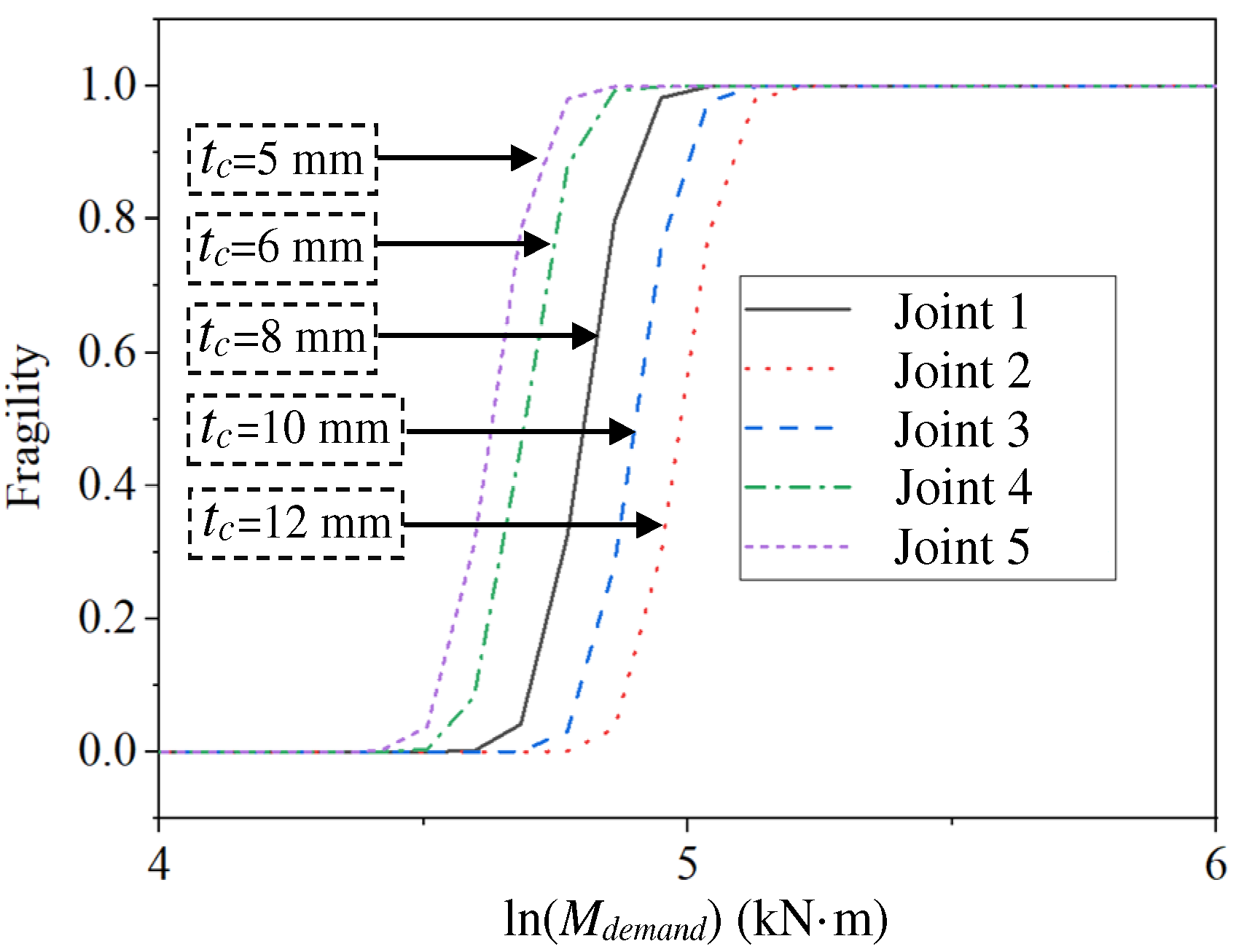
Figure 11.
Fragility curves of Group 2.
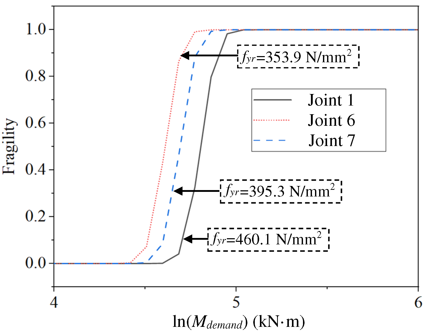
Figure 12.
Fragility curves of Group 3.

Figure 13.
Fragility curves of Group 4.

Figure 14.
Fragility curves of Group 5.
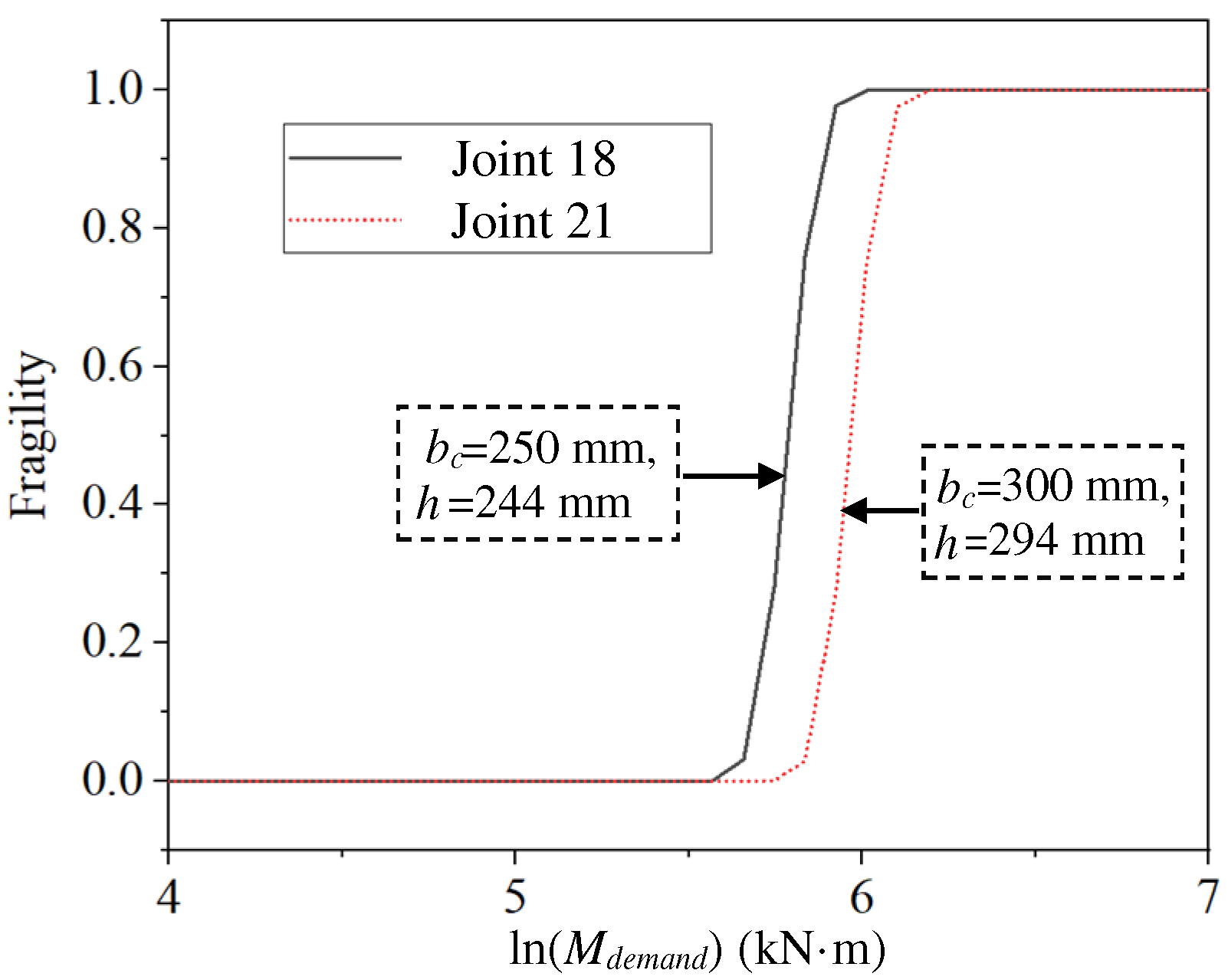
Figure 15.
Fragility curves of example joints with and without concrete filling.


Table 1.
Profiles of the 57 beam-column joints with CSS in the database, adapted from [5].
Table 1.
Profiles of the 57 beam-column joints with CSS in the database, adapted from [5].
| Joint | bc (mm) | tc (mm) | h (mm) | tr (mm) | hr (mm) | fyr (N/mm2) | fc (N/mm2) | Ma (kN·m) |
|---|---|---|---|---|---|---|---|---|
| 1 | 200 | 8 | 194 | 20 | 35 | 460.1 | - | 131.48 |
| 2 | 200 | 12 | 194 | 20 | 35 | 460.1 | - | 153.90 |
| 3 | 200 | 10 | 194 | 20 | 35 | 460.1 | - | 147.06 |
| 4 | 200 | 6 | 194 | 20 | 35 | 460.1 | - | 93.48 |
| 5 | 200 | 5 | 194 | 20 | 35 | 460.1 | - | 91.20 |
| 6 | 200 | 8 | 194 | 20 | 35 | 353.9 | - | 101.84 |
| 7 | 200 | 8 | 194 | 20 | 35 | 395.3 | - | 118.94 |
| 8 | 200 | 12 | 194 | 20 | 35 | 460.1 | - | 154.66 |
| 9 | 200 | 8 | 194 | 20 | 35 | 460.1 | 42.8 | 171.76 |
| 10 | 200 | 8 | 194 | 20 | 35 | 460.1 | 42.8 | 179.74 |
| 11 | 200 | 8 | 194 | 20 | 35 | 460.1 | 42.8 | 176.32 |
| 12 | 250 | 8 | 244 | 25 | 60 | 300.0 | - | 217.50 |
| 13 | 250 | 10 | 244 | 25 | 60 | 300.0 | - | 233.10 |
| 14 | 250 | 12 | 244 | 25 | 60 | 300.0 | - | 248.60 |
| 15 | 250 | 12 | 244 | 25 | 60 | 180.0 | - | 187.80 |
| 16 | 250 | 8 | 244 | 30 | 70 | 300.0 | - | 290.10 |
| 17 | 250 | 10 | 244 | 30 | 70 | 300.0 | - | 294.40 |
| 18 | 250 | 12 | 244 | 30 | 70 | 300.0 | - | 310.80 |
| 19 | 250 | 12 | 244 | 30 | 70 | 230.0 | - | 272.80 |
| 20 | 300 | 10 | 294 | 30 | 70 | 300.0 | - | 359.80 |
| 21 | 300 | 12 | 294 | 30 | 70 | 300.0 | - | 368.50 |
| 22 | 300 | 14 | 294 | 30 | 70 | 300.0 | - | 387.60 |
| 23 | 300 | 14 | 294 | 30 | 70 | 230.0 | - | 306.90 |
| 24 | 300 | 10 | 294 | 40 | 70 | 300.0 | - | 482.00 |
| 25 | 300 | 12 | 294 | 40 | 70 | 300.0 | - | 514.90 |
| 26 | 300 | 14 | 294 | 40 | 70 | 300.0 | - | 533.00 |
| 27 | 300 | 14 | 294 | 40 | 70 | 230.0 | - | 395.40 |
| 28 | 400 | 10 | 390 | 40 | 70 | 300.0 | - | 660.80 |
| 29 | 400 | 12 | 390 | 40 | 70 | 300.0 | - | 654.20 |
| 30 | 400 | 14 | 390 | 40 | 70 | 300.0 | - | 719.70 |
| 31 | 400 | 16 | 390 | 40 | 70 | 300.0 | - | 752.30 |
| 32 | 400 | 16 | 390 | 40 | 70 | 230.0 | - | 568.40 |
| 33 | 400 | 10 | 390 | 40 | 90 | 300.0 | - | 817.80 |
| 34 | 400 | 12 | 390 | 40 | 90 | 300.0 | - | 862.70 |
| 35 | 400 | 14 | 390 | 40 | 90 | 300.0 | - | 917.80 |
| 36 | 400 | 16 | 390 | 40 | 90 | 300.0 | - | 941.40 |
| 37 | 400 | 16 | 390 | 40 | 90 | 230.0 | - | 681.80 |
| 38 | 200 | 6 | 200 | 20 | 35 | 300.0 | 14.3 | 96.66 |
| 39 | 200 | 8 | 200 | 20 | 35 | 300.0 | 14.3 | 114.03 |
| 40 | 200 | 10 | 200 | 20 | 35 | 300.0 | 14.3 | 129.17 |
| 41 | 200 | 12 | 200 | 20 | 35 | 300.0 | 14.3 | 143.51 |
| 42 | 300 | 6 | 300 | 40 | 70 | 300.0 | 14.3 | 543.24 |
| 43 | 300 | 8 | 300 | 40 | 70 | 300.0 | 14.3 | 605.19 |
| 44 | 300 | 10 | 300 | 40 | 70 | 300.0 | 14.3 | 642.16 |
| 45 | 300 | 12 | 300 | 40 | 70 | 300.0 | 14.3 | 694.07 |
| 46 | 400 | 6 | 400 | 40 | 90 | 300.0 | 14.3 | 874.37 |
| 47 | 400 | 8 | 400 | 40 | 90 | 300.0 | 14.3 | 911.56 |
| 48 | 400 | 10 | 400 | 40 | 90 | 300.0 | 14.3 | 940.71 |
| 49 | 400 | 12 | 400 | 40 | 90 | 300.0 | 14.3 | 1025.83 |
| 50 | 500 | 6 | 500 | 50 | 100 | 300.0 | 14.3 | 1509.71 |
| 51 | 500 | 8 | 500 | 50 | 100 | 300.0 | 14.3 | 1566.02 |
| 52 | 500 | 10 | 500 | 50 | 100 | 300.0 | 14.3 | 1684.23 |
| 53 | 500 | 12 | 500 | 50 | 100 | 300.0 | 14.3 | 1704.18 |
| 54 | 600 | 6 | 600 | 50 | 100 | 300.0 | 14.3 | 1950.48 |
| 55 | 600 | 8 | 600 | 50 | 100 | 300.0 | 14.3 | 2175.25 |
| 56 | 600 | 10 | 600 | 50 | 100 | 300.0 | 14.3 | 2269.63 |
| 57 | 600 | 12 | 600 | 50 | 100 | 300.0 | 14.3 | 2332.84 |
Table 2.
Actual observational moment Ma and predicted moment Mp1 by using Equation (1).
| Joint | Ma (kN·m) | Mp1 (kN·m) | Absolute Prediction Error (%) | Joint | Ma (kN·m) | Mp1 (kN·m) | Absolute Prediction Error (%) |
|---|---|---|---|---|---|---|---|
| 1 | 131.48 | 128.83 | 2.02 | 30 | 719.70 | 655.20 | 8.96 |
| 2 | 153.90 | 128.83 | 16.29 | 31 | 752.30 | 655.20 | 12.91 |
| 3 | 147.06 | 128.83 | 12.40 | 32 | 568.40 | 502.30 | 11.63 |
| 4 | 93.48 | 128.83 | 37.82 | 33 | 817.80 | 842.40 | 3.01 |
| 5 | 91.20 | 128.83 | 41.26 | 34 | 862.70 | 842.40 | 2.35 |
| 6 | 101.84 | 99.09 | 2.70 | 35 | 917.80 | 842.40 | 8.22 |
| 7 | 118.94 | 110.68 | 6.94 | 36 | 941.40 | 842.40 | 10.52 |
| 8 | 154.66 | 128.83 | 16.70 | 37 | 681.80 | 645.80 | 5.28 |
| 9 | 171.76 | 128.83 | 24.99 | 38 | 96.66 | 84.00 | 13.10 |
| 10 | 179.74 | 128.83 | 28.32 | 39 | 114.03 | 84.00 | 26.34 |
| 11 | 176.32 | 128.83 | 26.93 | 40 | 129.17 | 84.00 | 34.97 |
| 12 | 217.50 | 219.60 | 0.97 | 41 | 143.51 | 84.00 | 41.47 |
| 13 | 233.10 | 219.60 | 5.79 | 42 | 543.24 | 504.00 | 7.22 |
| 14 | 248.60 | 219.60 | 11.67 | 43 | 605.19 | 504.00 | 16.72 |
| 15 | 187.80 | 168.40 | 10.33 | 44 | 642.16 | 504.00 | 21.51 |
| 16 | 290.10 | 307.40 | 5.96 | 45 | 694.07 | 504.00 | 27.38 |
| 17 | 294.40 | 307.40 | 4.42 | 46 | 874.37 | 864.00 | 1.19 |
| 18 | 310.80 | 307.40 | 1.09 | 47 | 911.56 | 864.00 | 5.22 |
| 19 | 272.80 | 235.70 | 13.60 | 48 | 940.71 | 864.00 | 8.15 |
| 20 | 359.80 | 370.40 | 2.95 | 49 | 1025.83 | 864.00 | 15.78 |
| 21 | 368.50 | 370.40 | 0.52 | 50 | 1509.71 | 1500.00 | 0.64 |
| 22 | 387.60 | 370.40 | 4.44 | 51 | 1566.02 | 1500.00 | 4.22 |
| 23 | 306.90 | 284.00 | 7.46 | 52 | 1684.23 | 1500.00 | 10.94 |
| 24 | 482.00 | 493.90 | 2.47 | 53 | 1704.18 | 1500.00 | 11.98 |
| 25 | 514.90 | 493.90 | 4.08 | 54 | 1950.48 | 1800.00 | 7.72 |
| 26 | 533.00 | 493.90 | 7.34 | 55 | 2175.25 | 1800.00 | 17.25 |
| 27 | 395.40 | 378.70 | 4.22 | 56 | 2269.63 | 1800.00 | 20.69 |
| 28 | 660.80 | 655.20 | 0.85 | 57 | 2332.84 | 1800.00 | 22.84 |
| 29 | 654.20 | 655.20 | 0.15 |
Table 3.
Posterior statistics of parameters in the probabilistic model.
| Parameter | Mean | Standard Deviation | Correlation Coefficient | ||||||||
|---|---|---|---|---|---|---|---|---|---|---|---|
| θ0 | θ1 | θ2 | θ3 | θ4 | θ5 | θ6 | θ7 | σ | |||
| θ0 | −10.950 | 0.533 | 1.000 | ||||||||
| θ1 | 0.594 | 0.094 | 0.208 | 1.000 | |||||||
| θ2 | 0.806 | 0.133 | −0.393 | −0.727 | 1.000 | ||||||
| θ3 | 0.948 | 0.103 | 0.252 | 0.087 | −0.404 | 1.000 | |||||
| θ4 | 0.753 | 0.088 | −0.263 | 0.130 | −0.299 | −0.559 | 1.000 | ||||
| θ5 | 0.747 | 0.066 | −0.795 | 0.199 | −0.203 | −0.024 | 0.426 | 1.000 | |||
| θ6 | 0.007 | 0.002 | 0.387 | 0.915 | −0.796 | 0.139 | 0.111 | 0.093 | 1.000 | ||
| θ7 | 4.547 | 0.382 | 0.045 | 0.200 | −0.190 | −0.103 | 0.268 | 0.006 | 0.058 | 1.000 | |
| σ | 0.069 | 0.007 | 0.009 | 0.019 | −0.022 | 0.010 | 0.002 | 0.005 | 0.022 | −0.014 | 1.000 |
Table 4.
Observations and predictions from the proposed probabilistic model for the moment capacity of CSS joints.
Table 4.
Observations and predictions from the proposed probabilistic model for the moment capacity of CSS joints.
| Joint | Ma (kN·m) | Mp (kN·m) | Absolute Prediction Error (%) | Confidence Interval | Joint | Ma (kN·m) | Mp (kN·m) | Absolute Prediction Error (%) | Confidence Interval |
|---|---|---|---|---|---|---|---|---|---|
| 1 | 131.48 | 121.92 | 7.27 | [122.71, 140.87] | 30 | 719.7 | 722.86 | 0.44 | [671.72, 771.11] |
| 2 | 153.9 | 146.34 | 4.91 | [143.64, 164.89] | 31 | 752.3 | 763.21 | 1.45 | [702.14, 806.04] |
| 3 | 147.06 | 134.42 | 8.60 | [137.26, 157.57] | 32 | 568.4 | 625.81 | 10.10 | [530.50, 609.00] |
| 4 | 93.48 | 108.95 | 16.55 | [87.25, 100.16] | 33 | 817.8 | 774.79 | 5.26 | [763.27, 876.22] |
| 5 | 91.2 | 102.43 | 12.31 | [85.12, 97.71] | 34 | 862.7 | 824.04 | 4.48 | [805.18, 924.33] |
| 6 | 101.84 | 100.22 | 1.59 | [95.05, 109.12] | 35 | 917.8 | 873.45 | 4.83 | [856.61, 983.36] |
| 7 | 118.94 | 108.85 | 8.48 | [111.01, 127.44] | 36 | 941.4 | 922.21 | 2.04 | [878.63, 1008.65] |
| 8 | 154.66 | 146.34 | 5.38 | [144.35, 165.71] | 37 | 681.8 | 756.19 | 10.91 | [636.34, 730.51] |
| 9 | 171.76 | 186.12 | 8.36 | [160.31, 184.03] | 38 | 96.66 | 100.75 | 4.23 | [90.22, 103.57] |
| 10 | 179.74 | 186.12 | 3.55 | [167.76, 192.58] | 39 | 114.03 | 112.76 | 1.11 | [106.43, 122.18] |
| 11 | 176.32 | 186.12 | 5.56 | [164.56, 188.92] | 40 | 129.17 | 124.31 | 3.76 | [120.56, 138.40] |
| 12 | 217.5 | 206.42 | 5.09 | [203.00, 233.04] | 41 | 143.51 | 135.33 | 5.70 | [133.94, 153.76] |
| 13 | 233.1 | 225.59 | 3.22 | [217.56, 249.75] | 42 | 543.24 | 510.40 | 6.05 | [507.02, 582.05] |
| 14 | 248.6 | 244.17 | 1.78 | [232.03, 266.36] | 43 | 605.19 | 554.78 | 8.33 | [564.84, 648.42] |
| 15 | 187.8 | 166.71 | 11.23 | [175.28, 201.22] | 44 | 642.16 | 601.02 | 6.41 | [599.35, 688.03] |
| 16 | 290.1 | 275.57 | 5.01 | [270.76, 310.82] | 45 | 694.07 | 646.73 | 6.82 | [647.79, 743.65] |
| 17 | 294.4 | 301.16 | 2.30 | [274.77, 315.43] | 46 | 874.37 | 873.91 | 0.05 | [816.07, 936.83] |
| 18 | 310.8 | 325.96 | 4.88 | [290.08, 333.00] | 47 | 911.56 | 922.59 | 1.21 | [850.78, 976.68] |
| 19 | 272.8 | 267.28 | 2.02 | [254.61, 292.29] | 48 | 940.71 | 982.14 | 4.40 | [877.99, 1007.91] |
| 20 | 359.8 | 362.45 | 0.74 | [335.81, 385.50] | 49 | 1025.83 | 1044.58 | 1.83 | [957.43, 1099.11] |
| 21 | 368.5 | 390.01 | 5.84 | [343.93, 394.82] | 50 | 1509.71 | 1572.42 | 4.15 | [1409.05, 1617.56] |
| 22 | 387.6 | 416.86 | 7.55 | [361.76, 415.29] | 51 | 1566.02 | 1612.30 | 2.96 | [1461.61, 1677.89] |
| 23 | 306.9 | 341.81 | 11.38 | [286.44, 328.82] | 52 | 1684.23 | 1686.59 | 0.14 | [1571.94, 1804.55] |
| 24 | 482 | 476.09 | 1.23 | [449.86, 516.43] | 53 | 1704.18 | 1773.01 | 4.04 | [1590.56, 1825.92] |
| 25 | 514.9 | 512.29 | 0.51 | [480.57, 551.68] | 54 | 1950.48 | 2046.71 | 4.93 | [1820.44, 2089.81] |
| 26 | 533 | 547.56 | 2.73 | [497.46, 571.08] | 55 | 2175.25 | 2038.30 | 6.30 | [2030.22, 2330.64] |
| 27 | 395.4 | 448.98 | 13.55 | [369.04, 423.65] | 56 | 2269.63 | 2095.23 | 7.68 | [2118.31, 2431.76] |
| 28 | 660.8 | 641.21 | 2.96 | [616.74, 708.01] | 57 | 2332.84 | 2177.03 | 6.68 | [2177.30, 2499.49] |
| 29 | 654.2 | 681.97 | 4.24 | [610.58, 700.93] |
Table 5.
The relationship between p%, Z, and γ.
| p% | Z | γ |
|---|---|---|
| 99 | 2.326 | 0.852 |
| 97.5 | 1.960 | 0.874 |
| 95 | 1.645 | 0.893 |
| 90 | 1.282 | 0.915 |
| 75 | 0.675 | 0.954 |
| 50 | 0 | 1 |
Table 6.
Joint grouping for the fragility curve comparison.
| Group ID | Joints in the Group | Logic |
|---|---|---|
| 1 | Joints 1 to 5 | Different column thicknesses (tc) |
| 2 | Joints 1, 6, and 7 | Different yield strengths of cast steel (fyr) |
| 3 | Joints 1 and 9 | Different axial compressive strengths of concrete (fc) |
| 4 | Joints 12 and 16 | Different heights and widths of the ring on the cast steel stiffener (hr and tr) |
| 5 | Joints 18 and 21 | Different outer diameters of the column and different distances between the outer surfaces of the upper and bottom flanges of the beam (bc and h) |
Table 7.
x of different joints.
| Joint | ln(tc) | ln(h) | ln(tr) | ln(hr) | ln(fyr) | bc/tc | fc/fyr |
|---|---|---|---|---|---|---|---|
| 1 | 2.079 | 5.268 | 2.996 | 3.555 | 6.131 | 25.000 | 0.000 |
| 2 | 2.485 | 5.268 | 2.996 | 3.555 | 6.131 | 16.667 | 0.000 |
| 3 | 2.303 | 5.268 | 2.996 | 3.555 | 6.131 | 20.000 | 0.000 |
| 4 | 1.792 | 5.268 | 2.996 | 3.555 | 6.131 | 33.333 | 0.000 |
| 5 | 1.609 | 5.268 | 2.996 | 3.555 | 6.131 | 40.000 | 0.000 |
| 6 | 2.079 | 5.268 | 2.996 | 3.555 | 5.869 | 25.000 | 0.000 |
| 7 | 2.079 | 5.268 | 2.996 | 3.555 | 5.980 | 25.000 | 0.000 |
| 9 | 2.079 | 5.268 | 2.996 | 3.555 | 6.131 | 25.000 | 0.093 |
| 12 | 2.079 | 5.497 | 3.219 | 4.094 | 5.704 | 31.250 | 0.000 |
| 16 | 2.079 | 5.497 | 3.401 | 4.248 | 5.704 | 31.250 | 0.000 |
| 18 | 2.485 | 5.497 | 3.401 | 4.248 | 5.704 | 20.833 | 0.000 |
| 21 | 2.485 | 5.684 | 3.401 | 4.248 | 5.704 | 25.000 | 0.000 |
Table 8.
Fragilities of different joints under varied ln(Mdemand).
| Joint | ln(Mdemand) | |||||||||||
|---|---|---|---|---|---|---|---|---|---|---|---|---|
| 4.329 | 4.506 | 4.684 | 4.861 | 5.038 | 5.215 | 5.392 | 5.570 | 5.747 | 5.924 | 6.101 | 6.278 | |
| 1 | 0.000 | 0.000 | 0.041 | 0.797 | 1.000 | 1.000 | 1.000 | 1.000 | 1.000 | 1.000 | 1.000 | 1.000 |
| 2 | 0.000 | 0.000 | 0.000 | 0.035 | 0.775 | 1.000 | 1.000 | 1.000 | 1.000 | 1.000 | 1.000 | 1.000 |
| 3 | 0.000 | 0.000 | 0.001 | 0.281 | 0.977 | 1.000 | 1.000 | 1.000 | 1.000 | 1.000 | 1.000 | 1.000 |
| 4 | 0.000 | 0.004 | 0.458 | 0.993 | 1.000 | 1.000 | 1.000 | 1.000 | 1.000 | 1.000 | 1.000 | 1.000 |
| 5 | 0.000 | 0.038 | 0.785 | 1.000 | 1.000 | 1.000 | 1.000 | 1.000 | 1.000 | 1.000 | 1.000 | 1.000 |
| 6 | 0.000 | 0.072 | 0.866 | 1.000 | 1.000 | 1.000 | 1.000 | 1.000 | 1.000 | 1.000 | 1.000 | 1.000 |
| 7 | 0.000 | 0.004 | 0.463 | 0.993 | 1.000 | 1.000 | 1.000 | 1.000 | 1.000 | 1.000 | 1.000 | 1.000 |
| 9 | 0.000 | 0.000 | 0.000 | 0.000 | 0.003 | 0.436 | 0.992 | 1.000 | 1.000 | 1.000 | 1.000 | 1.000 |
| 12 | 0.000 | 0.000 | 0.000 | 0.000 | 0.000 | 0.048 | 0.818 | 1.000 | 1.000 | 1.000 | 1.000 | 1.000 |
| 16 | 0.000 | 0.000 | 0.000 | 0.000 | 0.000 | 0.000 | 0.001 | 0.238 | 0.968 | 1.000 | 1.000 | 1.000 |
| 18 | 0.000 | 0.000 | 0.000 | 0.000 | 0.000 | 0.000 | 0.000 | 0.001 | 0.282 | 0.977 | 1.000 | 1.000 |
| 21 | 0.000 | 0.000 | 0.000 | 0.000 | 0.000 | 0.000 | 0.000 | 0.000 | 0.001 | 0.271 | 0.975 | 1.000 |
Publisher’s Note: MDPI stays neutral with regard to jurisdictional claims in published maps and institutional affiliations. |
© 2022 by the authors. Licensee MDPI, Basel, Switzerland. This article is an open access article distributed under the terms and conditions of the Creative Commons Attribution (CC BY) license (https://creativecommons.org/licenses/by/4.0/).
Share and Cite
MDPI and ACS Style
Li, X.; Xu, H. Probabilistic Moment Bearing Capacity Model and Fragility of Beam-Column Joints with Cast Steel Stiffeners. Buildings 2022, 12, 577. https://doi.org/10.3390/buildings12050577
AMA Style
Li X, Xu H. Probabilistic Moment Bearing Capacity Model and Fragility of Beam-Column Joints with Cast Steel Stiffeners. Buildings. 2022; 12(5):577. https://doi.org/10.3390/buildings12050577
Chicago/Turabian StyleLi, Xinxia, and Hao Xu. 2022. "Probabilistic Moment Bearing Capacity Model and Fragility of Beam-Column Joints with Cast Steel Stiffeners" Buildings 12, no. 5: 577. https://doi.org/10.3390/buildings12050577
Note that from the first issue of 2016, this journal uses article numbers instead of page numbers. See further details here.