
The Spatiotemporal Distribution Characteristics and Driving Factors of Carbon Emissions in the Chinese Construction Industry

1
College of Civil Engineering, Sanjiang University, Nanjing 210012, China
2
College of Civil Engineering, Nanjing Forestry University, Nanjing 210037, China
*
Author to whom correspondence should be addressed.
Buildings 2023, 13(11), 2808; https://doi.org/10.3390/buildings13112808
Submission received: 30 September 2023
/
Revised: 5 November 2023
/
Accepted: 7 November 2023
/
Published: 9 November 2023
(This article belongs to the Special Issue Green Building Design and Construction for a Sustainable Future)
Abstract
:As a pillar industry of the national economy, the construction industry not only promotes urban development and social prosperity but also has an irreversible impact on the environment with the trend of high carbon emissions. Therefore, it is of great significance for the construction industry to take the lead in achieving carbon emissions reduction. This paper attempts to explore the spatiotemporal distribution characteristics and specific driving factors of carbon emissions in the construction industry in 30 provinces of China from 2011 to 2020 based on the spatial econometric analysis, so as to clarify the development trajectory and formation mechanism. The key findings are (1) there are obvious differences in carbon emissions across Chinese provinces, culminating in a distinct “Belt–Ring–Dot” spatial distribution; (2) the carbon emissions in the construction industry follow an inverted U-shaped pattern from south to north, with lower emissions in the west and higher emissions in the east, which means the pressure and potential of carbon emissions reduction coexist; (3) the Moran’s I index values from 2011 to 2020 were all greater than 0, with a maximum value of 0.284, indicating that there is a notable positive spatial correlation in carbon emissions in the construction industry between provinces; and (4) among the five factors, the number of employees displays the most pronounced spatial correlation, passing the test a total of eight times, and the mean test coefficient is the largest at 0.552. This factor positively influences carbon emissions alongside the gross product. On the other hand, the patents granted factor significantly inhibits carbon emissions with all test coefficients being negative with a maximum absolute value of 0.166. The impact of the technical equipment rate shows a characteristic of initial positive stimulation followed by later negative inhibition. In contrast, the urbanization rate exhibits the weakest spatial correlation with the minimum test coefficient being only 0.001.
1. Introduction
On 15 November 2022, the World Meteorological Organization (WMO) released an interim report on “Global Climate Conditions 2022”, which stated that the global average temperature in 2022 was about 1.15 °C higher than the pre-industrial period (1850–1900), and the last eight years may have been the hottest years on record. Since most of the greenhouse gases that cause climate warming are carbon dioxide, reducing carbon emissions can mitigate the severe risks and adverse effects of climate change to the greatest extent [1]. The UK was the world’s largest carbon emitter from the Industrial Revolution until it was replaced by the US in 1888. Since then, developing countries have relied on fossil energy to accelerate urban development, resulting in a rapid increase in carbon emissions. By 2006, China had surpassed the US to become the country with the largest carbon emissions in the world [2]. The Chinese government put forward the “Dual Carbon Targets” at the 75th session of the United Nations General Assembly in this grim situation, aiming to solve the dilemma of resource and environmental constraints and achieve green sustainable development [3].
Recent studies suggest that the construction industry globally is responsible for approximately one-quarter of carbon emissions [4]. The reason is that compared to other sectors, the construction industry is a resource-intensive industry that consumes a large amount of fossil energy, thereby increasing carbon emissions while promoting the rapid development of urbanization, and improving people‘s livelihoods [5]. Therefore, it is of great significance for the construction industry to take the lead in achieving carbon emissions reduction. However, the achievement of emission reduction targets depends not only on national policies but also on provincial actions [6]. In particular, China is in the development stage, and the development level of the construction industry varies between different regions, as well as between resource endowment and technological levels. Meanwhile, the existing research predominantly concentrates on carbon emissions within a specific region, or explores them from a single perspective of time or space, ignoring the evolution characteristics across different regions. How to clarify the different characteristics of carbon emissions in the construction industry for the implementation of differentiated carbon reduction measures is worth careful consideration.
It has also been found that there may be significant carbon emission interactions between provinces, which means the mechanisms affect both local and neighboring regions [7]. Therefore, by using the carbon emissions data of the construction industry in 30 provinces from 2011 to 2020, this paper attempts to explore the spatiotemporal distribution characteristics and formation mechanisms of carbon emissions from the construction industry at the provincial level in China, based on spatial econometric analysis. And it exhibits innovation in three aspects. Firstly, it delves into the dynamic evolution characteristics of carbon emissions in the construction industry by integrating a dual perspective of time and space, presenting them visually. Secondly, it validates the spatial correlation of carbon emissions in the construction industry and unveils new distribution patterns through the Moran’s index. Finally, the inclusion of technological innovation factors in the spatial econometric model adds a crucial dimension and has significantly enriched the research findings. It is expected to provide a scientific basis for the relevant government departments to formulate differentiated carbon emission reduction measures and the overall linkage governance program in the construction industry.
This paper is structured as follows. Section 2 reviews the existing literature on the carbon emission. Section 3 presents the data sources and research methods. Section 4 presents the results of the spatial econometric analysis. Section 5 discusses the results. Finally, the conclusions are presented in Section 6.
2. Literature Review
2.1. Carbon Emissions Distribution
According to the existing literature collection, the distribution characteristics of carbon emissions are analyzed in different countries and regions or different industrial sectors. For example, Yang et al. (2018) observed that the spatial distribution of total carbon emissions in China primarily exhibits a pattern of higher levels in the east and lower levels in the west [8]. Building upon this observation, Liu et al. (2021) identified a specific trend characterized by the central agglomeration in the northeast–southwest direction and spatial divergence in the northeast–southeast direction [9]. Gregg et al. (2009) explored that the characteristics of fossil-fuel-based carbon emissions on a monthly scale have greater temporal and spatial variability than the flux aggregated to the national annual level in North America [10]. At the global level, some scholars have found that there is cross-country convergence in carbon emissions [11], while with the passage of time and economic development, other scholars hold the opposite view [12]. These viewpoints collectively indicate spatial variations in the distribution of carbon emissions. From the perspective of different industrial sectors, the aforementioned studies on carbon emissions have broadly encompassed various sectors, including industry, transportation, and construction [13]. Some scholars have also focused their attention on agriculture, aviation, logistics, and so on [14]. For instance, Zhou et al. (2022) found that the carbon emissions of agriculture are basically characterized by rapid growth in the early stage and gradual stabilization in the later stage [15]. Liu et al. (2019), focusing on local carbon emissions from civil airports, discovered that the emission intensity in the central and eastern regions of China is significantly higher than that in the northeast and western regions [16]. At present, the construction industry is known as a representative industry for its high energy consumption and pollution where the spatial distribution of emission efficiency is unbalanced [17], contributing to regional disparities with an increasing trend of international linkage effects [18]. Meanwhile, some scholars have attempted to explore the variation characteristics of carbon emissions during the operational phase of buildings from a life cycle perspective [19].
2.2. Influencing Factors
On account of the complex system formed by the interaction of various factors [8], it is necessary to correctly identify the impact mechanism of carbon emissions in order to establish an effective reduction strategy as soon as possible. Generally speaking, the driving force behind carbon emissions cannot be separated from overall factors such as economic level, scientific and technological capabilities, population, and policy guidance of a country or region [20]. Among them, industrial structure, per capita income, population, and urbanization level have a positive driving effect on carbon emissions [21], while scientific and technological capabilities and policy releases have a negative inhibitory effect [22]. However, it is worth noting that the impact of economic level and industrial structure is not simple, as studies have found variations in their influence [23]. For instance, there is no consensus on whether trade openness has a positive impact on decoupling carbon emissions from economic growth in high-income countries [24], while there is consensus that it has a more negative impact on low-income countries [25]. As for industrial agglomeration, Gong et al. (2022) found that the agglomeration of primary and secondary industries in China promotes carbon emissions while the agglomeration of tertiary industries has a significant effect on reduction [26]. Despite the varying characteristics of carbon emission factors in different industrial sectors and regions, the construction industry is resource-intensive and involves all aspects of urban production, consumption, and circulation, which are necessary to clarify the individual factors consistent with its characteristics [27]. Some studies have been conducted to investigate whether the structure of the construction industry, output scale effect [28], land expansion, and building materials are the main factors of carbon emissions [29]. Conversely, energy intensity, green building, low-carbon construction patents, and policies have negative effects [30]. For example, Hou (2021) argues that mechanisms to reform supply-side incentives could offer immediate benefits [31].
2.3. Relevant Research Methods
For the measurement of carbon emissions data, the most widely accepted and used by countries around the world is the Intergovernmental Panel on Climate Change (IPCC) Sectoral Approach, which provides a standardized approach for countries to estimate their greenhouse gas emissions and removal [32]. Regarding the distribution of carbon emissions, Liu et al. (2022) conducted a comparative analysis of the basic data of industrial carbon emissions to explore its development trend in Jiangsu Province [33]. In addition, some researchers predicted carbon emissions by modifying the Moon–Sonn model or using the gray model GM (1, 1) [34]. Liu et al. (2022) conducted a peak analysis of agricultural carbon emissions in Shandong Province using the Moon–Sonn model [35]. Recently, more researchers have discovered that the spatial relationships between cities are becoming stronger, making the connections of carbon emissions more intricate and extensive. To better analyze these spatial effects, scholars have started using methods such as social network analysis and spatial econometrics [36]. For example, Zheng et al. (2022) combined Social Network Analysis (SNA) with Quadratic Assignment Procedure (QAP) to measure the spatial correlation network characteristics of carbon emissions in the Pearl River Delta urban agglomeration in China [37]. Wang et al. (2022) calculated the Moran’s I index of carbon emissions from the construction industry by spatial exploration methods at both global and Chinese scales, revealing a significant positive autocorrelation across diverse urban areas [38]. In the realm of carbon emissions impact analysis, a rich array of existing methods has been employed. Most researchers have collected panel data and employed the Kaya Identity to decompose the driving factors of carbon emissions. Subsequently, they use the Logarithmic Mean Divisia Index (LMDI) model to disaggregate the contributions of each factor [26]. Additionally, some scholars have utilized various methods including Panel Vector Auto-Regressive (PVAR) models [39], Stochastic Impacts by Regression on Population, Affluence, and Technology (STIRPAT) models [40], Random Forest models [41], Granger causality tests [42], and system dynamics to identify and analyze the influencing factors of carbon emissions [43]. In contrast, a minority of scholars have adopted a spatial econometrics perspective by incorporating spatial weight matrices into their analyses [44]. They have employed Spatial Error, Lag, and Durbin models to investigate the factors while accounting for spatial dependencies [45].
2.4. Literature Summary
In summary, extant literature exhibits diversities in research perspectives, content, and methodologies concerning carbon emissions. Nevertheless, it predominantly concentrates on the assessment of carbon emissions distribution within individual national or provincial regions, thereby disregarding potential spatial interactions with adjacent areas. Furthermore, prevalent approaches primarily encompass measurements conducted along either temporal or spatial dimensions, thus failing to capture the nuanced spatiotemporal dynamics inherent in simultaneous processes influencing carbon emissions distribution. Therefore, to address the deficiencies in the existing research, this study utilizes exploratory spatial statistical analysis to examine the spatiotemporal trends of carbon emissions in the construction industry across Chinese provinces from 2010 to 2020. Additionally, spatial econometric models are employed to investigate the driving factors contributing to regional disparities. The objective is to furnish a theoretical foundation and policy implications for China’s carbon reduction initiatives, facilitating the realization of environmentally friendly and low-carbon development within the construction industry.
3. Data and Methods
This study integrates the IPCC Sectoral Approach, provincial greenhouse gas inventory guidelines, and the Chinese carbon accounting database to calculate carbon emissions from the construction industry in 30 provinces of China from 2010 to 2020, so as to conduct descriptive statistical analyses [46]. Subsequently, we attribute spatial characteristics to the dataset, exploring its spatiotemporal distribution patterns and developmental trends. Conclusively, the approach involves the meticulous selection of influential factors from multifaceted vantage points encompassing economic, social, demographic, technological, and innovation dimensions. These selected factors form the basis for the construction of a spatial econometric model, employed to probe the intricate causal mechanisms that underlie the observed phenomena.
3.1. Data Definition and Source
3.1.1. Vector Data of Carbon Emissions
The research subject of this study is the carbon dioxide emissions from the construction industry in 30 provinces across China (excluding Hong Kong, Taiwan, Tibet, and Macao) from 2011 to 2020. This dataset not only includes the specific annual emissions values for the construction industry but also encompasses the geographical coordinates of these 30 provinces, representing a vector dataset that combines both economic and spatial attributes. The spatial attribute data consist of coordinates for administrative regions of 30 provinces in China and originate from the Resource and Environment Science and Data Center. The economic attribute data represent the carbon emissions for each province in the construction industry. To derive carbon emissions data, this study combines the IPCC Sectoral Approach, provincial greenhouse gas inventory guidelines, and the Chinese carbon accounting database. Specifically, based on the physical quantity data extracted from the provincial energy balance tables found in the China Energy Statistical Yearbook, we consider 17 categories of fossil fuel energy consumption within the construction industry including raw coal, coke, crude oil, gasoline, kerosene, diesel, fuel oil, petroleum asphalt, liquefied petroleum gas, natural gas, and others. Then Equation (1) is used to measure the carbon emissions:
where is the consumption of the nth fossil energy, is average low calorific value of the nth fossil energy, and is carbon content per unit calorific value of the nth fossil energy.
3.1.2. Factors Selection
The relationship between economic activities and the environment can be decomposed into scale, structure, and technological effects [47]. Considering that previous literature has extensively explored mature factors affecting carbon emissions, such as economic levels, industrial structure, energy intensity, and material consumption [21], and recognizing that decarbonization in the construction industry is closely tied to the development of green building and technological innovation, this paper endeavors to select factors related to carbon emissions from the perspectives of machinery utilization and technological innovation. In view of the availability of data, the rate of technical equipment and the number of granted patents in the construction industry are characterized. The rate of technological equipment refers to the ratio of the net value of self-owned mechanical equipment to the total number of workers of construction industry enterprises at the end of the year, reflecting the level of mechanization and technological investment. The number of granted patents represents the count of invention patents authorized by the intellectual property administrative department, indicating the level of scientific development and innovation capability in each province. Given the diversity and comprehensiveness of influencing factors, this study incorporates three influencing factors from the perspectives of economic, social, and population development, including gross product of construction industry, provincial urbanization rates, and the number of employees in the construction industry. The definitions of the variables are shown in Table 1. The aforementioned original data are sourced from annual publications such as China Statistical Yearbook, China Construction Industry Statistical Yearbook, China Energy Statistical Yearbook, and China Science and Technology Statistical Yearbook.
3.2. Spatial Econometric Analysis
3.2.1. Spatial Correlation Analysis
American geographer W.R. Tobler proposed that everything is related to everything else, but near things are more related than distant things in 1970 [48]. This principle is known as the First Law of Geography, which means that different phenomena are more similar when they are closer in space, indicating the presence of spatial correlation. If the opposite is observed, meaning that closer objects are less similar, it indicates spatial heterogeneity. When there is no relationship between the attributes of objects and their spatial positions, it suggests that the attribute lacks spatial correlation [49]. Therefore, whether there exists spatial correlation among various economic variables at different distances in different regions needs to be statistically measured. The Moran’s I index, proposed by Australian statistician Patrick Alfred Pierce Moran in 1950, is a widely used metric in global spatial autocorrelation analysis of economic variables to measure the degree of spatial correlation and regional homogeneity. Its definition is as follows:
where n represents the number of provinces in China, and represent carbon emissions in provinces i and j, c is the average carbon emissions in all provinces, and is the spatial weight matrix and represents the spatial disparity between regions i and j.
is a binary spatial weight matrix, which can be categorized into two types. One is based on adjacency, where regions share common boundaries, and the other is based on distance, where the distance between the centroids of regions is less than a given critical value. The selection of the spatial weight matrix can affect the calculation of the ratio. In this paper, since the regions are represented by provincial surface data and provinces share common boundaries with each other, we have chosen the spatial weight matrix based on adjacency. Its form is as follows:
The Moran’s I index typically ranges between [−1 and 1]. When Moran’s I > 0, it indicates a positive spatial correlation in the carbon emissions from the construction industry among different regions, meaning that neighboring regions have similar emissions. When Moran’s I < 0, it indicates a negative spatial correlation, signifying those emissions are heterogeneous among neighboring regions. When Moran’s I = 0, it suggests that there is no spatial correlation, implying that emissions are independent of each region [50].
3.2.2. Spatial Econometric Models
The two fundamental types of spatial econometric models can be classified based on the way spatial dependencies are introduced. One is the introduction of spatial lag correlation, known as the Spatial Lag Model (SLM); the other introduces spatial error dependence, referred to as the Spatial Error Model (SEM). The former involves correlation in the dependent variable, while the latter involves correlation in the error terms. These models are used in spatial econometrics to handle spatial dependencies and better capture the relationships between observations in spatial datasets [51].
- Spatial Lag Model (SLM)
The SLM examines whether various variables in a particular region exhibit diffusion or spillover effects. The dependent variable is influenced not only by the independent variables within the same region but also by the dependent variables in neighboring regions. The expression for this model is as follows:
where y is the dependent variable, X is the matrix of explanatory variables, W is the spatial weight matrix, is the spatial autoregressive coefficient, is the parameter vector, and is the error term. This relationship reflects the spatial dependency in the sample observations, indicating how the observations in neighboring regions influence the observations in the focal region, including both the direction and magnitude of the influence.
- Spatial Error Model (SEM)
The SEM is used to capture the spatial interactions between individual units by considering spatial correlations within the error term. This model is applicable when there are variations in the spatial interactions among units due to differences in their relative positions. The expression for SEM is as follows:
where is the spatial error term in the cross-sectional dependent variable vector, denotes independently distributed random error terms that measure the spatial dependency effects present in the error disturbances and also quantify the extent to which neighboring areas affect the observed values in the local area due to errors in the dependent variable.
4. Results
4.1. Initial Exploration of Carbon Emissions
4.1.1. Statistics of the Carbon Emissions
From the Table 2, the annual carbon emission values are valid and there are no default data. It can be observed that although the average carbon emissions from the construction industry in each province generally exhibit an upward trend, the median values exhibit a fluctuating decline. They reach their troughs in 2011, 2015, and 2018, and peak in 2013, 2016, and 2019. Simultaneously, the peak values are decreasing, indicating a declining trend in carbon emissions for provinces located around the dataset’s median values. It reflects that these provinces have implemented carbon emission reduction measures and achieved certain results during this period. The increase in the average, on the other hand, may be attributed to the influence of extreme values in certain provinces. Especially when examining the percentile values, half of the provinces have carbon emissions of only 2 million tons, significantly lower than the maximum value of 6 million tons. Additionally, the carbon emissions of three-quarters of the provinces are also around 3 million tons, with only half of the maximum value. The difference between the minimum and maximum values is significant. By this token, the carbon emissions of most provinces are relatively close to each other, while a small number of provinces exhibit significant differences in carbon emissions, indicating a greater pressure for emissions reduction in those areas.
4.1.2. Carbon Emissions Trends
According to Figure 1, on the one hand, there are 4 provinces out of the 30 provinces in China that have cumulatively emitted more than 40 million tons of carbon in the construction industry from 2011 to 2020. These provinces are Jiangsu, Zhejiang, Hubei, and Hunan, with Zhejiang having the highest emissions at 53.80 million tons. On the other hand, there are three provinces with emissions totaling less than 5 million tons, which are Guangxi, Hainan, and Heilongjiang. Among them, Heilongjiang has the lowest carbon emissions, amounting to only 2.74 million tons, approximately 4% of Zhejiang’s emissions. Over the course of a decade, the carbon emissions in several provinces exhibit different trends. Shanghai, Beijing, Shandong, Hubei, Liaoning, and Shanxi, consistently witness year-to-year reductions in carbon emissions. Conversely, provinces like Jilin, Hebei, and Shaanxi initially experienced an increase in emissions followed by a subsequent decrease. Anhui, Jiangxi, Ningxia, Henan, Guizhou, and Hunan register slight increases in emissions. Meanwhile, areas like Yunnan, Tianjin, Jiangsu, Fujian, and Chongqing maintain relatively stable emission levels.
From this perspective, carbon emissions in the 30 provinces of China vary significantly. Although the construction industry has made some progress in reducing carbon emissions since the introduction of energy-saving and emission reduction targets during the “Eleventh Five-Year Plan” and the subsequent issuance of several guiding documents, the carbon emissions in some provinces remain high. This is due to the crucial role of the construction industry in the economic development and urbanization of developing countries. Hence, high carbon emission areas must simultaneously address the challenges and capitalize on opportunities for further carbon reduction. This also indirectly shows that there are regional disparities in the management of carbon emissions, which will help us gain an in-depth understanding of the diverse performances and challenges in carbon reduction across different areas.
4.2. Spatiotemporal Distribution Characteristics of Carbon Emissions
4.2.1. Spatiotemporal Distribution Pattern
From Figure 2, it is evident that there is a significant regional disparity in carbon emissions. Beginning in 2010, the northern region, including Inner Mongolia, the central region, with Hubei, and the eastern coastal areas such as Shandong and Zhejiang, exhibited the highest emissions. In contrast, the northeastern province of Heilongjiang, northwestern Qinghai, and southern Guangxi had the lowest carbon emissions during this period. However, emissions in Inner Mongolia and Sichuan began to decrease annually, while, from 2012, the central region’s emissions gradually increased and formed a central cluster. This cluster encompassed provinces such as Hunan, Hubei, Henan, Anhui, Zhejiang, Jiangsu, and Guangdong, forming a roughly circular distribution around the lower-emission area of Jiangxi. By 2015, the circular distribution pattern became more pronounced, along with southwestern Sichuan, collectively radiating toward the central region. Emissions began to decrease in most areas to the north along the line from the westernmost Xinjiang to the easternmost Heilongjiang. In contrast, emissions in the central regions of Henan and Hunan, as well as in the western regions of Sichuan and Yunnan, showed a gradual increase. Meanwhile, the eastern coastal areas, including Shandong, Zhejiang, and Jiangsu, consistently remained in the high emissions zone. By 2020, it had developed into a transverse low-value distribution belt spanning from east to west (referred to as the “Belt”). This belt separated the high-value regions of northern Inner Mongolia from the eastern coastal areas, including Zhejiang, Jiangsu, and Shandong, in addition to the central regions of Henan, Hunan, and Sichuan (referred to as the “Ring” and the “Dot”). Ultimately, this pattern evolved into the “Belt–Ring–Dot” spatial distribution, exhibiting a noticeable spatial clustering characteristic.
This distribution pattern indicates that, on a national scale, carbon emissions from the construction industry exhibit a specific clustering pattern in space, which is differentiated and uneven. The “Belt” represents a low-value aggregation area of carbon emissions horizontally, while the “Ring” and the “Dot” are high-value aggregation areas. This spatial clustering property suggests that carbon emissions from the construction industry are not only influenced by local factors such as economic development, industrial structure, and energy consumption, but also by the influence of neighboring regions. Therefore, in the study of influencing factors on carbon emissions from the construction industry, it is necessary to consider the existence of spatial clustering effects.
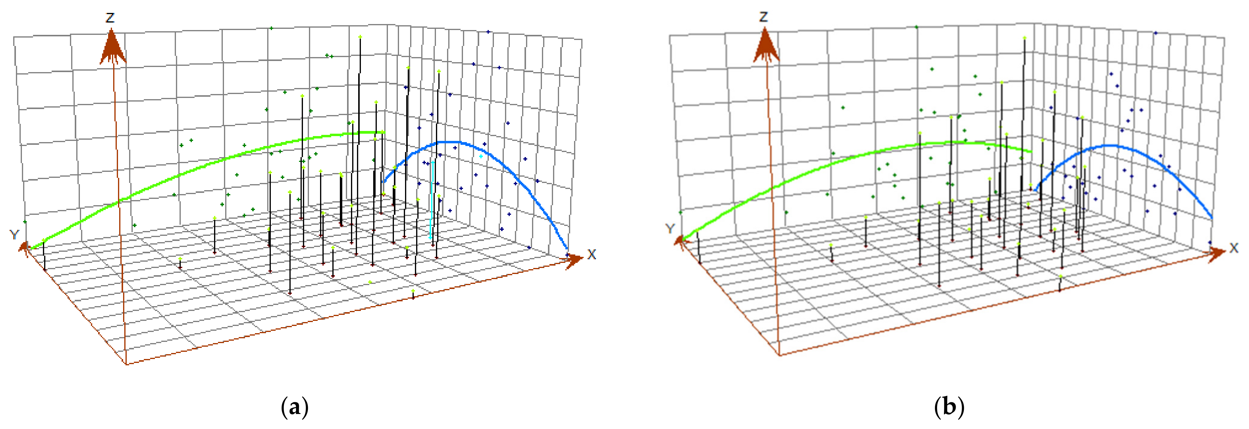
The Y-axis in the trend analysis graph represents the north–south direction, the X-axis represents the east–west direction, and the Z-axis represents carbon emissions. The blue line connects the projected points of carbon emissions in the north–south direction, while the green line represents the east–west direction. This line signifies the simulated optimal trend direction for carbon emissions in the construction industry. Connecting the projected points with lines allows us to simulate the most suitable trend direction. Upon examination, it becomes apparent that the spatial trends in carbon emissions in the construction industry are relatively consistent across provinces, thus warranting our focus on presenting the trend analysis only for 2011 and 2020. Figure 3 illustrates that there is a clear inverted U-shaped trend in the north–south direction, while in the east–west direction, emissions are lower in the west and higher in the east. This suggests that the central regions of China exhibit higher carbon emissions, gradually decreasing toward the north and south, while the western regions demonstrate lower emissions compared to the eastern regions. This aligns with the spatial distribution of carbon emissions in Figure 2. Furthermore, the trend analysis graph also indicates that as carbon emissions move eastward, the rate of increase in carbon emissions slows down, and after reaching a peak, there is a slight decreasing trend. From this observation, it becomes evident that there exists a substantial spatial disparity in carbon emissions from the construction industry among provinces in China.
4.2.2. Global Spatial Autocorrelation Analysis
To verify the spatial effects of carbon emissions in the provincial-level construction industry in China, a spatial weight matrix based on adjacency relationships is constructed. Since Hainan Province is an independent island and does not share a land border with other provinces and cities, the calculation index will be excluded. Therefore, for the sake of data completeness and accuracy, we adjusted the adjacency of Hainan Province with Guangdong Province and Guangxi Province. The final calculation results are as Table 3.
From 2011 to 2020, the Moran’s I index values of carbon emissions were all greater than 0, with a minimum value of 0.124 in 2010 and increasing fluctuation thereafter, reaching a maximum of 0.284 in 2018. Additionally, the p-value passed the 5% significance test in the first two years, while the p-value consistently passed the 1% significance test in the last eight years. This demonstrates that there is a certain positive spatial correlation in carbon emissions in the construction industry. Specifically, when the carbon emissions in one region’s construction industry are high, the surrounding or adjacent regions also tend to exhibit elevated carbon emissions in a spatially consistent pattern. Meanwhile, the Moran’s I index being greater than zero validates that an econometric model neglecting spatial correlation would lead to biases.
4.3. Spatial Driving Factors
4.3.1. Construction of Spatial Econometric Models
As mentioned earlier, there is spatial autocorrelation in carbon emissions at the provincial level, so it is appropriate to apply spatial econometric models to examine the influencing factors. Spatial econometric models are divided into two fundamental types: SLM and SEM. To determine which model offers a superior fit, it is essential to conduct parameter estimation. After spatially comparing the influencing factors of carbon emissions in the construction industry from 2011 to 2020, it is found that the spatial error model consistently outperformed the spatial lag model in terms of assessment over the years. The model estimation results from 2019 are used as an example for analysis.
R2 represents the degree of fit for the regression, ranging between 0 and 1. The closer the value is to one, the higher the degree of model fit. Both Sigma2 and S.E of regression indicate the stability of the data; a smaller value suggests more stability, while a larger value indicates greater dispersion. The Log likelihood (LogL), Akaike Information Criterion (AIC), and Schwarz Criterion (SC) are diagnostic metrics for the goodness of fit in multivariate regression models. An augmented LogL, coupled with diminished AIC and SC values, denotes an optimal model fit. From the Table 4, the R2 and LogL values for the SEM are higher than those of the SLM, while the AIC and SC values for the former are lower than the latter [52]. This implies the SEM more effectively captures the dynamics of provincial construction carbon emissions compared to the SLM model. Additionally, the Sigma2 and S.E of regression for the SEM model are also smaller, indicating a more stable dataset. Given these considerations, this study has chosen the SEM model for further research.
4.3.2. Model Results Analysis
The selection of the SEM model indicates that the spatial dependence of influencing factors for carbon emissions in the construction industry exists within the error term. In the Table 5, LAMBDA stands for the spatial autoregressive coefficient (λ) in the error term. The significance test of the coefficient only failed in 2014 and 2015, proving that for the remaining years, the null hypothesis that there is no spatial correlation effect in carbon emissions from the Chinese construction industry should be rejected under a significance level of 1–10%. This suggests that carbon emissions in China’s construction industry exhibit a certain degree of spatial dependence, being easily influenced by the emissions from neighboring regions.
Following 10 simulations, in terms of spatial correlation, both the number of employees (NE) and patents granted (PG) pass the significance test eight times while the mean test coefficient for NE (0.552) is greater than that of PG (−0.085), showing that NE has the highest spatial correlation. This is trailed by the technical equipment rate (TR) and the construction industry’s gross production (GP). Conversely, the urbanization rate (UR) exhibits the weakest spatial correlation, only meeting significance thresholds three times. With regard to influence directionality, NE, GP, and UR all indicate a positive association with carbon emissions, underscoring their role in amplifying emissions. Contrastingly, PG, representing technological innovation capabilities, demonstrates a negative correlation with carbon emissions, indicating its efficacy in mitigating emissions. Specifically, the correlation of TR transitioned from a positive stance before 2018 to a negative one post that year, signifying an evolution in its impact on carbon emissions from an initial boost to subsequent restraint.
5. Discussion
This study conducts a spatial econometric analysis of the carbon emissions in the construction industry across 30 provinces in China from 2011 to 2020. The findings suggest that over the decade, regions with high carbon emissions have progressively shifted from the northern, central, and eastern coastal areas, consolidating into a circular pattern in the central region, characterized by a “Belt–Ring–Dot” spatial distribution. Concurrently, the central region exhibits a gradual decrease in carbon emissions from south to north. Moreover, the western provinces have lower carbon emissions compared to the eastern ones, with the rate of increase in emissions slowing as one moves eastward. This indicates substantial disparities in carbon emissions across provinces and displays inconsistent reduction trajectories. While many provinces have made commendable strides in reducing emissions, a select few grapple with considerable emission challenges.
Global spatial autocorrelation results further affirm a discernible positive correlation in carbon emissions of the construction industry. Drawing from economic, societal, population, technological, and innovative lenses, we employed five key indicators: the gross product of the construction industry (GP), the number of employees (NE), urbanization rates (UR), technical equipment rate (TR), and patents granted (PG). These factors informed the formulation of a spatial error model to reveal three distinct directional impacts: stimulatory effect, inhibitory effect, and special effect. In light of the results, we propose specific recommendations for differentiated carbon emissions reduction, aiming to promote the green, healthy, and sustainable development of the construction industry and achieve “Dual Carbon Targets”.
5.1. Aggravating Effect
5.1.1. The Gross Product (GP)
The construction industry, recognized as a foundational pillar of the national economy, has experienced a continuous expansion in its operational and production capacities. This expansion is consistently reflected in the industry’s increasing total output value over time. Such a trend underscores a direct correlation between the industry’s developmental progress and its economic contribution. Data from the table show that since 2016, higher construction output has escalated carbon emissions. Essentially, the more advanced the industry becomes, the greater the energy consumption and carbon output, with the impact growing progressively. This is consistent with the research findings of Shi et al. (2023) [53]. Owing to the aggravating effect of surrounding areas, it also indirectly affects the local carbon emissions. Therefore, while adjusting the industry structure for the development of the construction sector, it is essential to accelerate the enhancement of its energy efficiency.
5.1.2. The Number of employees (NE)
NE in construction activities has shown a proportional relationship with carbon emissions in the construction industry for eight consecutive years since 2010. That is, the more people involved in construction activities, the higher the carbon emissions. Given that value creation in the construction industry is reliant on labor, the strength of the labor force directly influences the industry’s economic growth, subsequently affecting the volume of carbon emissions [54]. Construction workers, often relocating to align with the location of their projects, inherently exhibit a notable degree of mobility. This increased mobility can subsequently escalate demands for housing, transportation, food, and infrastructure, indirectly leading to an uptick in carbon emissions [55].
However, the impact coefficient has been gradually decreasing since 2013, indicating that the influence of NE is progressively diminishing. Moreover, starting from 2019, this factor does not pass significance testing. A possible explanation might be that, with the continuous advancement of technological levels and rising mechanization, even with fewer laborers, there is an elevation in productivity. This increased efficiency in creating more industrial value might, in turn, lead to a rise in carbon emissions. As a result of the cumulative impacts of various factors, its inherent influence begins to wane. This decline became particularly pronounced at the end of 2019 due to the emergence of the novel coronavirus in Wuhan. The subsequent nationwide outbreak in 2020 resulted in widespread shutdowns, gravely affecting construction projects. With construction workers ceasing their movement, the spatial interactivity was lost, leading to the complete loss of their spatial influence. Liu et al. (2022) also believe that the novel coronavirus had a certain impact on the reduction in carbon emissions [56].
5.2. Inhibitory Effect
Only the patents granted (PG) factor has an inhibiting effect on carbon emissions. PG allows technological innovations to be directly transformed into production factors. Safeguarding and enhancing the adoption of digital, modular, information-driven, and eco-friendly technologies in construction serves as a pivotal catalyst, driving the industry’s evolution and modernization. According to the table, with few exceptions, there is an inverse relationship between PG and carbon emissions in the construction industry. That is, the greater the number of patents granted, the less the carbon emissions. This underscores the significant role of technological innovation, as represented by PG, in curbing carbon emissions. By obtaining PG, construction companies can continuously develop and apply new energy-saving and emission-reduction technologies, processes, equipment, and materials, enhancing energy utilization efficiency and reducing carbon emissions. However, Zhang et al. (2020) consider that once energy consumption exceeds a critical level, the promoting effect of technological innovation on carbon emissions reduction will turn into an inhibiting effect [57]. Additionally, this indicator possesses a certain spatial spillover effect, signifying that innovative collaboration in the construction industry across neighboring provinces can pool more intelligence and resources. They can collaboratively develop advanced carbon emission reduction technologies, engage in technology sharing, and accelerate technological exchanges, achieving the goal of energy savings and emission reductions at the source. This is consistent with the view of Dong et al. [58].
5.3. Special Effect
5.3.1. The Urbanization Rate (UR)
It is widely believed that urbanization primarily manifests as an expansion of construction land and frequent building activities. Such progression often triggers deforestation, a reduction in arable land, shifts in land cover, and, consequentially, climatic changes and elevated carbon emissions. However, some studies argue that the impact of different stages of urbanization on carbon emissions varies. Zhou et al. (2021) believe that the relationship between urbanization and land-use change emissions (LUCEs) can be summarized into three modes; however, the findings of this study differ from that perspective [59]. According to the data, only in specific years does UR directly correlate with carbon emissions, indicating that heightened urbanization levels lead to an uptick in carbon emissions within the construction industry. However, in the remaining years, UR did not pass the hypothesis test, indicating a weak association between UR and carbon emissions across various provinces and their neighbors. Given China’s vast territorial extent and stark regional differences, the urbanization pace is not uniform across the country.
For instance, while Shanghai leads with an urbanization rate of 89.3%, Yunnan stands at the lower end with a mere 50.5%. Regions with higher urbanization levels usually boast advanced infrastructure, leading to fewer new construction initiatives. Moreover, construction projects in these regions often employ eco-friendly methodologies and materials, minimizing their carbon emissions. Conversely, regions with lower urbanization rates often intensify measures like land expansion and infrastructure development to accelerate urbanization. This tends to sustain high energy consumption in the construction industry, consequently exacerbating carbon emissions. Hence, the influence of UR on construction carbon emissions might be bidirectional, which cannot be simply understood as a direct cause-and-effect relationship between them. Their interrelation remains influenced by multiple factors, aligning with the research perspectives of Wang et al. [60].
5.3.2. Technical Equipment Rate (TR)
The level of TR signifies the degree of mechanization and technological investment within the construction industry. This, in turn, affects the efficiency of construction production, indirectly determining the volume of carbon emissions. Although technological progress is widely recognized as a method of reducing carbon emissions, some scholars believe that technological progress can also have the opposite effect [61]. The results of this study, however, demonstrate both positive and negative impacts. The data indicate that TR passes the significance test in more than six times, demonstrating a certain spatial correlation between TR and carbon emissions. However, it is noteworthy that the relationship was positive prior to 2018 but turned negative afterward. While construction firms have steadily acknowledged the value of mechanization and technological advancement, ramping up their machinery investments, or the use of information and communication technology (ICT), such shifts bring challenges [62]. The high energy demands of the newly introduced machinery can lead to an increase in fossil fuel consumption, boosting carbon emissions. Moreover, there is an inherent learning curve when introducing new technologies. Workers initially might not fully grasp the optimal methods of operation, which can hinder the machinery’s efficiency and inadvertently escalate energy wastage and carbon emissions. With the accumulation of practical experience, the widespread application of information technology, the introduction of newer low-energy construction machinery, guidance from green building policies, and the sharing and emulation of successful practices from neighboring provinces’ construction industries, the rise in TR has simultaneously led to reduced resource consumption and lower carbon emissions, ultimately exhibiting a negative correlation [63].
5.4. Policy Recommendations
According to the research results, NE has the highest degree of influence. Therefore, in high carbon-emission areas, the first step is to strengthen publicity and education, improve construction workers’ awareness of clean energy and green buildings, and form a social consensus. Secondly, considering the significant role of technological innovation and machinery investment in suppressing carbon emissions, government departments can provide policy support or tax incentives to encourage construction companies to adopt clean energy, green low-carbon technologies, and low-energy machinery, fostering structural adjustments within the industry [64]. Simultaneously, corresponding restrictions and emission reduction targets should be imposed on carbon emissions, with rewards for those achieving the targets and penalties for excessive emissions.
In low carbon-emission areas, establishing low-carbon demonstration projects could be considered. Through skill training or academic seminars, the successful experiences of emission reduction and advanced technologies could be exchanged and shared externally, facilitating the transfer of low-carbon knowledge. Alternatively, the implementation of technology assistance programs could provide technical support to high carbon-emission areas, fostering collaborative efforts to promote the transformation and upgrading of the construction industry. Taking into account the spatial correlation of carbon emissions, regional cooperation could be explored, such as establishing a carbon emission information platform for tracking construction-related carbon emissions, bolstered by data-sharing mechanisms, which would enhance monitoring, auditing, and oversight processes. These initiatives aim to promote the healthy and sustainable development of the construction industry, ultimately achieving the ”dual-carbon” goals.
6. Conclusions
This research analyzed the carbon emissions from the construction industry of 30 provinces in China over a decade, from 2011 to 2020. From a spatiotemporal perspective, after 10 years of evolution, the carbon emissions of the construction industry have gradually formed a “Belt–Ring–Dot” distribution characteristic. The “Belt” represents a low-value aggregation area of carbon emissions horizontally, while the “Ring” and the “Dot” are high-value aggregation areas. Analysis of the trend indicates a U-shaped pattern in carbon emissions from north to south, with higher emissions in the central region gradually decreasing toward the north and south. In the east–west direction, emissions are lower in the west and higher in the east, with a deceleration in the rate of increase. This suggests significant regional disparities in carbon emissions from the construction industry, while many provinces have made strides in carbon reduction, a select few continue to grapple with heightened emission challenges.
Based on the global spatial autocorrelation analysis from 2011 to 2020, the Moran’s I index of carbon emissions in the construction industry consistently surpassed 0, with a maximum value of 0.284 in 2018. Every value met the criteria for statistical significance, highlighting a clear spatial correlation in construction carbon emissions throughout the 30 provinces. To address the limitations of traditional economic models that neglect spatial correlations, this study employs a spatial error model to analyze the influencing factors of carbon emissions. Evaluating from economic, social, demographic, technological, and innovative perspectives, five indicative variables are incorporated: the gross product (GP), number of employees (NE), urbanization rates (UR), technological equipment rate (TR), and patents granted (PG). Among the five variables, the spatial correlation of UR is the weakest, failing the test a total of seven times, with the minimum test coefficient being only 0.001. While the spatial correlation of NE is the highest, passing the test eight times, and the mean test coefficient is the largest, at 0.552. Simultaneously, NE and GP show a positive correlation with carbon emissions, indicating an aggravating effect on the emissions, whereas NE tops the list in spatial correlation, followed by PG, TR, and GP. On the other hand, due to the consistently negative test coefficients, with the maximum absolute value of 0.166, PG demonstrates an inverse relationship with carbon emissions. This underscores the significant role that technological innovation, as represented by PG, plays in curbing carbon emissions. TR, however, has shown a shift from a positive correlation to a negative one, with 2018 as the turning point.
This study still has some research limitations. For instance, given sufficient data, extending the study timeframe beyond the current 10 years could reveal a more comprehensive pattern of evolution. Additionally, future research could consider expanding the categories of influencing factors of carbon emissions in the construction industry to broaden the research findings. Furthermore, in terms of regional segmentation, it might be beneficial to shift the study focus from provincial to municipal levels for a more detailed conclusion.
Author Contributions
Conceptualization, J.Y.; methodology, J.Y. and X.Z.; software, J.Y.; validation, J.Y. and X.Z.; formal analysis, J.Y.; investigation, X.Z.; data curation, X.Z.; writing—original draft preparation, J.Y.; writing—review and editing, J.Y.; visualization, X.Z.; project administration, J.Y. All authors have read and agreed to the published version of the manuscript.
Funding
This research received no external funding.
Data Availability Statement
The data presented in this research are available upon request from the corresponding author. The data are not publicly available due to privacy.
Conflicts of Interest
The authors declare no conflict of interest.
References
- Gu, C.; Tan, Z.; Liu, W.; Yu, F.; Han, Q.; Liu, H.; Dai, Y.; Liu, Z.; Zheng, S. A study on climate change, carbon emissions and low-carbon city planning. Urban Plan. Forum 2009, 3, 38–45. [Google Scholar]
- CO2 Emissions. Available online: https://ourworldindata.org/co2-emissions (accessed on 24 September 2023).
- Qi, Y.; Stern, N.; He, J.; Lu, J.; Liu, T.; King, D.; Wu, T. The policy-driven peak and reduction of China’s carbon emissions. Adv. Clim. Chang. Res. 2020, 11, 65–71. [Google Scholar] [CrossRef]
- Karlsson, I.; Rootzén, J.; Johnsson, F. Reaching net-zero carbon emissions in construction supply chains—Analysis of a Swedish road construction project. Renew. Sustain. Energy Rev. 2020, 120, 109651. [Google Scholar] [CrossRef]
- Shi, Q.; Chen, J.; Shen, L. Driving factors of the changes in the carbon emissions in the Chinese construction industry. J. Clean. Prod. 2017, 166, 615–627. [Google Scholar] [CrossRef]
- Liu, Y.; Yang, C.; Cai, H. Inter-provincial diversity and factor decomposition of the totality and intensity of carbon emissions in China. J. Hunan Univ. Technol. 2022, 36, 1–9. [Google Scholar] [CrossRef]
- Shen, N.; Peng, H.; Wang, Q. Spatial dependence, agglomeration externalities and the convergence of carbon productivity. Socio Econ. Plan. Sci. 2021, 78, 101060. [Google Scholar] [CrossRef]
- Yang, Q.; Zhao, R.; Ding, M.; Man, Z.; Wang, S.; Yu, J.; Yang, W. Spatial pattern and influencing mechanism of urban carbon emissions in China based on cross—Section data of 285 cities. Resour. Dev. Mark. 2018, 34, 1243–1249. [Google Scholar] [CrossRef]
- Liu, H.; Shao, M.; Ji, Y. The spatial pattern and distribution dynamic evolution of carbon emissions in China: Empirical study based on county carbon emission data. Sci. Geogr. Sin. 2021, 41, 1917–1924. [Google Scholar] [CrossRef]
- Gregg, J.S.; Losey, L.M.; Andres, R.J.; Blasing, T.J.; Marland, G. The temporal and spatial distribution of carbon dioxide emissions from fossil-fuel use in North America. J. Appl. Meteorol. Climatol. 2009, 48, 2528–2542. [Google Scholar] [CrossRef]
- Ezcurra, R. Is there cross-country convergence in carbon dioxide emissions? Energy Policy 2007, 35, 1363–1372. [Google Scholar] [CrossRef]
- Nazlioglu, S.; Payne, J.E.; Lee, J.; Rayos-Velazquez, M.; Karul, C. Convergence in OPEC carbon dioxide emissions: Evidence from new panel stationarity tests with factors and breaks. Econ. Model. 2021, 100, 105498. [Google Scholar] [CrossRef]
- Li, L.; Han, R.; Zhang, X. Spatial-temporal evolution of carbon emission and its efficiency in Chinese aviation. Acta Ecol. Sin. 2022, 42, 3919–3932. [Google Scholar] [CrossRef]
- Wang, L.; Liu, M. Carbon emission measurement for China’s logistics industry and its influence factors based on input-output method. Resour. Sci. 2018, 40, 195–206. [Google Scholar] [CrossRef]
- Zhou, Y.; Li, B.; Zhang, R. Spatiotemporal evolution and influencing factors of agricultural carbon emissions in Hebei Province at the county scale. Chin. J. Eco-Agric. 2022, 30, 570–581. [Google Scholar] [CrossRef]
- Liu, H.; Tian, H.; Hao, Y.; Liu, S.; Liu, X.; Zhu, C.; Wu, Y.; Liu, W.; Bai, X.; Wu, B. Atmospheric emission inventory of multiple pollutants from civil aviation in China: Temporal trend, spatial distribution characteristics and emission features analysis. Sci. Total Environ. 2019, 648, 871–879. [Google Scholar] [CrossRef] [PubMed]
- Du, Q.; Deng, Y.; Zhou, J.; Wu, J.; Pang, Q. Spatial spillover effect of carbon emission efficiency in the construction industry of China. Environ. Sci. Pollut. Res. 2022, 29, 2466–2479. [Google Scholar] [CrossRef] [PubMed]
- Zhang, L.; Liu, B.; Du, J.; Liu, C.; Li, H.; Wang, S. Internationalization trends of carbon emission linkages: A case study on the construction sector. J. Clean. Prod. 2020, 270, 122433. [Google Scholar] [CrossRef]
- Wang, J.; Wei, J. The temporal variation characteristics and scenario analysis of operation carbon emissions of buildings in Beijing. J. Beijing Univ. Technol. 2022, 48, 220–238. [Google Scholar] [CrossRef]
- Wei, D.; Huang, W.; Cao, Z. Influencing factors and reduction mechanism of carbon emissions in the provincial range: A case study of Zhejiang province. Ecol. Econ. 2017, 33, 14–18. [Google Scholar]
- O’neill, B.C.; Dalton, M.; Fuchs, R.; Jiang, L.; Pachauri, S.; Zigova, K. Global demographic trends and future carbon emissions. Proc. Natl. Acad. Sci. USA 2010, 107, 17521–17526. [Google Scholar] [CrossRef]
- Du, Q.; Shao, L.; Zhou, J.; Huang, N.; Bao, T.; Hao, C. Dynamics and scenarios of carbon emissions in China’s construction industry. Sustain. Cities Soc. 2019, 48, 101556. [Google Scholar] [CrossRef]
- Kohler, M. CO2 emissions, energy consumption, income and foreign trade: A South African perspective. Energy Policy 2013, 63, 1042–1050. [Google Scholar] [CrossRef]
- Wang, Q.; Zhang, F. The effects of trade openness on decoupling carbon emissions from economic growth–evidence from 182 countries. J. Clean. Prod. 2021, 279, 123838. [Google Scholar] [CrossRef] [PubMed]
- Shahbaz, M.; Nasreen, S.; Ahmed, K.; Hammoudeh, S. Trade openness–carbon emissions nexus: The importance of turning points of trade openness for country panels. Energy Econ. 2017, 61, 221–232. [Google Scholar] [CrossRef]
- Gong, X.; Xia, Y.; Hou, J.; Li, D. Industrial agglomeration and carbon emissions: Boost or inhibition?—Based on empirical evidence of the provincial level in China. Xinjiang State Farms Econ. 2022, 3, 71–78. [Google Scholar]
- Du, Q.; Lu, X.; Li, Y.; Wu, M.; Bai, L.; Yu, M. Carbon Emissions in China’s Construction Industry: Calculations, Factors and Regions. Int. J. Environ. Res. Public Health 2018, 15, 1220. [Google Scholar] [CrossRef] [PubMed]
- Chuai, X.; Huang, X.; Zhang, M.; Zhao, R.; Lu, J. Spatiotemporal Changes of Built-Up Land Expansion and Carbon Emissions Caused by the Chinese Construction Industry. Environ. Sci. Technol. 2015, 49, 13021–13030. [Google Scholar] [CrossRef] [PubMed]
- Wu, P.; Song, Y.; Zhu, J.; Chang, R. Analyzing the influence factors of the carbon emissions from China’s building and construction industry from 2000 to 2015. J. Clean. Prod. 2019, 221, 552–566. [Google Scholar] [CrossRef]
- Huang, L.; Krigsvoll, G.; Johansen, F.; Liu, Y.; Zhang, X. Carbon emission of global construction sector. Renew. Sustain. Energy Rev. 2018, 81, 1906–1916. [Google Scholar] [CrossRef]
- Hou, H.; Feng, X.; Zhang, Y.; Bai, H.; Ji, Y.; Xu, H. Energy-related carbon emissions mitigation potential for the construction sector in China. Environ. Impact Assess. Rev. 2021, 89, 106599. [Google Scholar] [CrossRef]
- Lu, N.; Feng, S.; Liu, Z.; Wang, W.; Lu, H.; Wang, M. The Determinants of Carbon Emissions in the Chinese Construction Industry: A Spatial Analysis. Sustainability 2020, 12, 1428. [Google Scholar] [CrossRef]
- Liu, T.; Dong, H.; Gao, L.; Luo, T. Research on identification of evolution characteristics and influencing factors of industrial carbon emission in Jiangsu province. J. Xi’an Univ. 2022, 25, 105–111. [Google Scholar]
- Zhu, Y.; Wang, Z.; Pang, L.; Wang, L.; Zou, X. Simulation on China’s economy and prediction on energy consumption and carbon emission under optimal growth path. Acta Grograph. Sin. 2009, 64, 935–944. [Google Scholar]
- Liu, Y.; Liu, H. Characteristics, influence factors, and prediction of agricultural carbon emissions in Shandong Province. Chin. J. Eco-Agric. 2022, 30, 558–569. [Google Scholar] [CrossRef]
- Wang, Y.; Chen, W.; Liu, B. Manufacturing/remanufacturing decisions for a capital-constrained manufacturer considering carbon emission cap and trade. J. Clean. Prod. 2017, 140, 1118–1128. [Google Scholar] [CrossRef]
- Zheng, H.; Ye, A. Spatial correlation network structure and influencing factors of carbon emission in urban agglomeration. China Environ. Sci. 2022, 45, 2413–2422. [Google Scholar] [CrossRef]
- Wang, Z.; Li, Z.; Wu, W. Spatio-temporal evolution and influencing factors of carbon emissions in different grade cities in the Yangtze River Economic Belt. Res. Environ. Sci. 2022, 35, 2273–2281. [Google Scholar] [CrossRef]
- Liu, Z.; Xu, J.; Zhang, C. Technological innovation, industrial structure upgrading and carbon emissions efficiency: An analysis based on PVAR model of panel data at provincial level. J. Nat. Resour. 2022, 37, 508–520. [Google Scholar] [CrossRef]
- Chen, K.; Hua, J.; Li, Y. Are there regional differences in the impact of the fossil energy market on the carbon emission rights market? Syst. Eng. 2022, 40, 18–32. [Google Scholar]
- Soytas, U.; Sari, R.; Ewing, B.T. Energy consumption, income, and carbon emissions in the United States. Ecol. Econ. 2007, 62, 482–489. [Google Scholar] [CrossRef]
- Zhang, X.; Cheng, X. Energy consumption, carbon emissions, and economic growth in China. Ecol. Econ. 2009, 68, 2706–2712. [Google Scholar] [CrossRef]
- Li, D.; Huang, G.; Zhu, S.; Chen, L.; Wang, J. How to peak carbon emissions of provincial construction industry? Scenario analysis of Jiangsu Province. Renew. Sustain. Energy Rev. 2021, 144, 110953. [Google Scholar] [CrossRef]
- Hong, H.; Hu, R.; Huang, M.; Zhang, J. Spatial-temporal Characteristics and Driving Factors of Aircraft Carbon Emissions in Airports. J. Wuhan Univ. Technol. 2022, 46, 953–958. [Google Scholar] [CrossRef]
- Wu, Y.; Zheng, H.; Dong, S.; Qian, J. Study on the spatial effects of industrial development and carbon emission in central and western regions of China. Ecol. Econ. 2022, 38, 21–29+59. [Google Scholar]
- Shan, Y.; Liu, J.; Liu, Z.; Xu, X.; Shao, S.; Wang, P.; Guan, D. New provincial CO2 emission inventories in China based on apparent energy consumption data and updated emission factors. Appl. Energy 2016, 184, 742–750. [Google Scholar] [CrossRef]
- Grossman, G.; Krueger, A.B. Environmental Impacts of a North American Free Trade Agreement. Natl. Bur. Econ. Res. 1991, 3914, 1–57. [Google Scholar] [CrossRef]
- Tobler, W.R. A computer movie simulating urban growth in the Detroit region. Econ. Geogr. 1970, 46, 234–240. [Google Scholar] [CrossRef]
- Wang, J.; Fischer, M.M.; Liu, T. Spatial Analysis of Economic and Social Sciences; Science Press: Beijing, China, 2012; pp. 6–20. [Google Scholar]
- Moran, P.A.P. Notes on continuous stochastic phenomena. Biometrika 1950, 37, 17–23. [Google Scholar] [CrossRef]
- Lesage, J.P.; Fischer, M.M. Spatial growth regressions: Model specification, estimation and interpretation. Spat. Econ. Anal. 2008, 3, 275–304. [Google Scholar] [CrossRef]
- Lesage, J.; Pace, R.K. Introduction to Spatial Econometrics; Chapman and Hall/CRC Press: New York, NY, USA, 2009. [Google Scholar]
- Shi, Z.; Bi, A. Spatiotemporal pattern and influencing factors of carbon emissions from construction sector in the Yangtze River Delta urban agglomeration. J. Xi’an Univ. Technol. 2023, 1–10. [Google Scholar]
- Ke, Y. Analysis of the influence of construction labor quality on economic growth. Wuhan Univ. Technol. 2019, 32, 130–137. [Google Scholar] [CrossRef]
- Liu, H.; Tan, Y.; Li, N.; Cui, P.; Mao, P. How will rural houses go green? exploring influencing factors of villagers’ participation in green housing construction in rural communities. J. Green Build. 2023, 18, 159–190. [Google Scholar] [CrossRef]
- Liu, Z.; Deng, Z.; Davis, S.; Giron, C.; Ciais, P. Monitoring global carbon emissions in 2021. Nat. Rev. Earth Environ. 2022, 3, 217–229. [Google Scholar] [CrossRef] [PubMed]
- Zhang, M.; Li, B.; Yin, S. Is technological innovation effective for energy saving and carbon emissions reduction? Evidence from China. IEEE Access 2020, 8, 83524–83537. [Google Scholar] [CrossRef]
- Dong, F.; Zhu, J.; Li, Y.; Chen, Y.; Gao, Y.; Hu, M.; Qin, C.; Sun, J. How green technology innovation affects carbon emission efficiency: Evidence from developed countries proposing carbon neutrality targets. Environ. Sci. Pollut. Res. 2022, 29, 35780–35799. [Google Scholar] [CrossRef] [PubMed]
- Zhou, Y.; Chen, M.; Tang, Z.; Mei, Z. Urbanization, land use change, and carbon emissions: Quantitative assessments for city-level carbon emissions in Beijing-Tianjin-Hebei region. Sustain. Cities Soc. 2021, 66, 102701. [Google Scholar] [CrossRef]
- Wang, Y.; Shi, H.; Yan, H.; Huang, W.; Hao, Z. Analysis of carbon emission intensity distribution and spatial effect of China’s construction industry based on the Spatial Durbin Model. J. Eng. Manag. 2021, 35, 1–6. [Google Scholar] [CrossRef]
- Chen, J.; Gao, M.; Mangla, S.; Song, M.; Wen, J. Effects of technological changes on China’s carbon emissions. Technol. Forecast. Soc. Chang. 2020, 153, 119938. [Google Scholar] [CrossRef]
- Moyer, J.D.; Hughes, B.B. ICTs: Do they contribute to increased carbon emissions? Technol. Forecast. Soc. Chang. 2012, 79, 919–931. [Google Scholar] [CrossRef]
- Qian, Y.; Liu, H.; Mao, P.; Zheng, X. Evaluation of safety management of smart construction sites from the perspective of resilience. Buildings 2023, 13, 2205. [Google Scholar] [CrossRef]
- Elkins, P.; Baker, T. Carbon taxes and carbon emissions trading. J. Econ. Surv. 2001, 15, 325–376. [Google Scholar] [CrossRef]
Figure 1.
Carbon emissions in 30 provinces of China’s construction industry from 2011 to 2020.

Figure 2.
Spatial distribution characteristics of carbon emissions from 2011 to 2020: (a) represents the year 2011, (b) represents the year 2012, (c) represents the year 2013, (d) represents the year 2014, (e) represents the year 2015, (f) represents the year 2016, (g) represents the year 2017, (h) represents the year 2018, (i) represents the year 2019, (j) represents the year 2020.
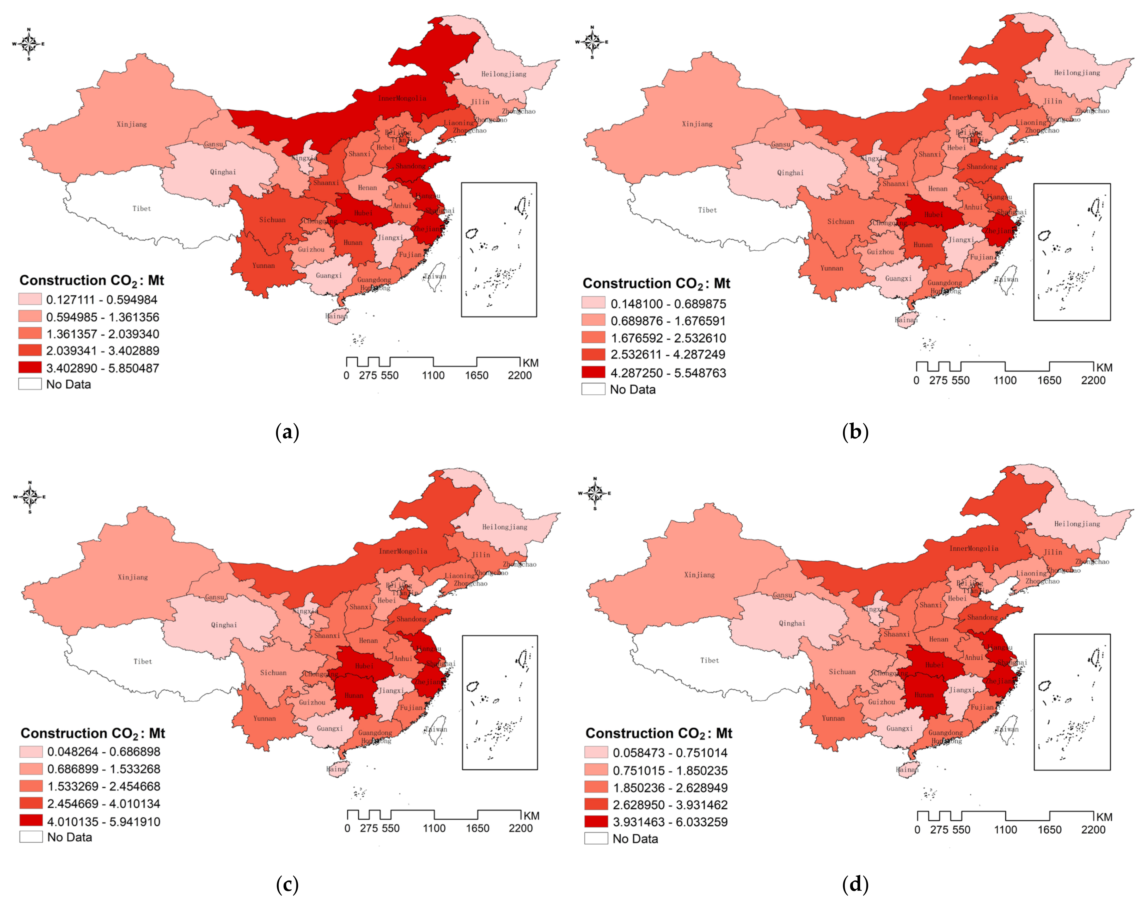
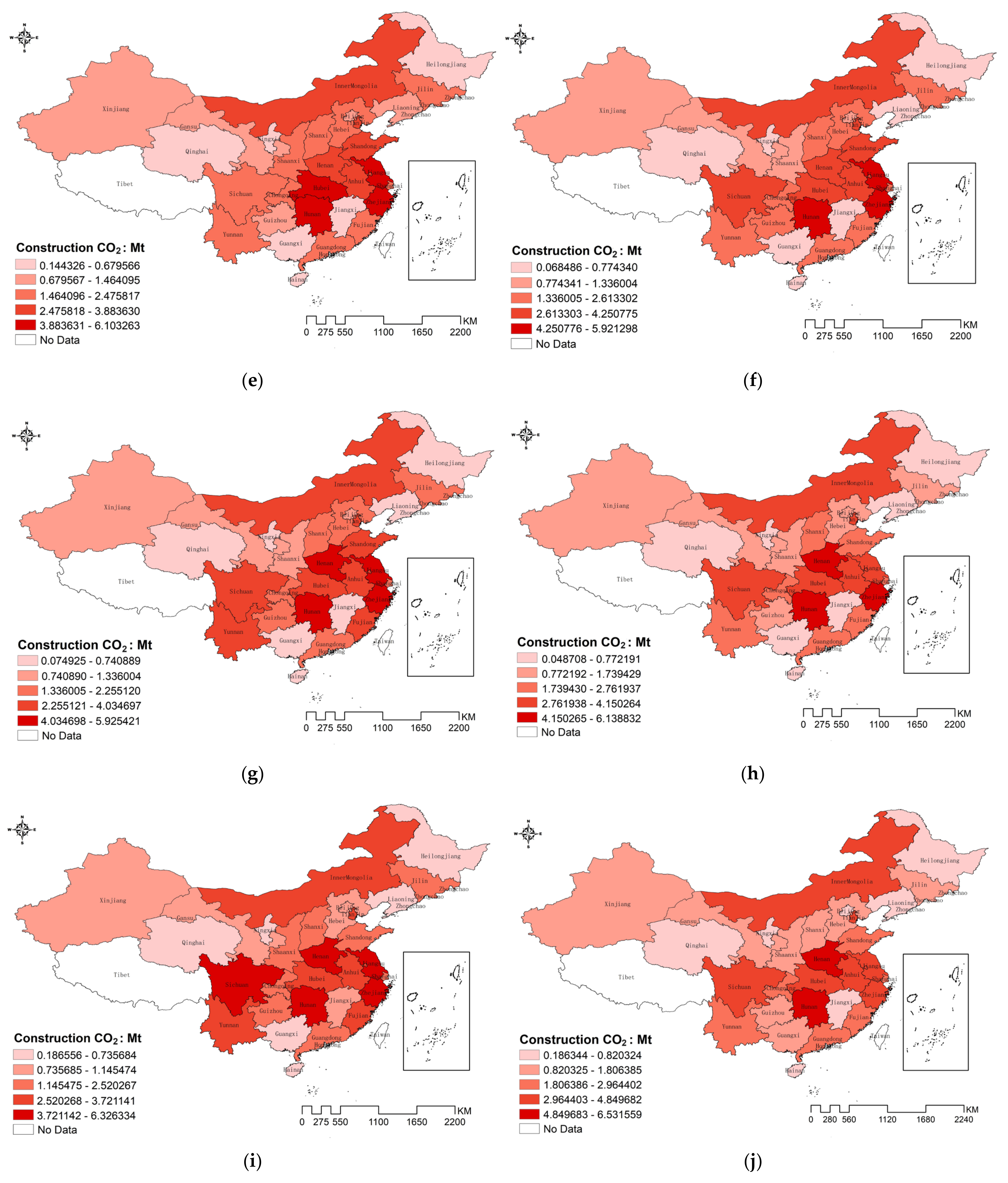
Figure 3.
Trend Analysis of carbon emissions in 2011 and 2020: (a) represents the year 2011; (b) represents the year 2020.
Figure 3.
Trend Analysis of carbon emissions in 2011 and 2020: (a) represents the year 2011; (b) represents the year 2020.

Table 1.
Variables and data definitions.
| Variables | Definition | Unit |
|---|---|---|
| CE | Carbon emissions in the construction industry | MT |
| GP | Gross product of the construction industry | 1010 Yuan |
| NE | Number of employees in the construction industry | 106 Person |
| UR | Urbanization rates | % |
| TR | Technological equipment rates | 104 Yuan/Person |
| PG | Domestic Patents Granted | 104 Item |
Table 2.
Descriptive statistics of carbon emissions in 30 provinces from 2011 to 2020.
| Year | 2011 | 2012 | 2013 | 2014 | 2015 | 2016 | 2017 | 2018 | 2019 | 2020 |
|---|---|---|---|---|---|---|---|---|---|---|
| Valid (n) | 30 | 30 | 30 | 30 | 30 | 30 | 30 | 30 | 30 | 30 |
| Null (n) | 0 | 0 | 0 | 0 | 0 | 0 | 0 | 0 | 0 | 0 |
| Mean | 2.080 | 2.044 | 2.170 | 2.204 | 2.261 | 2.242 | 2.305 | 2.263 | 2.308 | 2.334 |
| Median | 1.760 | 1.786 | 2.117 | 1.974 | 1.929 | 2.063 | 2.000 | 1.858 | 1.962 | 1.874 |
| Standard Deviation | 1.505 | 1.421 | 1.528 | 1.588 | 1.635 | 1.534 | 1.578 | 1.610 | 1.649 | 1.680 |
| Minimum | 0.127 | 0.148 | 0.048 | 0.058 | 0.144 | 0.068 | 0.075 | 0.049 | 0.187 | 0.186 |
| Maximum | 5.850 | 5.549 | 5.942 | 6.033 | 6.103 | 5.921 | 5.925 | 6.139 | 6.326 | 6.532 |
| 25% | 0.893 | 0.953 | 1.111 | 1.129 | 1.026 | 1.047 | 1.062 | 0.988 | 0.996 | 1.072 |
| 75% | 2.828 | 2.710 | 2.577 | 2.747 | 3.011 | 3.101 | 3.331 | 3.353 | 3.411 | 3.616 |
Table 3.
Moran’s I index from 2011 to 2020.
| Year | Moran’s I | p-Value | z-Value |
|---|---|---|---|
| 2011 | 0.151 | 0.015 | 2.1739 |
| 2012 | 0.142 | 0.011 | 2.1638 |
| 2013 | 0.162 | 0.004 | 2.4164 |
| 2014 | 0.194 | 0.001 | 2.8491 |
| 2015 | 0.225 | 0.001 | 3.2964 |
| 2016 | 0.245 | 0.001 | 3.3674 |
| 2017 | 0.279 | 0.001 | 3.8362 |
| 2018 | 0.284 | 0.001 | 3.8130 |
| 2019 | 0.281 | 0.001 | 3.8397 |
| 2020 | 0.269 | 0.001 | 3.5399 |
Table 4.
Comparison of model results.
| Index | Spatial Error Model | Spatial Lag Model |
|---|---|---|
| R2 | 0.700504 | 0.602019 |
| Sigma2 | 0.787003 | 1.0458 |
| S.E of regression | 0.887132 | 1.02264 |
| LogL | −41.209947 | −43.9397 |
| AIC | 94.4199 | 101.879 |
| SC | 102.827 | 111.688 |
Table 5.
Estimation results of Spatial Error Model.
| Year | 2011 | 2012 | 2013 | 2014 | 2015 | 2016 | 2017 | 2018 | 2019 | 2020 |
|---|---|---|---|---|---|---|---|---|---|---|
| GP | 0.0825 (1.68) * | 0.0464 (1.10) | 0.0438 (1.04) | 0.0414 (0.86) | 0.0319 (0.81) | 0.0481 (1.93) * | 0.0579 (2.36) ** | 0.0499 (2.24) ** | 0.0532 (3.08) *** | 0.0673 (3.65) *** |
| NE | 0.5959 (2.40) ** | 0.7659 (2.64) *** | 0.8008 (2.78) *** | 0.5143 (1.79) * | 0.7875 (3.22) *** | 0.6436 (4.45) *** | 0.4638 (3.30) *** | 0.3972 (2.26) ** | 0.2748 (1.58) | 0.2763 (1.55) |
| UR | 0.0065 (0.46) | 0.0083 (0.50) | 0.0333 (2.25) ** | −0.0063 (−2.89) | 0.0154 (0.68) | 0.0011 (0.06) | 0.0183 (1.07) | 0.0200 (0.99) | 0.0396 (2.14) ** | 0.0469 (1.97) ** |
| TR | 0.4492 (2.35) ** | 0.2619 (1.85) * | 0.0276 (0.33) | 0.5544 (2.10) ** | 1.0375 (2.15) ** | 0.6840 (2.62) *** | 0.4232 (1.52) | −0.2591 (−0.20) | −0.1624 (−1.68) * | −0.1170 (−1.98) ** |
| PG | −0.0618 (−0.94) | −0.1197 (−1.85) * | −0.1658 (−2.22) ** | −0.0242 (−0.30) | −0.1287 (−2.01) ** | −0.0717 (−1.73) * | −0.0710 (−2.05) ** | −0.0623 (−2.40) ** | −0.0760 (−3.38) *** | −0.0640 (−3.48) *** |
| LAMBDA | −0.4461 (−1.66) * | −0.5210 (−1.96) * | 0.6602 (−2.56) ** | −0.1840 (−0.53) | 0.4394 (1.61) | −0.8849 (−3.75) *** | −0.9191 (−3.97) *** | −0.9783 (−4.38) *** | 0.8722 (−3.67) *** | −0.9980 (−4.53) *** |
Note: The data in parentheses are the z-value. *, **, and *** represent the significant level of 10%, 5%, and 1%, respectively.
Disclaimer/Publisher’s Note: The statements, opinions and data contained in all publications are solely those of the individual author(s) and contributor(s) and not of MDPI and/or the editor(s). MDPI and/or the editor(s) disclaim responsibility for any injury to people or property resulting from any ideas, methods, instructions or products referred to in the content. |
© 2023 by the authors. Licensee MDPI, Basel, Switzerland. This article is an open access article distributed under the terms and conditions of the Creative Commons Attribution (CC BY) license (https://creativecommons.org/licenses/by/4.0/).
Share and Cite
MDPI and ACS Style
Yang, J.; Zheng, X. The Spatiotemporal Distribution Characteristics and Driving Factors of Carbon Emissions in the Chinese Construction Industry. Buildings 2023, 13, 2808. https://doi.org/10.3390/buildings13112808
AMA Style
Yang J, Zheng X. The Spatiotemporal Distribution Characteristics and Driving Factors of Carbon Emissions in the Chinese Construction Industry. Buildings. 2023; 13(11):2808. https://doi.org/10.3390/buildings13112808
Chicago/Turabian StyleYang, Jun, and Xiaodan Zheng. 2023. "The Spatiotemporal Distribution Characteristics and Driving Factors of Carbon Emissions in the Chinese Construction Industry" Buildings 13, no. 11: 2808. https://doi.org/10.3390/buildings13112808
Note that from the first issue of 2016, this journal uses article numbers instead of page numbers. See further details here.