The Numerical Simulation Study of Pumping Airflow Driven by Wind Pressure for Single- and Multi-Room Buildings

Abstract

Pumping airflow occurs in single-sided natural ventilation buildings when the openings are located on the leeward side; the direction of airflow through the building then changes periodicity. In order to propose a calculation method of the ventilation rates for single-room buildings and analyze the pumping ventilation for multi-room buildings, the CFD method with an SST k-ω turbulence model was used to conduct numerical simulation in this study, which is verified by other experimental results. Firstly, the qualitative and quantitative characteristics of pumping ventilation were investigated for a single-room building with two openings. The results show that the steady-state method underestimates the ventilation flow rates, and the unsteady-state method captures the microstructures of the flow better. Secondly, the vortex-shedding and indoor airflow oscillation frequencies were analyzed based on transient simulation for a single-room building. It was found that both of them increase with air speed. Then, the factors affecting ventilation flow rates were analyzed. A calculation method for dimensionless ventilation rates is proposed. Finally, the pumping ventilation for a multi-room building was numerically simulated. The ventilation rate for a middle room is greater than that for a corner room, and the ventilation rate for any room in a multi-room building is greater than the single-room building given the same room size and the same incoming wind speed. The findings of this paper are helpful for the design and evaluation of natural ventilation.

1. Introduction

Natural ventilation is an important passive technology for buildings, because its appropriate application can conserve energy and supply fresh outdoor air. Natural ventilation can be divided into single-sided ventilation and cross-ventilation. Many studies have shown that cross-ventilation is superior to single-side ventilation in the field of indoor ventilation [1,2], but in most cases, single-side ventilation is still very important in building design, as few buildings can be cross-ventilated due to internal zoning, fire codes, safety requirements and privacy issues.

Single-side ventilation systems can be categorized by their number of openings: a single opening (SS1) and multiple openings (SSn). In the former, air must enter and exit through the same openings, while in the latter, there is a clearer division of air entering and exiting the room [3]. It has been found that multiple openings provide a better ventilation effect than a single opening [4]. The unilateral natural ventilation model proposed by Warren [5] is suitable for the estimation of ventilation rates in most cases. In single-side ventilation, unsteady natural ventilation mechanisms are classified into continuous airflow, pulsating flow, eddy penetration and diffusion phenomena [6].

The ventilation is induced by the vortex shedding of the airflow around the building, which is referred to as the pumping airflow [7]. It can be considered as a special type of eddy penetration. In 2016, Daish et al. [7] first analyzed the pumping airflow of the SS2 model, which has two openings located on the leeward side of the structure. The ventilation airflow in this instance oscillated with the Strohal frequency for time T, exhibiting a unique periodic fluctuation in flow.

In 2018, the pumping airflow was also observed by Zhong [8] in a 2D CFD simulation, and the impact of the building aspect ratio, incoming wind speed, and opening spacing on the frequency and ventilation flow rate of the pumping flow was examined. The two-dimensional simulation method, however, was unable to accurately capture three-dimensional flow properties. In 2019, Zhong carried out quasi-3D numerical simulation, and they found that the increasing trend in the dimensionless ventilation flow rate disappears or even decreases as the wind speed increases to 5 m/s. The dimensionless ventilation flow rate increased as the aperture separation increased, but it had no effect on the vortex-shedding frequency [9]. In 2020, Daniel [10] pointed out that the studies proposed by Zhong et al. [8,9,11,12] did not consider the three-dimensional structure of the pumped ventilation flow in buildings. In 2021, Zhong [13] pointed out that the ventilation flow rate of the bottom and top floors of buildings is considerably different from that of the middle floors, because the ground and top floors of a building have a greater influence on vortex shedding. In 2021, Graça [14] found that there are particular wind angles that also cause pumping airflow, in addition to when the wind is perpendicular to the facade (single-sided rooms) or aligned with the building corner (corner rooms), when there were two openings in the same facade of a building.

In summary, pumping ventilation occurs when the two openings are located on the leeward side for single-room model buildings. The frequency change in the flow’s direction is related to the shedding frequency of the vortex street. Moreover, it was found that the pumping ventilation volume was related to the aperture separation: for example, Daish [7] stated that the ventilation flow rate increased with $s^{\prime 1/2}$ ($s^{\prime }$ is the aperture separation), while Kobayashi [15] and Daniel [10] concluded that the ventilation flow rate was linearly related to $s^{\prime }$.

There are different conclusions about the relationship. In addition, previous research did not consider a multi-room building, which is the more realistic case. Does pumping ventilation still exist, and what is the difference for rooms in different locations? Aiming to answer these questions and further understand pumping ventilation, this paper analyzed the qualitative and quantitative characteristics of the pumping airflow of a single-room building, and it also investigated the pumping airflow of a multi-room building. Figure 1 shows the flow chart of this paper.

Revealing the principles of the natural ventilation is a prerequisite for further designing the thermal environment and evaluating the diffusion of pollutants. This study can provide references for understanding the mechanisms and effects of the natural ventilation.

2. Numerical Simulation Method

2.1. Model Simplification and Simulation Settings

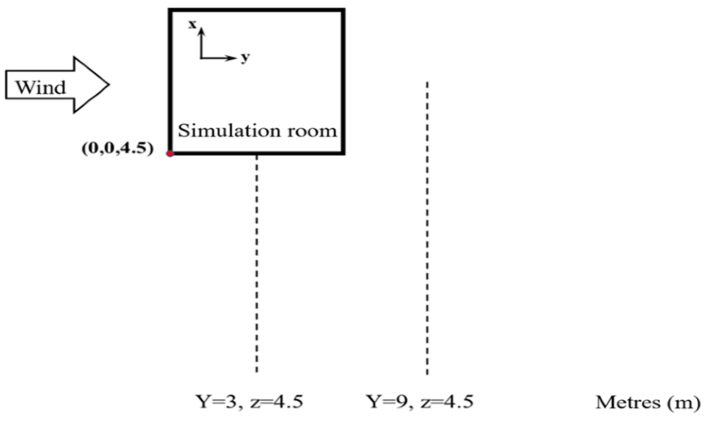
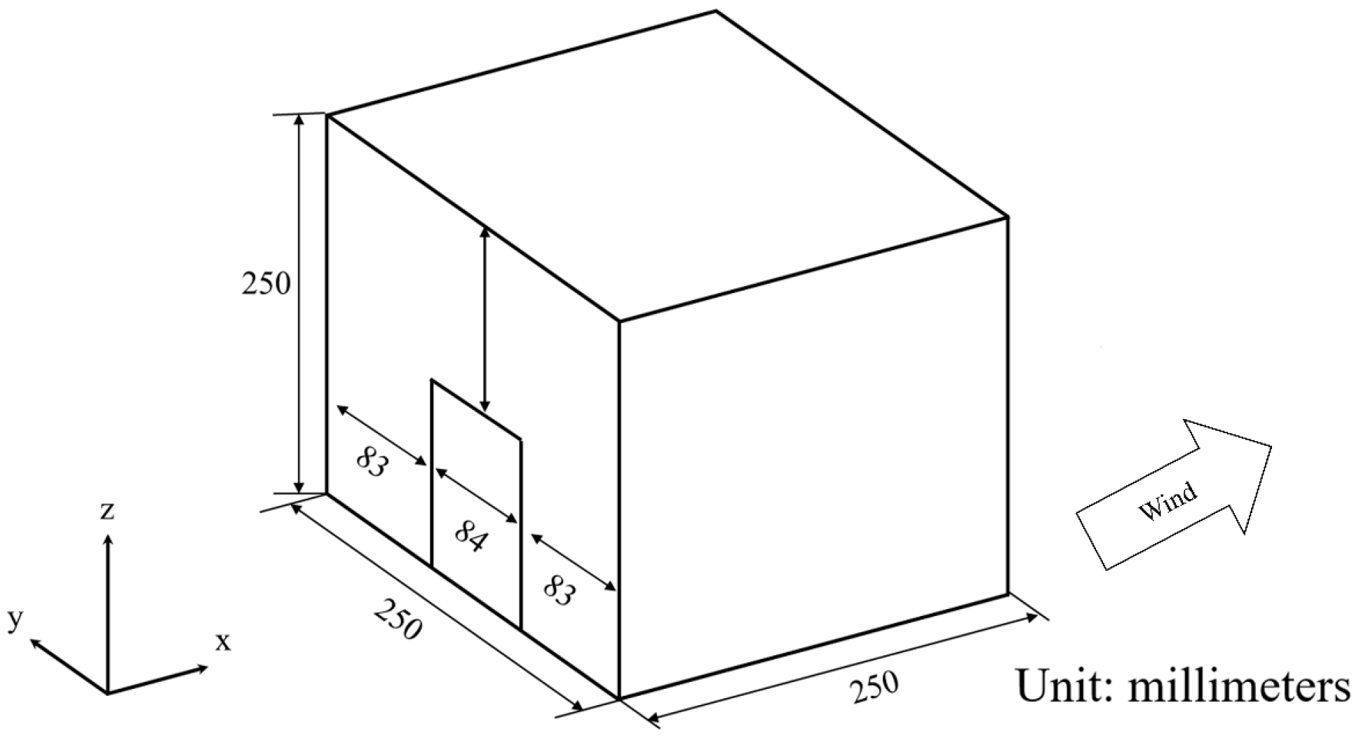
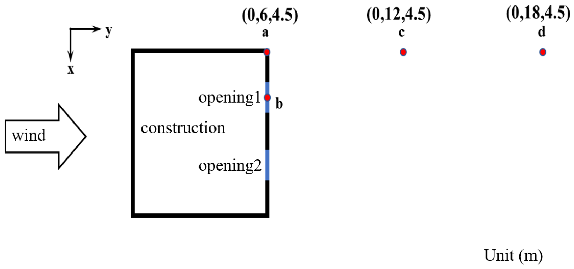
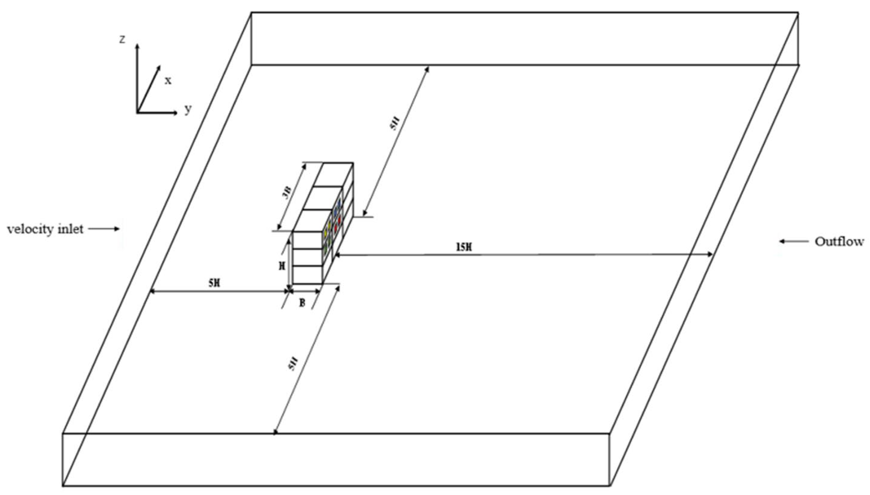
2.1.1. Computational Geometry and Domain

A three-story building was taken as the model 1 (e.g., Figure 2). The total height of the building H is 9 m, and there is one room on each floor. The dimension of each room is 6 m × 6 m × 3 m (B × B × 1/3 H). The natural ventilation room is located on the second floor with two leeward openings of the same size: 1 m × 1 m. The centers of the two openings are 3 m apart and 1.5 m from the respective closer sides of the building. The three rooms in the building are not connected to each other and are separated by floors or ceilings.

The computational domain has a significant impact on the simulation results, and the blocking ratio is thought to be important [16], which meant that it should be less than 3% of the computational domain size. Additionally, for the building body, the computational domain’s sides, the top, and the external exit boundary all need to be at least 5 H and 10 H away from the building, respectively. The computational domain is 186 m × 96 m × 9 m in size because only the quasi-3D building case was taken into account in this study, which meant that the height of the computational domain was equal to the height of the building, the side distance is 5 H, and the distance from the leeward side to the exit is 15 H. The blockage ratios of it are less than 3%. Due to the fact that the pumping flow involved two apertures and that the spacing between the two openings has an impact on the airflow, three cases with varying spacing are adopted in this paper (e.g., Figure 3). The quoted dimensionless aperture distance is

$$s^{\prime }=\frac{s}{B}$$

(1)

where s is the distance (in meters) between the centers of the two openings, and B is the building’s width (in meters), using 0.25, 0.5, and 0.75 as examples.

2.1.2. Numerical Simulation Settings

Solution Settings

In this paper, the finite volume method was used to solve the governing equation. The governing equation was as follows:

$$\frac{\partial \rho }{\partial t}+\frac{\partial \left(\rho u\right)}{\partial x}+\frac{\partial \left(\rho v\right)}{\partial y}+\frac{\partial \left(\rho w\right)}{\partial z}=0$$

(2)

$$\rho \frac{\partial \overrightarrow{u}}{\partial t}+\rho \overrightarrow{u}·\overrightarrow{\nabla }·\overrightarrow{u}=-\overrightarrow{\nabla }p+\overrightarrow{\nabla }·\tau +\left(\rho -{\rho }_{\infty }\right)g$$

(3)

$$\frac{\partial T}{\partial t}+u\frac{\partial T}{\partial x}+v\frac{\partial T}{\partial y}+w\frac{\partial T}{\partial z}=\frac{\lambda }{\rho c_p}\left(\frac{{\partial }^{2}T}{\partial x^2}+\frac{{\partial }^{2}T}{\partial y^2}+\frac{{\partial }^{2}T}{\partial z^2}\right)+\frac{S_T}{\rho }$$

(4)

The three-dimensional RANS equations were solved together with the k-ω shear stress transport (SST k-ω) model:

$$\frac{\partial \rho k}{\partial t}+\frac{\partial \left(\rho u_{i}k\right)}{\partial x_i}={{\tau }_i}_j\frac{\partial u_i}{\partial x_j}-{\beta }^{*}\rho \omega k+\frac{\partial }{\partial x_j}\left[\left(\mu +{\sigma }_k{\mu }_t\right)\frac{\partial k}{\partial x_j}\right]$$

(5)

$$\frac{\partial \rho \omega }{\partial t}+\frac{\partial \left(\rho u_i\omega \right)}{\partial x_i}=\frac{\gamma }{{\nu }_t}{\tau }_{ij}\frac{\partial u_i}{\partial x_j}-\beta \rho {\omega }^2+\frac{\partial }{\partial x_j}\left[\left(\mu +{\sigma }_{\omega }{\mu }_t\right)\frac{\partial \omega }{\partial x_j}\right]+2\left(1-F_1\right)\rho {\sigma }_{\omega 2}\frac{1}{\omega }\frac{\partial k}{\partial x_j}\frac{\partial \omega }{\partial x_j}$$

(6)

This paper assumed that the external wind speed was stable and the supply air parameters were constant. In addition, the air in the fluid region was considered to be an incompressible ideal gas. The SIMPLE method was chosen to the pressure–velocity coupling, and the PRESTO! pressure interpolation format was chosen. The controlling equations were discretized as the second-order windward terms because second-order discretization has a higher precision than the first-order discretization. With the exception of the energy equation residuals, which were 1 × 10⁻⁶, the convergence criterion for the system of equations was 1 × 10⁻⁹ for all parameter residuals. The steady-state simulation was carried out firstly, and then the results were adopted as the initial conditions in the transient calculation.

For transient calculations, a time step which is too large or too small will affect the results. The CFL number can be used to determine the appropriate time step.

$$\Delta t=CFL\times \frac{l}{U}$$

(7)

where l is the distance from wall to the first grid, and the value of that is 0.01 m in this study. The CFL value for the explicit solver is close to 1, and for the implicit solver, it will be increased to a higher number [17]. The research [18] showed that the smaller time-step difference had a limited impact on the outcomes when the time-step length was substantially less than the vortex-shedding duration; hence, CFL may be considered as 10 [9]. When the incoming wind speed is 1 m/s, $∆t$ is calculated as 0.1 s.

Table 1. Time steps at different wind speeds.

U (m/s)	$\mathit{R}\mathit{e}$	$∆\mathit{t}$ (s)
1	410,752	0.100
2	821,504	0.050
3	1,232,256	0.033
4	1,643,008	0.025
5	2,053,761	0.020

displays the time step changing with wind speed. A total of 10~20 iterations were run in each time step to ensure accurate calculation results.

Boundary Conditions

The velocity inlet boundary condition was adopted to the inlet, with U_y values of 1 m/s, 2 m/s, 3 m/s, 4 m/s, 5 m/s, and the velocity in the other two directions was 0; the turbulence intensity at the inlet was set to 10%, and the turbulence integration length was set to 0.58 m [19]. The outlet was set as outflow; the sides, the top and the bottom were set as symmetry; the opening was set as the interior, and all the other wall surfaces were set as no-slip.

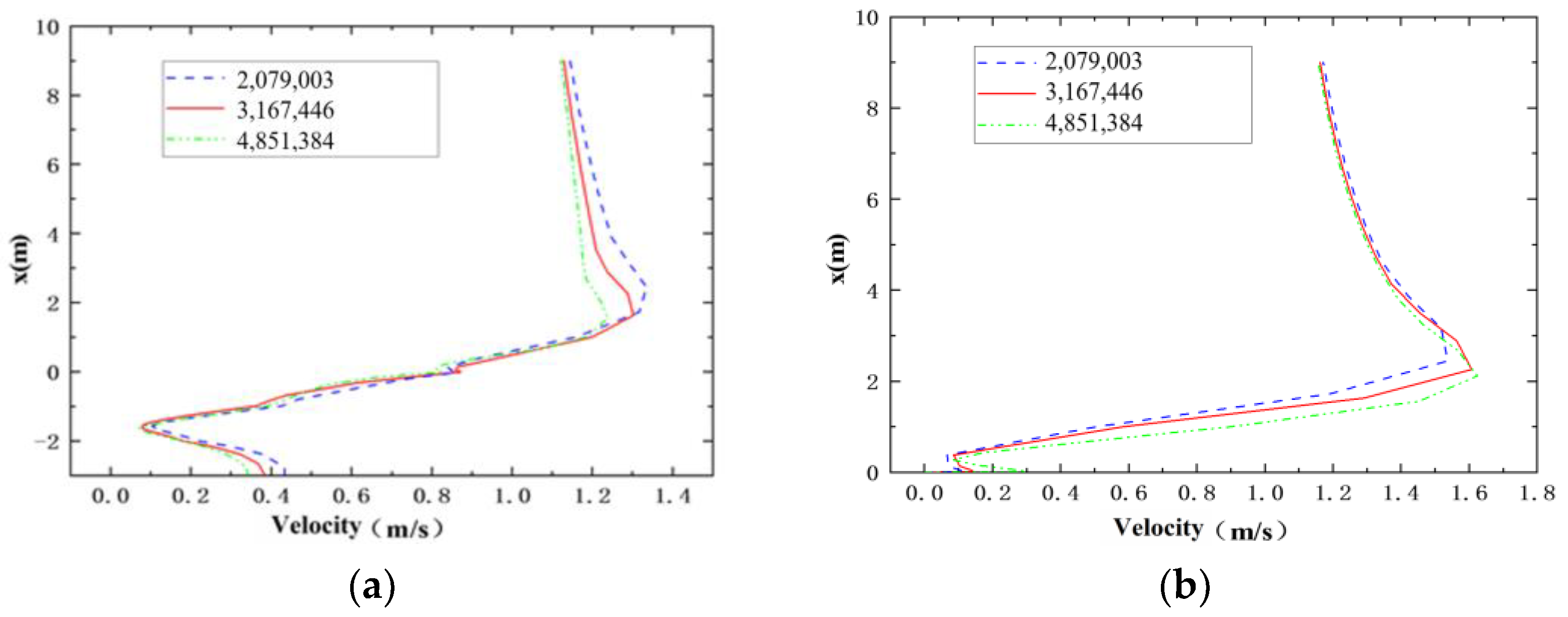
Grid Division and Independence Verification

The domain was constructed using the hexahedral gird (Figure 4). The grid was refined in the opening and the near-wall. For the case of s′ = 0.5, three grid schemes with the grid numbers of 2,079,003, 3,167,446, and 4,851,384 were selected for independence verification. The corresponding y+ values for the three-grid method were 45, 30 and 15, and the minimum distances of the grids from the wall were 0.015 m, 0.01 m, and 0.005 m, respectively. The monitoring line Y = 3 m, and Y = 9 m in the plane with a Z value of 4.5 m is chosen for the sample set (Figure 5). The results with different numbers of grids are shown in Figure 6. As can be seen, the changing rules of the wind speed outside the building showed the same trend. Based on the results, the grid number of 3,167,446 (Figure 4) is finally selected for the case, as a further increase in the mesh density does not produce obvious changes in the numerical solutions.

2.1.3. Validation of CFD Methodology

In 2003, Jiang et al. [20] conducted a wind tunnel experiment for natural ventilation. The study focused on a small (0.25 cubic) building model with a window opening size 0.084 m × 0.125 m (length × height), as shown in Figure 7. There is a workspace with the area of 2.0 m × 2.0 m, and the height 1.0 m, which is in the wind tunnel. The velocity measurements were conducted on a grid plane at the center of the building. In order to verify the CFD method used in this paper, Jiang’s case was chosen for the numerical simulation. The downstream length was set as 8 H; the upstream length was 4 H; and the lateral length was 4 H on both sides of the building in the computational zone. The total number of the grids was 969,570. The boundary conditions and the wind speed were consistent with the literature, and the turbulence model was the SST k-ω. The numerical results are shown to have good agreement with the experimental data, and the relative error is less than 20% in the most regions (Figure 8). Therefore, the CFD method adopted in the paper was validated for the numerical simulation of the natural ventilation.

2.2. Comparison of Steady-State and Transient Simulation

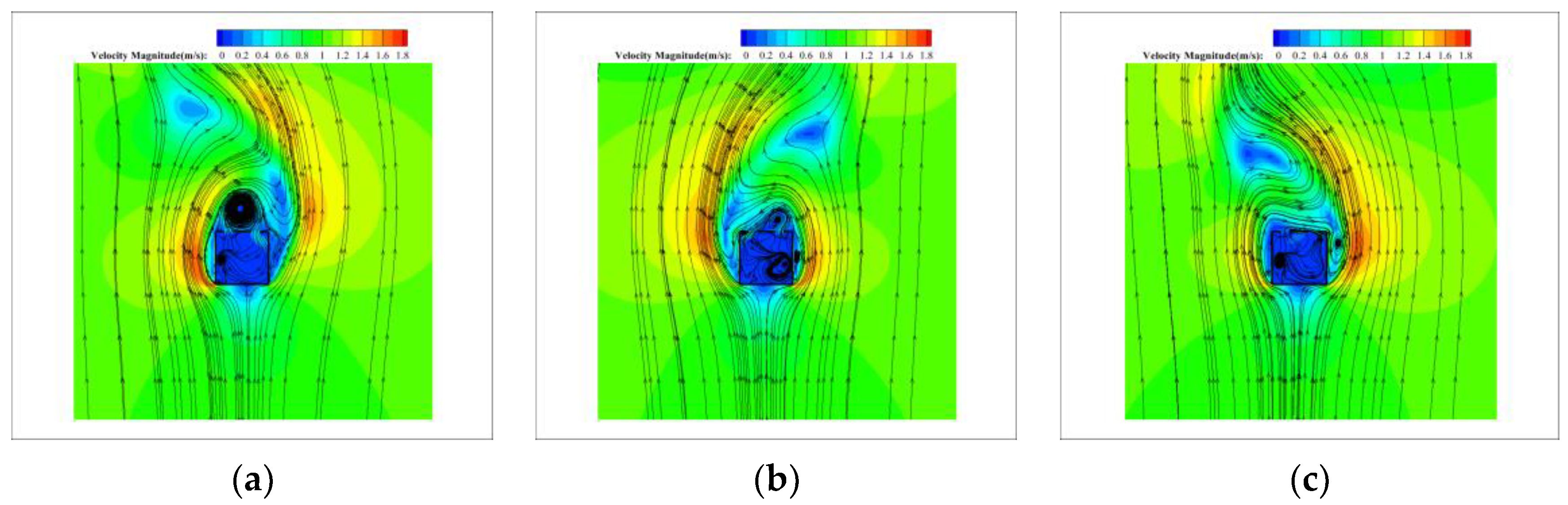
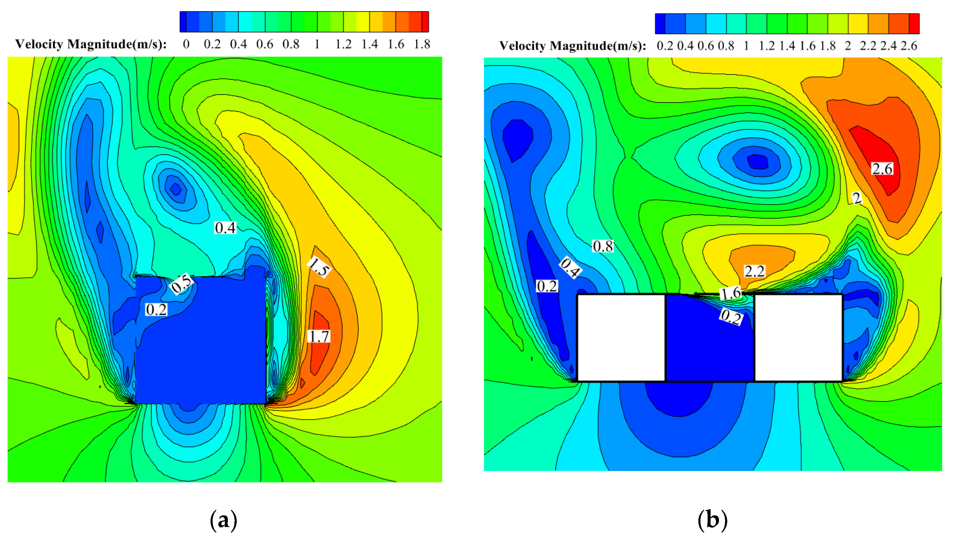
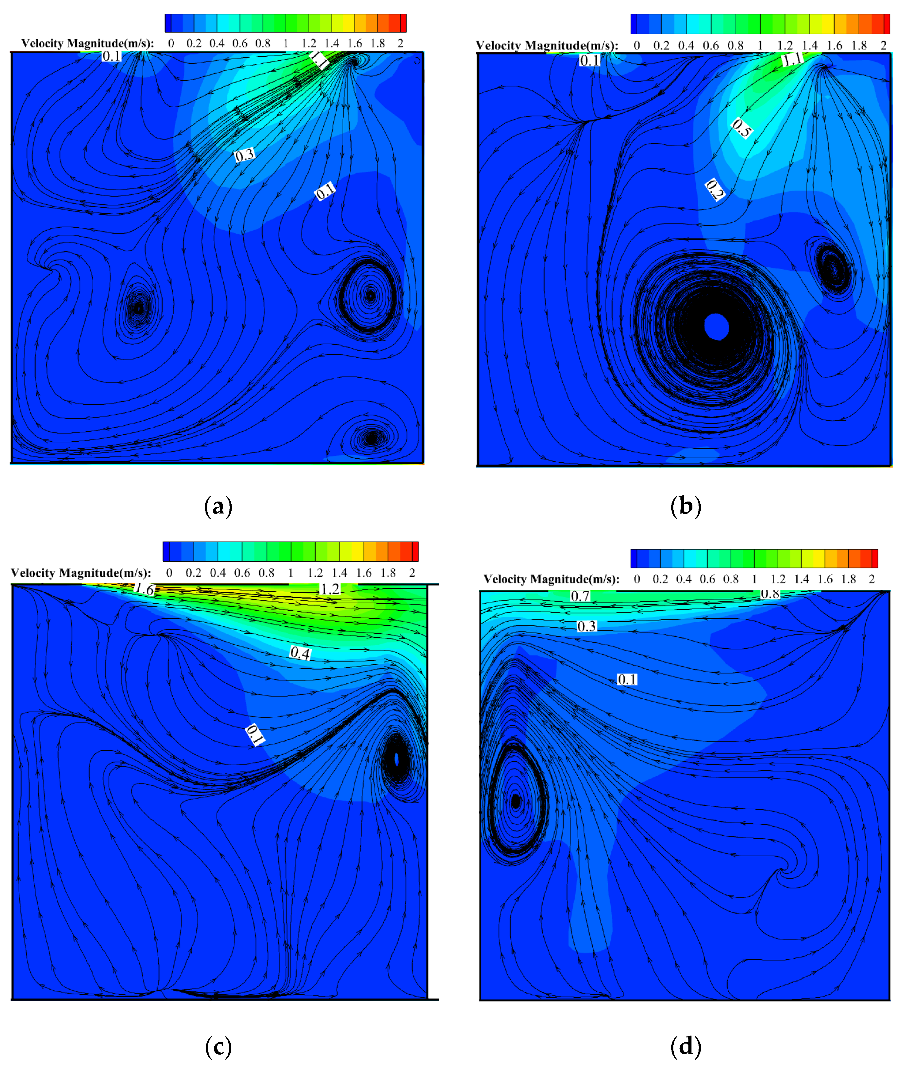
2.2.1. The Flow Field

The transient simulation can describe the small structures in turbulent better than steady-state calculation. For example, as shown in Figure 9 (incoming wind speed was 1 m/s), there was an obvious vortex street in the building wake in the transient simulation compared to the steady-state results.

Figure 10 depicts the y-direction velocity cloud charts at the openings on the leeward side of the room, where the steady-state result did not have a symmetric image and the velocity distribution was rather uniform. The unsteady-state calculation revealed that the velocity distribution was symmetric about z = 4.5 m, where the minimum velocity was located at one of the openings and the maximum velocity was located near the wall. In general, there is a significant difference in the calculation results between the transient calculation and the steady-state calculation because the latter result is the average value.

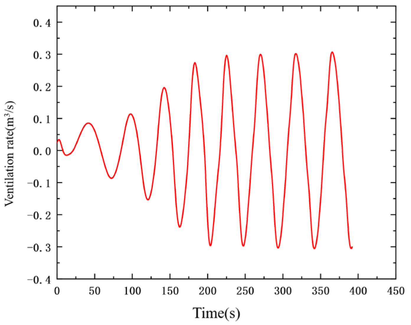
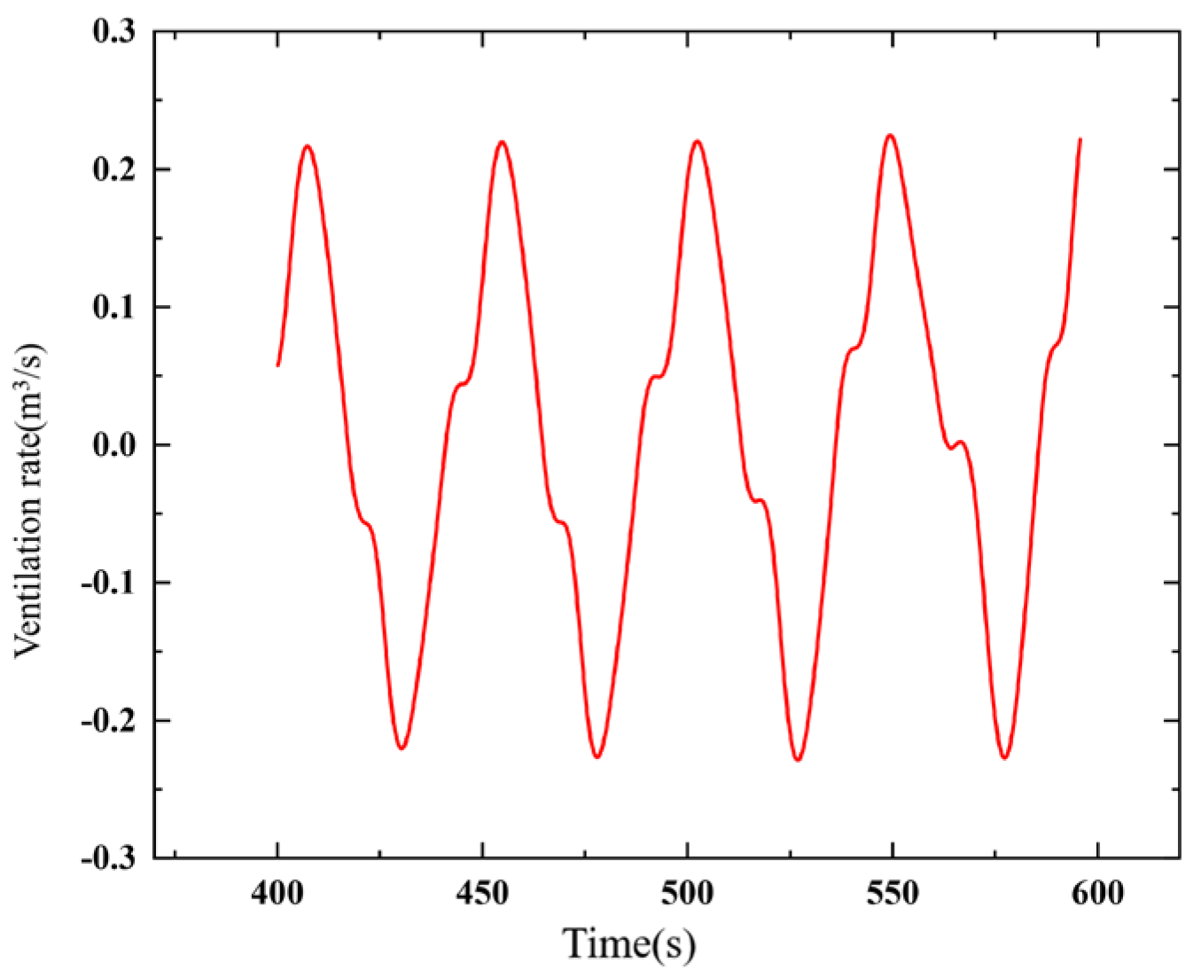
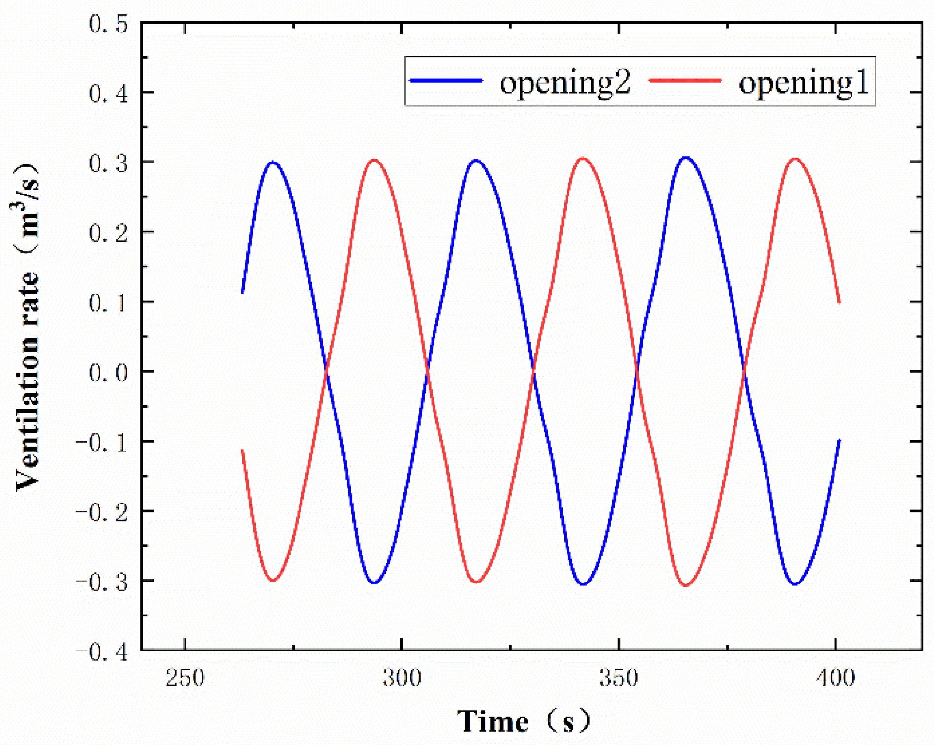
2.2.2. The Ventilation Flow Rates

The ventilation flow rates are also compared here (

Table 2. Results for different cases.

Wind Speed (m/s)	Q_(Steady State) (m3/s)	Q_(Unsteady State) (m3/s)
1	0.0778	0.1356
2	0.3018	0.3389
3	0.4207	0.5120

). The steady-state case results could be obtained directly; however, the ventilation flow rate is the average of the total ventilation volume for each time step with the entire period in the non-stationary calculation.

It can be seen that the steady-state calculation underestimates the ventilation flow rates of the building. The transient simulation method is more accurate because it takes into account the fluctuation of the wind around the buildings. Therefore, the method of the unsteady-state simulation was selected in the following calculation.

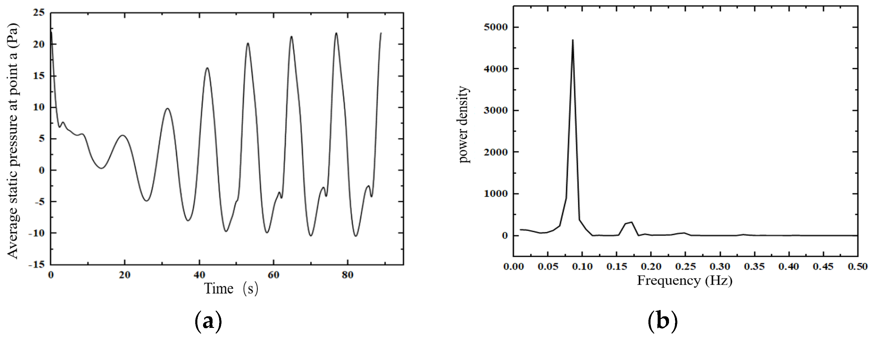
2.2.3. Periodic Characteristics of Pumping Airflow

The detailed flow field and the periodic characteristics of the typical pumping airflow are analyzed in this section. The case is the same as that in Section 2.2.1. Figure 11 displays the streamline distribution of the flow field with the cross-section situated at Z = 4.5 m.

The flow around buildings in a natural wind field is similar to the flow around a blunt body. As shown in Figure 11, the incoming air flow separated on the building’s windward surface and flowed to its two sides. As a result of the pressure difference, a clockwise vortex formed on the left side of the surface. Next, a separation was created at the backward corner of the left surface, and the vortex gradually grew to the entire leeward surface.

The airflow at the back of the building was forced to enter the building through the opening on the right side, create a circulating airflow that followed the vortex’s direction, and exit through the opening on the left. The airflow on the opposite side, however, was exactly the opposite. It formed an anti-clockwise vortex on the right side surface. This caused the airflow to enter the room through the left side opening after separating and attaching itself to the leeward surface at the rear corner point of the lower right side. It then formed a circulating airflow that flowed out of the right side opening in the same direction as the vortex in an anti-clockwise direction.

Vortices were produced and shed alternatively on the either side of the square building, finally forming a regular vortex street in the wake flow. As a result, the fluctuating ventilation named as the pumping airflow was generated. Figure 12 describes the ventilation flow rates of the building changing with time. During the first 200 s, the changing amplitude of the ventilation flow rates was increasing gradually because the vortex shedding of the airflow was still in the developmental stage. After that, the change in amplitude decreased to form the regular fluctuations similar to the sinusoidal form. From Figure 13, it can be discovered that not all of the ventilation flow rates change with the sine wave, especially when the opening spacing was adjusted. However, all the cases clearly displayed the features of a regular fluctuation.

3. Result and Discussion

3.1. Pumping Airflow in a Single-Room Building

In this part, the numerical simulation was used to examine the features of the pumping airflow with different incoming wind speed in a single-room building. The vortex-shedding frequency and the ventilation flow rates were analyzed.

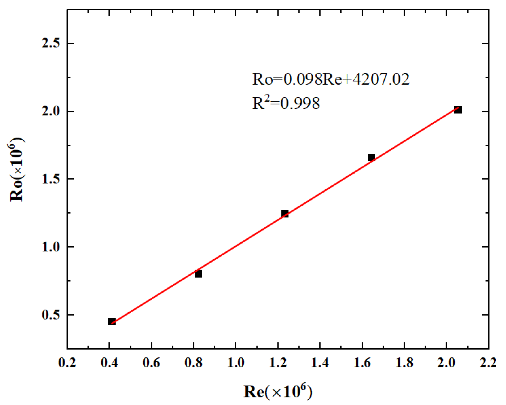
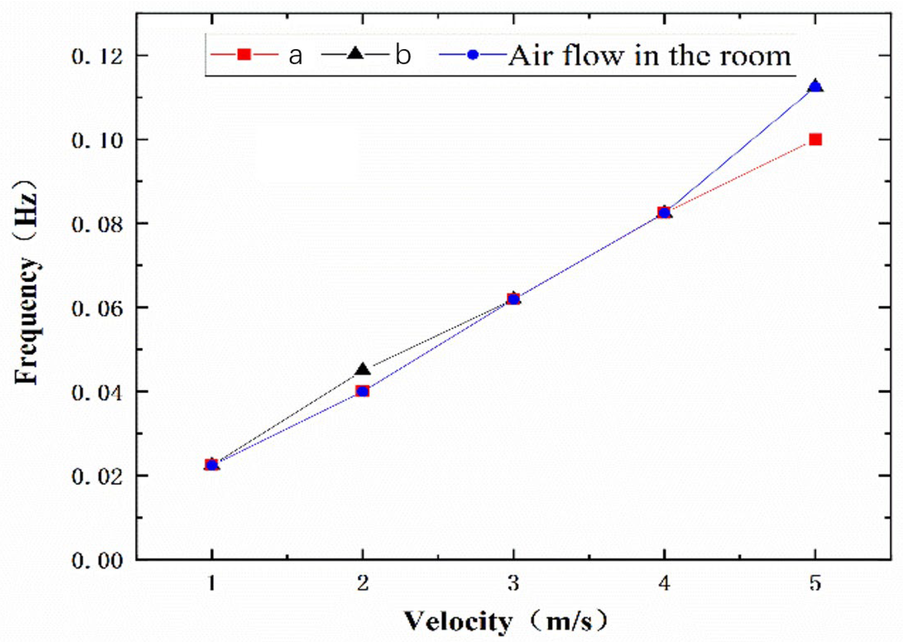
3.1.1. Fluctuating Frequency

Vortex-Shedding Frequency

Four monitoring points were selected in order to analyze the vortex-shedding frequency, as shown in Figure 14. Point b was located at the center of the opening 1 with a height of 4.5 m. The time-domain and the frequency spectrum plots of the static pressure at point a with the incoming wind speed as 4 m/s are presented in Figure 15a,b, respectively. As shown in the time-domain plot, the static pressure changed periodically. From the frequency spectrum plot, it was possible to determine that the shedding frequency was 0.0825 Hz, at which the power spectral density achieves its maximum value.

The vortex-shedding frequencies of the four points with different wind speed are presented in

Table 3. Frequency of vortex shedding at 4 points under different wind speeds.

Position Frequency (Hz) Velocity (m/s)	a	b	c	d
1	0.0224	0.0224	0.0224	0.0224
2	0.0400	0.0400	0.0400	0.0400
3	0.0619	0.0619	0.0619	0.0619
4	0.0825	0.0825	0.0825	0.0825
5	0.1000	0.1125	0.1000	0.1000

. It was evident from the simulated data that with the same wind speed, the vortex-shedding frequencies essentially stayed constant at different places. The frequency at point b increased by 12.5% more than the other three places only at the case wind speed of 5 m/s. For various wind speeds, the frequency of vortex shedding at the same place increased as the wind speed rose.

As a dimensionless number used to describe fluid flow, the Reynolds number (Re) represents the ratio of inertial forces to viscous or frictional forces acting on a moving object. In the research of the wind field around buildings, the dimensionless number Strauhl number (St) was also utilized to investigate the flow frequencies.

$$Re=\rho dU/\mu$$

(8)

$$St=df/U$$

(9)

where d was the characteristic length of the object (m); μ was the dynamic viscosity (N·m/s²); U was the velocity (m/s); and f was the frequency (Hz).

Due to the fact that the relationship between the Reynolds number and Strauhl number in the vortex-shedding frequency research was not linear, Roshko proposed another dimensionless number, Roshko number (Ro) [21]:

$$Ro=\frac{f{d}^2}{\nu }$$

(10)

where ν was the kinematic viscosity (${\mathrm{m}}^2/\mathrm{s}$). Previous studies had given the formulae for the corresponding $Ro$ numbers as follows [10,22]:

$$150<Re<250\hspace{1em}\hspace{1em}Ro=0.212Re-4.7$$

(11)

$$10^4<Re<4\times 10^4\hspace{1em}\hspace{1em}Ro=0.1477Re-138$$

(12)

where Equation (11) was obtained in the flow field across a cylinder with a low Re number, while Equation (12) was obtained for the 3D square cylinder model.

Based on the numerical simulation results and combined with the Fourier transform, f and St were obtained. Using Equations (8) and (10), the Ro number and Re number were determined, and the results are provided in

Table 4. Parameter values with different wind speeds.

Parametric Velocity (m/s)	$\mathit{f}$ (Hz)	$\mathit{S}\mathit{t}$	$\mathit{R}\mathit{e}$	$\mathit{R}\mathit{o}$
1	0.0224	0.1346	410,752	55,205
2	0.0400	0.1200	821,504	97,758
3	0.0619	0.1237	1,232,256	152,553
4	0.0825	0.1237	1,643,008	203,240
5	0.1000	0.1200	2,053,761	246,451

. Daniel [10] discovered that the St values measured during vortex shedding in the 2D model case ranged from 0.07 to 0.21. In this study, the values of St in the quasi-3D model fell within the range of 0.12 to 0.14 and in a bandwidth of roughly 0.015. The result is relatively reasonable compared to the research of Daniel [10]. The following equation was developed by fitting the Re and Ro data using the least squares method, as shown in Figure 16.

$$4\times 10^5<Re<2.1\times 10^6\hspace{1em}\hspace{1em}Ro=0.098Re+4207.2$$

(13)

Therefore, it could be judged that there was also a good linear relationship between the Ro number and Re number in this study case, which was similar to that in other research.

Indoor Airflow Oscillation Frequency

During the simulations, the instantaneous ventilation flow rates of two openings were monitored. The results with wind speed as 1 m/s are shown in Figure 17, that positive ventilation values indicated the air flow into the room and negative values showed the air flow out. It could be seen that the ventilation flow rates of two openings were the same but the flow direction was opposite, and all of their sinusoidal properties changed with time.

Figure 18 depicts the oscillation frequency of the airflow with various wind speeds, showing there was a significant association between the oscillation frequency of the airflow and the wind speed. As the wind speed increased, the frequency of the oscillations inside the building rose. The airflow oscillation frequency was basically the same as the vortex-shedding frequency around the building; all of them varied monotonically with the wind speed, as shown in Table 3 and Figure 18. Moreover, if the dimensionless opening distances s′ changed from 0.25 to 0.5, the simulation results showed that the frequency was only different by about 5%. It could be concluded that the opening distance had almost no impact on the oscillation frequency of the indoor airflow.

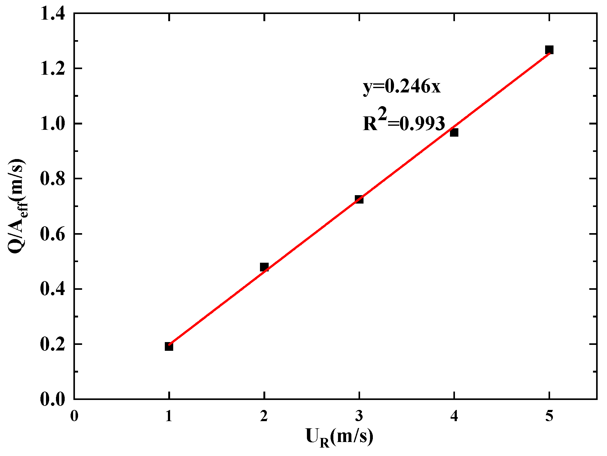
3.1.2. Ventilation Flow Rates

In the analysis of natural ventilation, the most important parameter is the ventilation flow rates. In this study, the dimensionless ventilation flow rates could be obtained by the following equation.

$$Q\prime =\frac{Q}{U_R{A}_{ref}}$$

(14)

where U_R is the reference wind speed (m/s), which is considered equal to the incoming wind speed in this study; A_ref is the reference opening area (m²).

The reference opening area is the effective opening area, which can be calculated by the formula:

$$A_{ref}=A_{eff}=\frac{A_1{A}_2}{{\left({A_1}^2+{A_2}^2\right)}^{1/2}}$$

(15)

where A₁ and A₂ are the areas (m²) of the two openings. In this study, A₁ = A₂ = A, so $A_{eff}=A/\sqrt{2}$.

According to the literature [23], the mean and fluctuating ventilation made up the instantaneous ventilation. The fluctuating ventilation rates can be predicted by the standard deviation as follows:

$${\sigma }_Q={\left[\frac{1}{N_m}{\sum }_1^{N_m}{\left(Q-Q_m\right)}^2\right]}^{1/2}$$

(16)

where σ_Q is the fluctuating ventilation (m³/s), N_m is the time step, Q is the monitored ventilation (m³/s), and $Q_m$ is the mean ventilation (m³/s), which is the average of the sequence of instantaneous ventilation changes over time. In addition, $\overline{Q}\prime$ and σ_Q′ represent the dimensionless numbers of the mean and fluctuating ventilation, respectively.

The Influence of Different Wind Speeds

The ventilation flow rates with different wind speeds are shown in

Table 5. Dimensionless mean and fluctuating ventilation flow rates with different wind speeds.

Velocity (m/s)	1	2	3	4	5
${\overline{Q}}^{\prime }$	0.1917	0.2397	0.2414	0.2420	0.2534
${{\sigma }_Q}^{\prime }$	0.1350	0.1320	0.1333	0.1335	0.1345
$Q$ (m3/s)	0.1356	0.3389	0.5120	0.6840	0.8960

. From the results, it can be seen that the dimensionless mean ventilation $\overline{Q}\prime$ is larger than the dimensionless fluctuating ventilation σ_Q′ for all the five cases. It may indicate that although there are periodic changes in the direction of ventilation airflow, the average ventilation intensity is greater than the fluctuating ventilation in terms of the overall pumping ventilation effect on the room. Moreover, the simulated results show that almost all the ventilation flow rates increased with the wind speed except the dimensionless fluctuating air volume under the condition of wind speed as 1 m/s. The probable reason is that there was more airflow (which on the vortex scale was smaller than the opening size) entering or exiting the room from the openings at lower wind speeds, which increased the dimensionless fluctuating air volume.

Based on the ventilation flow rates, incoming wind speed, and the effective opening area, the following formula can be obtained:

$$Q\prime =\frac{Q}{U_R{A_e}_{ff}}=0.246$$

(17)

The plot of the relationship after the data fitting and the Pearson’s correlation coefficient are shown in Figure 19, and its Pearson’s correlation coefficient (R²) is 0.993. It indicates that there is a strong linear correlation between the ventilation flow rates and the wind speeds.

Warren [5] previously proposed a unilateral natural ventilation model, which was considered the most accurate model suitable for single-sided ventilation [5,24]. In addition, Daish [7] carried out special research about the pumping ventilation. Therefore, the two models were applied here to compare the simulated results. Using the simulation results as the base value, the relative error was calculated as:

$$\epsilon =\frac{\left|Q_m-Q_n\right|}{Q_n}\times 100\%$$

(18)

where ε is the relative error (%); Q_m is the ventilation flow rates volume obtained by existing model (m³/s); and Q_n is the numerically simulated ventilation flow rate (m³/s).

The comparison results are shown in

Table 6. Ventilation flow rates obtained from different calculation models.

Wind Speed (m/s)	${\mathit{Q}}_{\mathit{n}}$ (m3/s)	Daish ${\mathit{Q}}_{\mathit{D}\mathit{a}\mathit{i}\mathit{s}\mathit{h}}$ (m3/s)	Daish $\mathit{\epsilon }$ (%)	Warren ${\mathit{Q}}_{\mathit{W}\mathit{a}\mathit{r}\mathit{r}\mathit{e}\mathit{n}}$ (m3/s)	Warren $\mathit{\epsilon }$ (%)
1	0.1356	0.1928	42.19	0.0500	63.13
2	0.3389	0.3856	13.79	0.1000	70.49
3	0.5120	0.5784	12.98	0.1500	70.70
4	0.6840	0.7712	12.76	0.2000	70.76
5	0.8960	0.9640	7.600	0.2500	72.10

. The model of the Warren underestimated the ventilation flow rates to a greater extent with the average error about 70%. The results of Q_Daish were closer to the numerical data than the Warren model, with the relative error smaller than 15%, except for the wind speed of 1 m/s. It indicated that the Warren model was not suitable for the case of the pumping airflow. Comparing the results of Equation (17) and the model of Daish, as shown in

Table 7. Ventilation flow rates obtained by fitted equations.

Velocity (m/s)	$\mathit{Q}\mathit{\prime }$ (m3/s)	${\mathit{Q}}_{\mathit{D}\mathit{a}\mathit{i}\mathit{s}\mathit{h}}$ (m3/s)	ε (%)
1	0.1739	0.1928	9.80
2	0.3479	0.3856	9.78
3	0.5218	0.5784	9.79
4	0.6958	0.7712	9.78
5	0.8697	0.9640	9.78

, it could be found that the fitted function drawn in this study had a better ability to predict the pumping ventilation flow rates since there was only about a 10% relative error between the calculated results of the function obtained after fitting and the results measured by Daish [7].

The aforementioned data showed that the model that only considered the windward or the parallel wind was no longer applicable for the leeward pumping flow, and it was possible to assume that the fitted function had a better ability to predict the pumping ventilation.

The Influence of Different Opening Spacings

Simulations were carried out for three cases with different opening spacings under the condition of a wind speed of 1 m/s. The dimensionless ventilation for the simulation results is given in

Table 8. Dimensionless ventilation flow rates with different opening distances.

	Method	Dimensionless Open Spacing (${\mathit{s}}^{\mathbf{\prime }}$)	Dimensionless Ventilation Flow Rates (${\mathit{Q}}^{\mathit{\prime }}$)	R2
1	2D simulation	0.12	0.1521	0.84
		0.36	0.3596
		0.6	0.4492
		0.84	0.4900
2	wind tunnel test	0.25	0.067	0.99
		0.5	0.081
		0.75	0.095
3	quasi-3D simulation	0.25	0.1060	0.99
		0.5	0.2460
		0.75	0.3691

along with data from related studies in the literature [10,14]. The correlation between the two variables of the three sets of data was calculated to obtain the corresponding Pearson’s correlation coefficient (R²) to determine the pattern of change between the dimensionless ventilation and the dimensionless opening distance.

The results demonstrated that the data in this study and those in Danie [10] followed the same general pattern of law: namely, that the dimensionless ventilation Q′ was linear with the dimensionless aperture distance $s^{\prime }$, and the Pearson’s correlation coefficients (R²) were both 0.99, which indicated a strong correlation. Additionally, Daish had demonstrated through an experiment that in contrast to the other three listed above, the dimensionless ventilation Q′ was linearly proportional to the dimensionless aperture distance $s^{\prime }$.

It should be mentioned that the simulation model or experimental subjects used in the table were different, which may account for the conclusions’ discrepancy. Zhong [8] chose a two-dimensional model for the opening distance problem, whereas this paper used a quasi-3D model. The hanging window’s opening angle was 14° in the study of Danie [10], whereas it was fully open in this work. However, all studies explained that the ventilation flow rates and the opening distances have a linear relationship.

Based on the simulation data, the following equation can be received.

$$Q\prime =\frac{Q}{U_R{{A_e}_f}_f}=0.4872s\prime =0.4872\frac{S}{B}$$

(19)

where U_R is the reference wind speed (m/s); A_eff is the effective opening area (m²); S is the opening spacing (m); and B is the building width (m).

The numerical simulation results were compared with the predicted values of the fitted function shown in Equation (19). The results showed that the formula can estimate the ventilation flow rates suitably under different opening sizes with the average relative error of 6.27%. Given a constant building size, the ventilation flow rates will increase with the opening sizes.

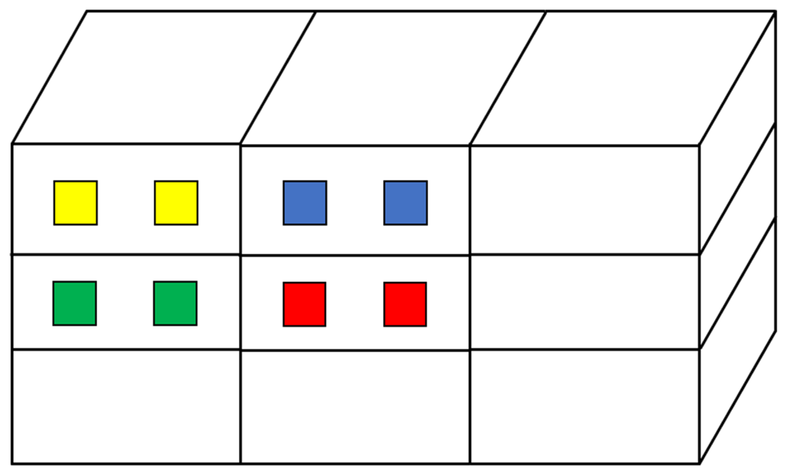
3.2. Pumping Airflow in Multi-Room Buildings

The pumping airflow of a multi-room building is analyzed in this section. The building model 2 is shown in Figure 20 with three rooms on each floor. There are a total of nine separate rooms, with a size of 18 m × 6 m × 9 m, and two openings on the leeward. The size of opening is 1 m × 1 m, and the distance between their center point is 3 m.

The size of the external computational domain is 186 m × 108 m × 9 m. The gridding, boundary conditions, turbulence model, discrete formatting, and parameter settings for simulation were identical to those in the aforementioned sections. The wind speed is assumed to be 1 m/s.

Considering the symmetry of the building model, four rooms were analyzed. The openings of the rooms were colored yellow, green, red, and blue, respectively, and these are called room 1, room 2, room 3, and room 4.

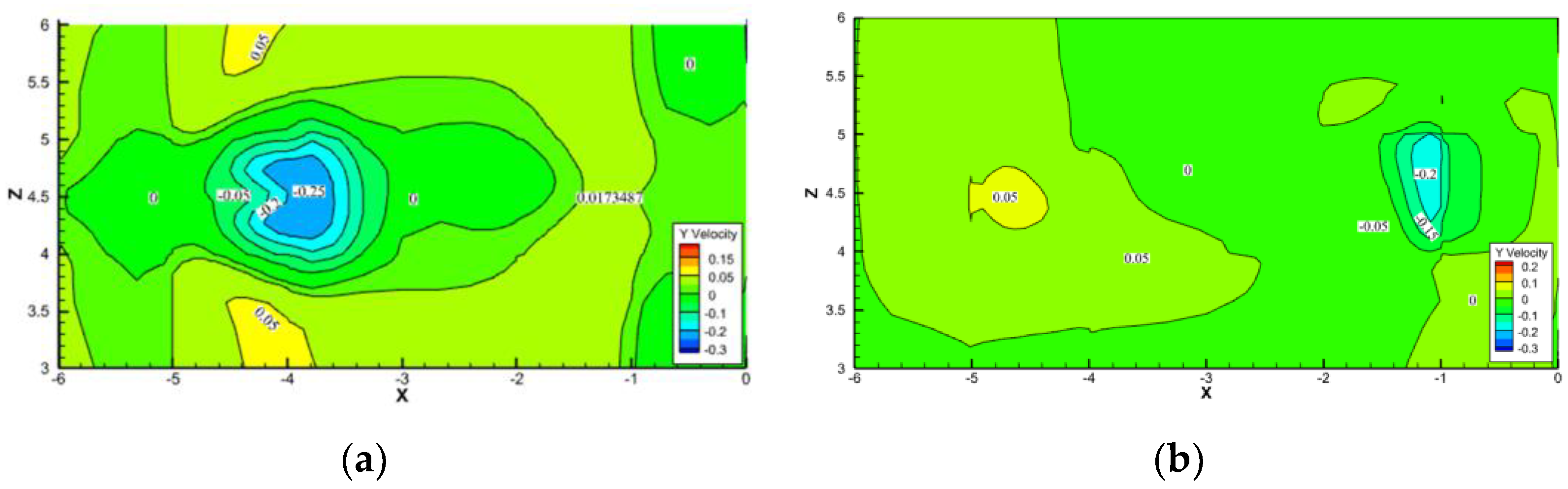
3.2.1. The Flow Characteristics

The simulation calculation settings in this section are the same as those in Section 2. The pumping flow characteristics are the same as well. However, the simulation results showed that the indoor airflow oscillation frequency was smaller than that of building 1 (0.0224 Hz); their values were 0.0073 Hz, 0.0075 Hz, 0.0075 Hz, and 0.0079 Hz, respectively.

The exterior flow fields of the single-room and multi-room building are depicted in Figure 21. It was possible to see that with the same incoming wind speed, the building body’s expansion caused a gradient increase in the velocity. In a result, a larger vortex formed and the velocity at the openings increased.

The indoor flow fields of the four rooms at t = 900 s are examined in Figure 22. It was discovered that for the side rooms (rooms 1 and 2), there was a greater difference in velocity magnitude at the openings, and the airflow entered the room at an angle to the windows; for the middle rooms 3 and 4, there was a smaller difference in velocity magnitude at the openings and the airflow flowed in and out of the windows almost parallel to the openings.

3.2.2. Ventilation Flow Rates

Table 9. Ventilation flow rates in different rooms.

Ventilation	Room 1	Room 2	Room 3	Room 4
$\mathrm{Dimensionless} \mathrm{average} \mathrm{ventilation} ({\overline{Q}}^{\prime }$)	0.2396	0.2479	0.3265	0.1917
$\mathrm{Dimensionless} \mathrm{fluctuations} \mathrm{ventilation} ({{\sigma }_Q}^{\prime }$)	0.1756	0.1946	0.3035	0.1350
Ventilation (m3/s)	0.1695	0.1753	0.2308	0.1356

lists the ventilation flow rates in the various rooms. According to the table, room 4 was the sole instance in which the dimensionless fluctuation ventilation flow rates are larger than the dimensionless mean value with a 20% difference. While the dimensionless fluctuating ventilation flow rates in rooms 1 and 2 were much less than the average value with differences of 36% and 27%, respectively, and the dimensionless average ventilation flow rates in room 3 were comparable to the fluctuating value with a difference of roughly 7%. The greatest value of the dimensionless fluctuating ventilation rate (room 4) was 1.3 times higher than the minimum value (room 1) in these four rooms, and the maximum value of the dimensionless mean ventilation rate (room 4) was 39% different from the lowest value (room 1).

In summary, room 1 had the lowest ventilation flow rate, while room 4 had the greatest. The reason is the vortex produced by the side walls of the building. Moreover, it can be seen from Table 9 that the ventilation flow rates of single-room buildings are smaller than those of multi-room buildings under the condition of same incoming wind speed and same building height. The reason may still be the flow split caused by the sidewall.

4. Conclusions

In this study, the pumping airflows of the single-room and the multi-room buildings were numerically simulated with an SST k-ω turbulent model, which was verified by an existing experiment. Through the unsteady simulation, the qualitative and the quantitative characteristics of the pumping ventilation were analyzed alongside the influence of the wind speed and the opening size. The primary conclusions are as follows.

(1)

For the pumping ventilation of the single-room buildings, the airflow direction at the leeward openings will change periodically. The ventilation flow rates also display the features of a regular fluctuation in a sine wave. Only the transient simulation can describe those flow characteristics. The vortex-shedding frequency is constant, which can be described in terms of the Ro number. For the case of this study, $Ro=0.098Re+4207.2$($4\times 10^5<Re<2.1\times 10^6$).

(2)

The airflow oscillation frequency is basically the same as the vortex-shedding frequency around the building; all of them vary monotonically with wind speed. As the wind speed increases, the frequency of the oscillations inside the building rise. The variation in the dimensionless opening spacing has an insignificant impact on the room’s airflow oscillation frequency.

(3)

The ventilation flow rates of the Warren model are not suitable for the pumping ventilation. However, the ventilation flow rates are also proportional to the wind speed and the opening areas. By fitting the simulation data, the formula for calculating the amount of pumped ventilation in a single-room building was derived as $Q=0.246U_R{{A_e}_f}_f$. Additionally, a linear relationship was found between the dimensionless opening distance and the dimensionless ventilation flow rate as $Q=0.4872U_R{{A_e}_f}_{f}s\prime$.

(4)

For multi-room buildings, the ventilation effects of various rooms are different. The room in the center of the building had a larger air change rate than the rooms on the sides of the structure. Moreover, the ventilation performance of any space in multi-room buildings is better than that in single-room buildings under the conditions of the same wind speed and the same building height.

The study can help engineers distinguish the ventilation effect of the pumping ventilation and even judge the different effects of the outdoor pollutants for various rooms. However, the research took the incoming wind speed as a constant value in every quasi-3D model. In a real project, the wind velocity will change with time, and the flow field will be affected by the ground. Moreover, the thermal stack effect also needs to be considered. The characteristics of the pumping ventilation will be more complex than those provided in this paper, all of which need to be further studied.

References

1. Visagavel, K.; Srinivasan, P. Analysis of single side ventilated and cross ventilated rooms by varying the width of the window opening using CFD. Sol. Energy 2009, 83, 2–5. [Google Scholar] [CrossRef]
2. Van Hooff, T.; Blocken, B.; Tominaga, Y. On the accuracy of CFD simulations of cross-ventilation flows for a generic isolated building: Comparison of RANS, LES and experiments. Build. Environ. 2017, 114, 148–165. [Google Scholar] [CrossRef]
3. Tao, T. Research on Airflow Characteristics and Thermal Comfort of Thermopressurised Naturally Ventilated Rooms. Ph.D. Thesis, Yangzhou University, Jiangsu, China, 2015. (In Chinese). [Google Scholar]
4. Chu, C.R.; Chiu, Y.H.; Tsai, Y.T.; Wu, S.L. Wind-driven natural ventilation for buildings with two openings on the same external wall. Energy Build. 2015, 108, 365–372. [Google Scholar] [CrossRef]
5. Warren, P. The analysis of single sided ventilation measurements. Air Infiltration Rev. 1986, 7, 3–5. [Google Scholar]
6. Straw, M.P. Computation and Measurement of Wind Induced Ventilation. Ph.D. Thesis, University of Nottingham, Nottingham, UK, 2000. [Google Scholar]
7. Daish, N.C.; da Graça, G.C.; Linden, P.F.; Banks, D. Impact of aperture separation on wind-driven single-sided natural ventilation. Build. Environ. 2016, 108, 122–134. [Google Scholar] [CrossRef]
8. Zhong, H.Y.; Zhang, D.D.; Liu, D.; Zhao, F.Y.; Li, Y.; Wang, H.Q. Two-dimensional numerical simulation of wind driven ventilation across a building enclosure with two free apertures on the rear side: Vortex shedding and “pumping flow mechanism”. J. Wind. Eng. Ind. Aerodyn. 2018, 179, 449–462. [Google Scholar] [CrossRef]
9. Zhong, H.Y.; Zhang, D.D.; Liu, Y.; Liu, D.; Zhao, F.Y.; Li, Y.; Wang, H.Q. Wind driven “pumping” fluid flow and turbulent mean oscillation across high-rise building enclosures with multiple naturally ventilated apertures. Sustain. Cities Soc. 2019, 50, 101619. [Google Scholar] [CrossRef]
10. Albuquerque, D.P.; Sandberg, M.; Linden, P.F.; da Graça, G.C. Experimental and numerical investigation of pumping ventilation on the leeward side of a cubic building. Build. Environ. 2020, 179, 106897. [Google Scholar] [CrossRef]
11. Zhong, H.Y.; Jing, Y.; Liu, Y.; Zhao, F.Y.; Liu, D.; Li, Y. CFD simulation of “pumping” flow mechanism of an urban building affected by an upstream building in high Reynolds flows. Energy Build. 2019, 202, 109330. [Google Scholar] [CrossRef]
12. Zhong, H.Y.; Jing, Y.; Sun, Y.; Kikumoto, H.; Zhao, F.Y.; Li, Y. Wind-driven pumping flow ventilation of highrise buildings: Effects of upstream building arrangements and opening area ratios. Sci. Total Environ. 2020, 722, 137924. [Google Scholar] [CrossRef]
13. Zhong, H.Y.; Lin, C.; Sun, Y.; Kikumoto, H.; Ooka, R.; Zhang, H.L.; Hu, H.; Zhao, F.Y.; Jimenez-Bescos, C. Boundary layer wind tunnel modeling experiments on pumping ventilation through a three-story reduce-scaled building with two openings. Build. Environ. 2021, 202, 108043. [Google Scholar] [CrossRef]
14. da Graca, G.C.; Albuquerque, D.P.; Sandberg, M.; Linden, P.F. Pumping ventilation of corner and single sided rooms with two openings. Build. Environ. 2021, 205, 108171. [Google Scholar] [CrossRef]
15. Kobayashi, T.; Sandberg, M.; Fujita, T.; Lim, E.; Umemiya, N. Simplified estimation of wind induced natural ventilation rate caused by turbulence for a room with minute wind pressure. Proc.-Roomvent Vent. 2018, 2018, 613–618. [Google Scholar]
16. Tominaga, Y.; Mochida, A.; Yoshie, R.; Kataoka, H.; Nozu, T.; Yoshikawa, M.; Shirasawa, T. AIJ guidelines for practical applications of CFD to pedestrian wind environment around buildings. J. Wind. Eng. Ind. Aerodyn. 2008, 96, 1749–1761. [Google Scholar] [CrossRef]
17. Yoshie, R.; Jiang, G.; Shirasawa, T.; Chung, J. CFD simulations of gas dispersion around high-rise building in non-isothermal boundary layer. J. Wind. Eng. Ind. Aerodyn. 2011, 99, 279–288. [Google Scholar] [CrossRef]
18. Liu, J.; Niu, J. CFD simulation of the wind environment around an isolated high-rise building: An evaluation of SRANS, LES and DES models. Build. Environ. 2016, 96, 91–106. [Google Scholar] [CrossRef]
19. Mou, B.; He, B.J.; Zhao, D.X.; Chau, K.W. Numerical simulation of the effects of building dimensional variation on wind pressure distribution. Eng. Appl. Comput. Fluid Mech. 2017, 11, 293–309. [Google Scholar] [CrossRef]
20. Jiang, Y.; Alexander, D.; Jenkins, H.; Arthur, R.; Chen, Q. Natural ventilation in buildings: Measurement in a wind tunnel and numerical simulation with large-eddy simulation. J. Wind. Eng. Ind. Aerodyn. 2003, 91, 331–353. [Google Scholar] [CrossRef]
21. Roshko, A. Experiments on the flow past a circular cylinder at very high Reynolds number. J. Fluid Mech. 1961, 10, 345–356. [Google Scholar] [CrossRef]
22. Monai, R. Wind tunnel experiments on vortex shedding frequency and end effects of square columns. Exp. Mech. 1994, 9, 6. (In Chinese) [Google Scholar]
23. Caciolo, M.; Stabat, P.; Marchio, D. Full scale experimental study of single-sided ventilation: Analysis of stack and wind effects. Energy Build. 2011, 43, 1765–1773. [Google Scholar] [CrossRef]
24. Ziarani, N.N.; Cook, M.J.; Freidooni, F.; O’Sullivan, P.D. The role of near-façade flow in wind-dominant single-sided natural ventilation for an isolated three-storey building: An LES study. Build. Environ. 2023, 235, 110210. [Google Scholar] [CrossRef]
Figure 1. The flow chart of the study.
Buildings 13 03066 g001
Figure 2. Building model 1 and computational domain.
Buildings 13 03066 g002
Figure 3. Schematic diagram of different opening distances.
Buildings 13 03066 g003
Figure 4. Schematic diagram of grid division.
Buildings 13 03066 g004
Figure 5. Monitoring lines for grid-independence verification.
Buildings 13 03066 g005
Figure 6. Airflow velocity distribution in the plane with Z = 4.5 m. (a) Y = 3 m. (b) Y = 9 m.
Buildings 13 03066 g006
Figure 7. Schematic diagram of wind tunnel experiment room.
Buildings 13 03066 g007
Figure 8. Validation of CFD methodology. (a) Schematic diagram of the location of wind tunnel experimental data measurements. (b) Numerical simulation of the velocity profile along the measurement line (red line) compared to the experimental values (black solid dots).
Buildings 13 03066 g008
Figure 9. Flow field of the building exterior. (a) Transient calculations. (b) Steady-state calculations.
Buildings 13 03066 g009
Figure 10. Velocity distribution on the vertical surface of the opening. (a) Transient calculations. (b) Steady-state calculations.
Buildings 13 03066 g010
Figure 11. Streamline distribution of the flow field. (a) Moment t. (b) Moment t + 1/2t. (c) Moment 2t.
Buildings 13 03066 g011
Figure 12. Time-range diagram of ventilation at U y = 1 m/s, s = 0.5.
Buildings 13 03066 g012
Figure 13. Time-range diagram of ventilation at U y = 1 m/s, s = 0.25.
Buildings 13 03066 g013
Figure 14. Schematic of the location of the different monitoring points.
Buildings 13 03066 g014
Figure 15. Time and frequency domain of static pressure at point a. (a) Time-domain spectrum. (b) Frequency spectrum.
Buildings 13 03066 g015
Figure 16. Linear relationship between Ro number and Re number.
Buildings 13 03066 g016
Figure 17. Time-domain plot of ventilation for two openings.
Buildings 13 03066 g017
Figure 18. Frequency of airflow oscillations in different locations with different wind speeds.
Buildings 13 03066 g018
Figure 19. The relationship of ventilation flow rates and wind speed.
Buildings 13 03066 g019
Figure 20. Schematic diagram and computational domain of the multi-room building.
Buildings 13 03066 g020aBuildings 13 03066 g020b
Figure 21. Velocity distribution of outdoor flow field in different buildings. (a) Single-room buildings (model 1). (b) Multi-room buildings (model 2).
Buildings 13 03066 g021
Figure 22. Velocity and streamline distribution of indoor flow field in different rooms in model 2. (a) Room 1. (b) Room 2. (c) Room 3. (d) Room 4.
Buildings 13 03066 g022