Influences of Heat Rejection from Split A/C Conditioners on Mixed-Mode Buildings: Energy Use and Indoor Air Pollution Exposure Analysis

Abstract

The heat rejected by outdoor units of split A/C conditioners can impact the ambient outdoor environment of mixed-mode buildings. Nevertheless, how this environmental impact may affect the space-conditioning energy use and indoor air pollution is poorly understood. By coupling EnergyPlus and Fluent, this study examines the effects of outdoor units’ heat rejection on the building surroundings, building cooling load, and indoor PM_2.5 exposure of a six-storey mixed-mode building. The building had an open-plan room on each floor, with the outdoor unit positioned below the window. The coupled model was run for a selected day when the building was cooled by air conditioning and natural ventilation. Five mixed-mode cooling strategies were simulated, reflecting different window-opening schedules, airflow rates of outdoor units, and cooling set-points. The results indicate that compared with the always-air-conditioned mode, the mixed-mode operation could significantly mitigate the negative impact of heat rejection on space-cooling energy consumption. Increasing the airflow rate of outdoor units led to a lower increase in demand for space cooling and lower indoor PM_2.5 exposure. If one of the six rooms needs to be cooled to a lower temperature than the others; choosing the bottom-floor room helped achieve more energy savings and better indoor air quality.

1. Introduction

In Hong Kong, split A/C conditioners are widely installed in buildings. A split A/C conditioner consists of a unit installed indoors and a unit installed outdoors. During cooling, outdoor units reject the heat from indoor units to outdoors. A building interacts with its ambient outdoor environment by heat convection between the ambient outdoor air and external surfaces, as well as by the exchange of air between the indoor and ambient outdoor environment of the building through ventilation and infiltration [1]. The outdoor air temperature can therefore significantly influence building energy consumption.

As the outdoor units’ heat rejection can significantly influence ambient outdoor temperatures, the heat rejection data have been incorporated in several studies on building energy use. Chow and Lin [2] used a modelling approach to investigate the temperature profile of the air within a tall building re-entrant where the outdoor units were located; the model outputs indicate (1) that the heat rejected by the outdoor units of lower-floor rooms caused an increase in the temperatures of the air around upper-floor rooms and (2) that there was a higher amount of energy required for air conditioning due to this temperature increase. Many attempts have been made to reduce the negative effects caused by heat rejection on the energy efficiency of buildings. Chow et al. [3] examined the impacts of different re-entrant shapes on the space-cooling energy demand of residential buildings and suggested that outdoor units should be installed in T-shaped re-entrants to achieve better cooling efficiency. Research by Nada and Said [4] investigated the cooling performance of outdoor units arranged in different ways in a building shaft and found the layout that was most effective in terms of reducing space-conditioning energy consumption.

The above studies have shown the impact of heat rejection on the energy efficiency of sealed air-conditioned buildings, where the occupants kept the air conditioning on and windows closed. There has been, however, little research looking at how heat rejection may modify the energy consumption of mixed-mode buildings, which rely on both air conditioning and window-assisted natural ventilation to maintain occupant thermal comfort while avoiding a significant energy cost for the air conditioning [5]. Motivated by the need to cut carbon emissions from the building sector, the government of Hong Kong has started to encourage the implementation of mixed-mode cooling for existing buildings [6]. The effectiveness of mixed-mode cooling, however, is highly dependent on the ambient outdoor air temperatures. Opening windows cannot always help maintain indoor air temperatures at an acceptable level if the difference in temperature between ambient outdoor air and indoor air is too small and can even result in an energy penalty if the temperature of the ambient outdoor air is higher than that of the indoor air [7].

Another potential problem with mixed-mode cooling lies in diminished indoor air quality. Outdoor air pollutants can infiltrate into buildings via external walls, roofs, and open windows and therefore influence the level of indoor air pollution exposure, which can have negative impacts on occupant health [8]. Consequently, ambient outdoor air pollution is highly related to the risk of health problems for people living in mixed-mode buildings.

There is a series of studies that analyse the characteristics of air pollutants around buildings. There have been both field studies [9,10,11] indicating that buildings with different locations (e.g., urban, rural, and roadside) experienced different levels of ambient outdoor air pollution and modelling studies [12,13,14] showing different levels of ambient outdoor air pollution for flats on different floors of the containing building. Keshavarzian et al. [15] investigated the influences that different building cross-section shapes might have on the dispersion of air pollutants near a single building. Cui et al. [16] used a modelling approach to look at how the layout of buildings in an urban street canyon could affect the dispersion of pollutants around buildings. Xiong and Chen [17] assessed the impact of horizontal sunshields on the ambient outdoor air pollutant concentrations of rooms with single-sided ventilation.

Whereas previous research has examined the way in which the concentration of ambient outdoor air pollutants was influenced by factors including the location, height, building geometrics, and urban street canyon, there has been little research on how heat rejected by outdoor units can modify the concentration of the air pollutants around buildings. The majority of outdoor units are operated to discharge hot air into the outdoor environment. The high volumes of discharged hot air are likely to influence the airflow near the building, thereby influencing the dispersion of air pollutants near the building. Although some studies [18,19,20] have looked at changes in the airflow patterns around buildings as a result of heat rejection, their focus was centred on the relationship between the airflow pattern and the cooling efficiency of outdoor units. The impact of heat rejection on the level of air pollutants around buildings is still poorly understood.

The literature review concluded that: (1) more attention should be paid to the effect of heat rejection from outdoor units on the performance of mixed-mode buildings, where the air conditioning can be switched off and windows can be open under favourable indoor–outdoor temperature differences and (2) the effect of heat rejection from outdoor units on the concentrations of air pollutants in the proximity of mixed-mode buildings remains unclear. The objectives of this study are to examine how heat rejection may influence the ambient air temperatures and ambient fine particle (also known as PM_2.5) concentrations of a mixed-mode building and how these influences will change the space-cooling demand and occupant exposure to indoor PM_2.5. The building energy modelling tool EnergyPlus [21] was employed to estimate the space-cooling demand and occupant exposure to indoor PM_2.5, whilst the CFD software Fluent 2021R1 [22] was employed to estimate the airflow patterns and the concentrations of outdoor PM_2.5 around the building. Several mixed-mode cooling strategies were simulated in order to demonstrate how ambient outdoor environmental conditions could vary according to control variables including the window-opening schedule, airflow rate of outdoor units, and the cooling set-point. By assessing the building performance under different mixed-mode cooling strategies, the ways in which a mixed-mode building can be operated to reduce energy consumption and improve occupant health are discussed.

2. Methodology

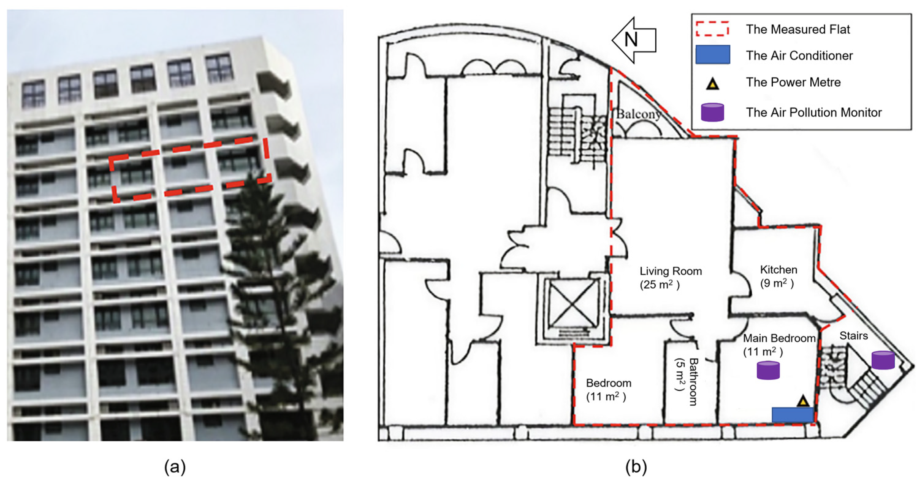
2.1. Building Model

The building model was run for a city block that had nine six-storey buildings (Figure 1a). The nine buildings were arranged in a layout of $3\times 3$ and were all identical in size, orientation, and construction. This type of city block is typical in the dense urban areas in Hong Kong according to the real estate data source [23]. The building in the middle was the mixed-mode building of interest. The building had an open-plan room (floor area: 80 m²; ceiling height: 3.4 m) on every floor, the exception being the ground floor. Each room had a south-oriented window, which had a height of 1.8 m and was 5.0 m in width. Stairs, lifts, and the ground-floor space (Figure 1b) were not included in the analysis. The surrounding buildings were treated as shading and wind-blocking components. The street canyon was 10 m in width. The model parameters, including the environmental conditions, fabrics, occupancy pattern, cooling system, and mixed-mode cooling strategies, are described below.

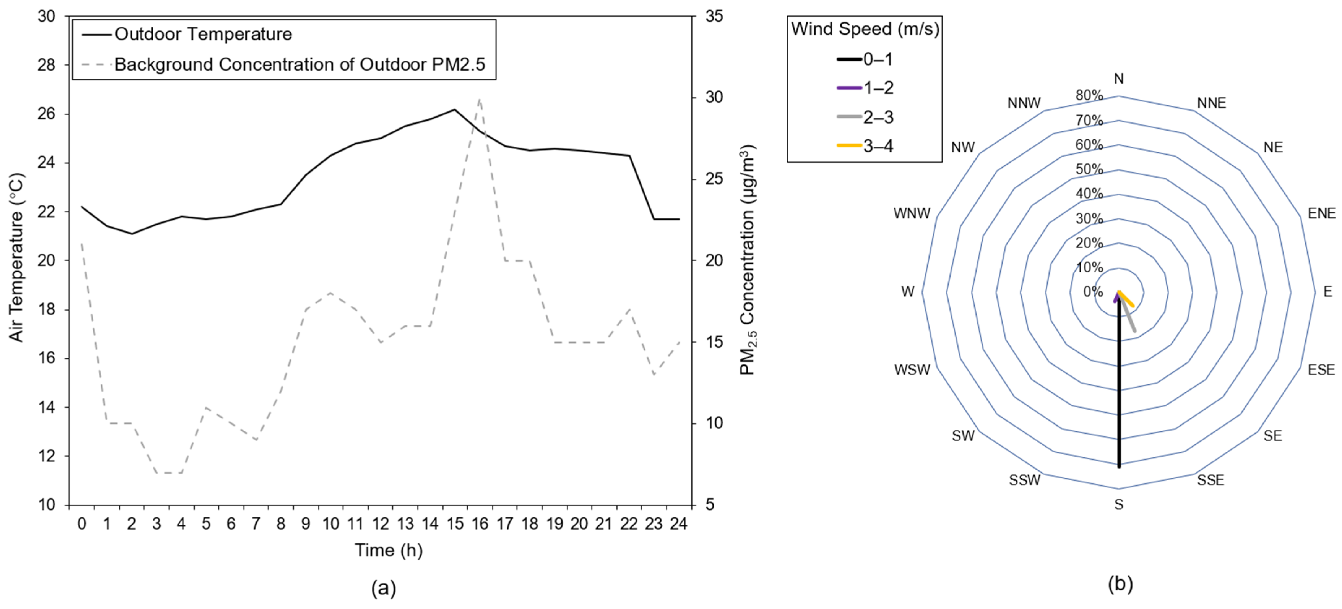
2.1.1. Environmental Conditions

Data on weather conditions were provided by the Hong Kong Observatory 2021 database [24]. Data on the background levels of outdoor PM_2.5 were provided by the Hong Kong EPD 2021 database [25]. The model was run for a three-day period during which the mixed-mode building was cooled using both air-conditioning and natural ventilation via open windows. The first two days were treated as “warmup days” in order to facilitate the convergence of results. The outdoor temperatures, wind speeds, wind directions, and background levels of outdoor PM_2.5 for the third day are shown in Figure 2. The mean values of the weather variables of the selected three-day period can represent the annual average weather conditions for Hong Kong. The advantage of using a three-day period is the reduction in computational costs, especially for the Fluent model. Given that the wind mainly blew from the south towards the north, a southerly wind was simulated for simplicity. In addition to the southerly wind, a northerly wind was simulated by only changing the wind direction without modifying the other weather parameters so as to demonstrate the impact of the wind direction.

2.1.2. Fabrics

This paper used an existing study [26] for the building envelope data (

Table 1. The materials and thermal characteristics of individual building fabrics.

Type	Materials	U-Value (W/m2K)	Solar Absorptance	Longwave Emission Coefficient	Solar Heat Gain Coefficient (SHGC)
External walls	Mosaic tiles (5 mm) + Cement (10 mm) + Heavy concrete (100 mm) + Gypsum plaster (10 mm)	3.1	Front: 0.4 Back: 0.5	Front: 0.9 Back: 0.9
Windows	Tinted glass (6 mm)	4.6			0.5
Roof	Concrete tiles (25 mm) + Asphalt (20 mm) + Cement (50 mm) + Polystyrene (50 mm) + Heavy concrete (150 mm) + Gypsum plaster (10 mm)	0.4	Front: 0.1 Back: 0.5	Front: 0.9 Back: 0.9
Ground floor	Floor tiles (10 mm) + Gypsum plaster (10 mm) + Reinforced concrete (180 mm)	3.0	Front: 0.8 Back: 0.5	Front: 0.9 Back: 0.9

). The thermal conductivity of each material was provided by the Buildings Department (BD) [27]. It was assumed that there was no exchange of heat between a room and its adjoining rooms. The airtightness of the building envelope was modelled using a permeability measurement (i.e., the rate of air leakage at 50 Pa indoor–outdoor pressure difference). The permeability was used to demonstrate the impact of different wind pressures on the infiltration rate. The infiltration rate of the building was first calculated using the ISO 13790 methodology [28] and then was changed into the permeability (11.5 m³/h/m²) based on the surface area and volume of the building.

2.1.3. Occupancy Pattern

The occupancy pattern determines both the internal heat gains and period of exposure. The number of occupants in individual rooms was set as seven to comply with the appropriate design occupation density for offices [29]. Occupants were assumed to be present from 08:00 to 15:00. The generation rates of the heat from people (130 W/person), lights (12 W/m²), and appliances (15 W/m²) were provided by CIBSE tables [29]. The occupancy pattern was overlaid on the profile of indoor PM_2.5 concentrations to determine occupant exposure to indoor PM_2.5.

2.1.4. Cooling Device

The cooling device in each room was modelled as a split A/C conditioner. The specification of the split A/C conditioner was taken from the engineering data provided by an A/C manufacturer [30]. The split A/C conditioner had a COP of 3.1. The outdoor unit, which took in air through the inlet on the back and discharged air through the outlet on the front, was positioned below the window of each room (Figure 1a). The air inlet and air outlet had areas of 1.1 m² and 0.9 m², respectively. To simplify analysis, the impact that the outdoor unit’s air intake might have on the airflow pattern near the building was ignored. The outdoor unit could be set up to operate at a high airflow rate of 85 m³/min or a low airflow rate of 65 m³/min.

2.1.5. Mixed-Mode Cooling Strategies

The mixed-mode building of interest was neither only naturally ventilated nor fully air-conditioned but relied on a combination of different energy-efficiency cooling techniques. The techniques used to cool each room included air conditioning and natural ventilation via an open window. Four air-conditioning patterns were considered, including:

• (all rooms 27 °C + low airflow rate): during occupied hours, all the rooms were cooled to a set-point of 27 °C. The outdoor units were set up to operate at a low airflow rate of 65 m³/min.
• (all rooms 27 °C + high airflow rate): during occupied hours, all the rooms were cooled to 27 °C. The outdoor units were set up to operate at a high airflow rate of 85 m³/min.
• (room five 23 °C and the rest 27 °C + low airflow rate): during occupied hours, the top-floor room (i.e., room 5) was cooled to 23 °C, whereas the rest were cooled to 27 °C. The outdoor units were set up to operate at a low airflow rate of 65 m³/min.
• (room one 23 °C and the rest 27 °C + low airflow rate): during occupied hours, room 1 (i.e., the room on the bottom floor) was cooled to 23 °C, whereas the rest were cooled to 27 °C. The outdoor units were set up to operate at a low airflow rate of 65 m³/min.

Two ventilation patterns were considered, including:

• (no window opening): all the windows in the building were closed. This reflects the ventilation pattern of a sealed air-conditioned building.
• (temperature-dependent window opening): a large indoor temperature swing can occur when the window was open, especially when there is a large indoor–outdoor temperature difference. This ventilation pattern aimed to comply with ASHRAE 55-2017 [31], which specifies that in order to reduce the negative impact of a large indoor temperature swing on occupant thermal comfort, the change in the temperature of the indoor air during a four-hour period should not exceed 3.3 °C. To meet the ASHRAE 55-2017 requirement, the temperatures inside and outside each room were calculated throughout the simulation period. When the difference in temperature between indoors and outdoors was in the range of 0 and ${\mathrm{T}}_{\mathrm{t}\mathrm{h}\mathrm{r}\mathrm{e}\mathrm{s}\mathrm{h}\mathrm{o}\mathrm{l}\mathrm{d}}$ , the window was open. When the indoor–outdoor delta temperature was larger than ${\mathrm{T}}_{\mathrm{t}\mathrm{h}\mathrm{r}\mathrm{e}\mathrm{s}\mathrm{h}\mathrm{o}\mathrm{l}\mathrm{d}}$, the window was closed. In both cases, the window was closed if the air conditioning was on, if natural ventilation was not able to keep indoor temperatures below the cooling setpoint, or if no one was in the room. The value of ${\mathrm{T}}_{\mathrm{t}\mathrm{h}\mathrm{r}\mathrm{e}\mathrm{s}\mathrm{h}\mathrm{o}\mathrm{l}\mathrm{d}}$ was determined via a series of simulations, with ${\mathrm{T}}_{\mathrm{t}\mathrm{h}\mathrm{r}\mathrm{e}\mathrm{s}\mathrm{h}\mathrm{o}\mathrm{l}\mathrm{d}}$ varying from 5.8 °C (i.e., the difference between the lowest temperature of the ambient outdoor air and the cooling set-point) to 0 in increments of −0.1 °C. Simulations stopped when the ASHRAE 55-2017 requirement was met; the value of ${\mathrm{T}}_{\mathrm{t}\mathrm{h}\mathrm{r}\mathrm{e}\mathrm{s}\mathrm{h}\mathrm{o}\mathrm{l}\mathrm{d}}$ was then determined.

Mixed-mode cooling strategies were developed by combining the air-conditioning and ventilation patterns described above. In total, there were five different mixed-mode cooling strategies to be simulated (

Table 2. The five different mixed-mode cooling strategies.

Mixed-Mode Cooling Strategy	Air-Conditioning Pattern	Ventilation Pattern
Strategy 1A	1 (all rooms 27 °C + low airflow rate)	A (no window opening)
Strategy 1B	1 (all rooms 27 °C + low airflow rate)	B (temperature-dependent window opening)
Strategy 2B	2 (all rooms 27 °C + high airflow rate)	B (temperature-dependent window opening)
Strategy 3B	3 (room five 23 °C and the rest 27 °C + low airflow rate)	B (temperature-dependent window opening)
Strategy 4B	4 (room one 23 °C and the rest 27 °C + low airflow rate)	B (temperature-dependent window opening)

).

2.2. Simulations

The building model described in Section 2.1 was developed in both EnergyPlus (v9.6) and Fluent (v2021-r1). EnergyPlus was applied to calculate cooling loads using the equation for heat balance, model the indoor airflow using the AirflowNetwork model, and calculate concentrations of indoor PM_2.5 using the generic contaminant transport algorithm. Fluent was applied to model the turbulent airflow near the building using the governing equations for incompressible airflow and calculate the concentrations of ambient outdoor PM_2.5 through a stochastic tracking approach. To ensure the accuracy of the input data (i.e., the temperatures of ambient outdoor air, ambient outdoor PM_2.5 concentrations, wind pressure coefficients, and temperatures of exterior surfaces), this study adopted a quasi-dynamic coupling method for EnergyPlus—Fluent co-simulation. The methods and assumptions used in the simulations are detailed below.

2.2.1. EnergyPlus Simulations

The outputs from Energyplus simulations included exterior surface temperatures, cooling loads, and concentrations of indoor PM_2.5. These variables were calculated at an interval of 10 min and output hourly.

The temperature of an exterior surface was calculated using the equation:

$${\mathrm{q}}_{\mathrm{a}\mathrm{s}\mathrm{o}\mathrm{l}}^{″}+{\mathrm{q}}_{\mathrm{L}\mathrm{W}\mathrm{R}}^{″}+{\mathrm{q}}_{\mathrm{c}\mathrm{o}\mathrm{n}\mathrm{v}}^{″}-{\mathrm{q}}_{\mathrm{k}\mathrm{o}}^{″}=0$$

(1)

where ${\mathrm{q}}_{\mathrm{a}\mathrm{s}\mathrm{o}\mathrm{l}}^{″}$ is the absorbed heat flux from solar radiation ($\mathrm{W}/{\mathrm{m}}^2$), ${\mathrm{q}}_{\mathrm{L}\mathrm{W}\mathrm{R}}^{″}$ is the exchange of long wavelength radiation flux with the air and the surroundings ($\mathrm{W}/{\mathrm{m}}^2$), ${\mathrm{q}}_{\mathrm{c}\mathrm{o}\mathrm{n}\mathrm{v}}^{″}$ is the exchange of convective flux with the outside air ($\mathrm{W}/{\mathrm{m}}^2$), and ${\mathrm{q}}_{\mathrm{k}\mathrm{o}}^{″}$ is the conduction heat flux ($\mathrm{W}/{\mathrm{m}}^2$).

The cooling load was estimated using the equation:

$${\mathrm{Q}}_{\mathrm{s}\mathrm{u}\mathrm{n}\_\mathrm{r}\mathrm{a}\mathrm{d}}+{\mathrm{Q}}_{\mathrm{i}\mathrm{n}\mathrm{t}\mathrm{e}\mathrm{r}\mathrm{n}\mathrm{a}\mathrm{l} \mathrm{s}\mathrm{u}\mathrm{r}\mathrm{f}\mathrm{a}\mathrm{c}\mathrm{e}\_\mathrm{r}\mathrm{a}\mathrm{d}}+{\mathrm{Q}}_{\mathrm{v}\mathrm{e}\mathrm{n}}+{\mathrm{Q}}_{\mathrm{i}\mathrm{n}\mathrm{f}}+{\mathrm{Q}}_{\mathrm{c}\mathrm{o}\mathrm{n}\mathrm{d}}+{\mathrm{Q}}_{\mathrm{i}\mathrm{n}\mathrm{t}\mathrm{e}\mathrm{r}\mathrm{a}\mathrm{l} \mathrm{h}\mathrm{e}\mathrm{a}\mathrm{t}}-{\mathrm{Q}}_{\mathrm{c}\mathrm{o}\mathrm{o}\mathrm{l}\mathrm{i}\mathrm{n}\mathrm{g}}=0$$

(2)

where ${\mathrm{Q}}_{\mathrm{s}\mathrm{u}\mathrm{n}\_\mathrm{r}\mathrm{a}\mathrm{d}}$ is the heat gain from solar radiation ($\mathrm{W}$), ${\mathrm{Q}}_{\mathrm{i}\mathrm{n}\mathrm{t}\mathrm{e}\mathrm{r}\mathrm{n}\mathrm{a}\mathrm{l} \mathrm{s}\mathrm{u}\mathrm{r}\mathrm{f}\mathrm{a}\mathrm{c}\mathrm{e}\_\mathrm{r}\mathrm{a}\mathrm{d}}$ is the transfer of radiative heat from the internal surfaces ($\mathrm{W}$), ${\mathrm{Q}}_{\mathrm{v}\mathrm{e}\mathrm{n}}$ is the ventilation heat gain ($\mathrm{W}$), ${\mathrm{Q}}_{\mathrm{i}\mathrm{n}\mathrm{f}}$ is the infiltration heat gain ($\mathrm{W}$), ${\mathrm{Q}}_{\mathrm{c}\mathrm{o}\mathrm{n}\mathrm{d}}$ is the conduction heat gain ($\mathrm{W}$), ${\mathrm{Q}}_{\mathrm{i}\mathrm{n}\mathrm{t}\mathrm{e}\mathrm{r}\mathrm{a}\mathrm{l} \mathrm{h}\mathrm{e}\mathrm{a}\mathrm{t}}$ is the occupant and equipment heat gain ($\mathrm{W}$), and ${\mathrm{Q}}_{\mathrm{c}\mathrm{o}\mathrm{o}\mathrm{l}\mathrm{i}\mathrm{n}\mathrm{g}}$ is the cooling load ($\mathrm{W}$).

According to the previous study [32], the heat rejection rate was calculated by adding up the energy required to cool the indoor space and the energy required for the A/C operation. The outlet air temperature of the outdoor unit was estimated using the equation:

$${\mathrm{T}}_{\mathrm{a}\mathrm{i}\mathrm{r}\_\mathrm{o}\mathrm{u}\mathrm{t}\mathrm{l}\mathrm{e}\mathrm{t}}=\frac{{\mathrm{Q}}_{\mathrm{r}\mathrm{e}\mathrm{j}\mathrm{e}\mathrm{c}\mathrm{t}\mathrm{e}\mathrm{d}}}{{\mathrm{M}}_{\mathrm{a}\mathrm{i}\mathrm{r}}{\mathrm{C}}_{\mathrm{p},\mathrm{a}\mathrm{i}\mathrm{r}}}+{\mathrm{T}}_{\mathrm{a}\mathrm{i}\mathrm{r}\_\mathrm{i}\mathrm{n}\mathrm{l}\mathrm{e}\mathrm{t}}$$

(3)

where ${\mathrm{Q}}_{\mathrm{r}\mathrm{e}\mathrm{j}\mathrm{e}\mathrm{c}\mathrm{t}\mathrm{e}\mathrm{d}}$ is the rate of heat rejection ($\mathrm{k}\mathrm{W}$), ${\mathrm{M}}_{\mathrm{a}\mathrm{i}\mathrm{r}}$ is the outdoor unit airflow ($\mathrm{k}\mathrm{g}/\mathrm{s}$), ${\mathrm{C}}_{\mathrm{p},\mathrm{a}\mathrm{i}\mathrm{r}}$ is the specific heat of air ($\mathrm{k}\mathrm{J}/\mathrm{k}\mathrm{g}·\mathrm{K}$), and ${\mathrm{T}}_{\mathrm{a}\mathrm{i}\mathrm{r}\_\mathrm{i}\mathrm{n}\mathrm{l}\mathrm{e}\mathrm{t}}$ is the temperature of the air at the inlet of the outdoor unit (°C).

The indoor level of outdoor-sourced PM_2.5 was determined using the generic contaminant model [33]. The outdoor-sourced PM_2.5 was modelled using a combination of PM_2.5 from vehicles and the background levels of outdoor PM_2.5 for Hong Kong (described in Section 2.1.1). The emission rate of PM_2.5 from vehicles in the street canyon (Figure 1c) was $1.13\times {10}^{-7} \mathrm{k}\mathrm{g}/\mathrm{s}$, according to a study on the air pollution caused by road traffic [34]. The ingress of the air from the ambient outdoor environment was modelled by assuming that there were cracks within the building fabrics (external walls, the roof and, when open, windows). The fraction of pollutant loss caused by the deposition of pollutants in the cracks (a.k.a. penetration factor) was set as 0.8 for closed windows and 1.0 for open windows [35]. Window opening was modelled assuming a two-way flow. The internal floors, ceilings, and walls were assumed to have cracks that allowed for the exchange of PM_2.5 between different rooms. The reference air mass flow coefficient of the cracks was assigned according to the area of the building surface and the permeability of the building envelope, with the exponent of air mass flow being 0.66 [36]. The rate of the deposition of outdoor-sourced PM_2.5 was set as $0.19 {\mathrm{h}}^{-1}$ [37]. It should be noted that the penetration rate and deposition rate of a particle are strongly related to the size of the particle; however, for simplicity, all the particles in this study were assumed to have the same size.

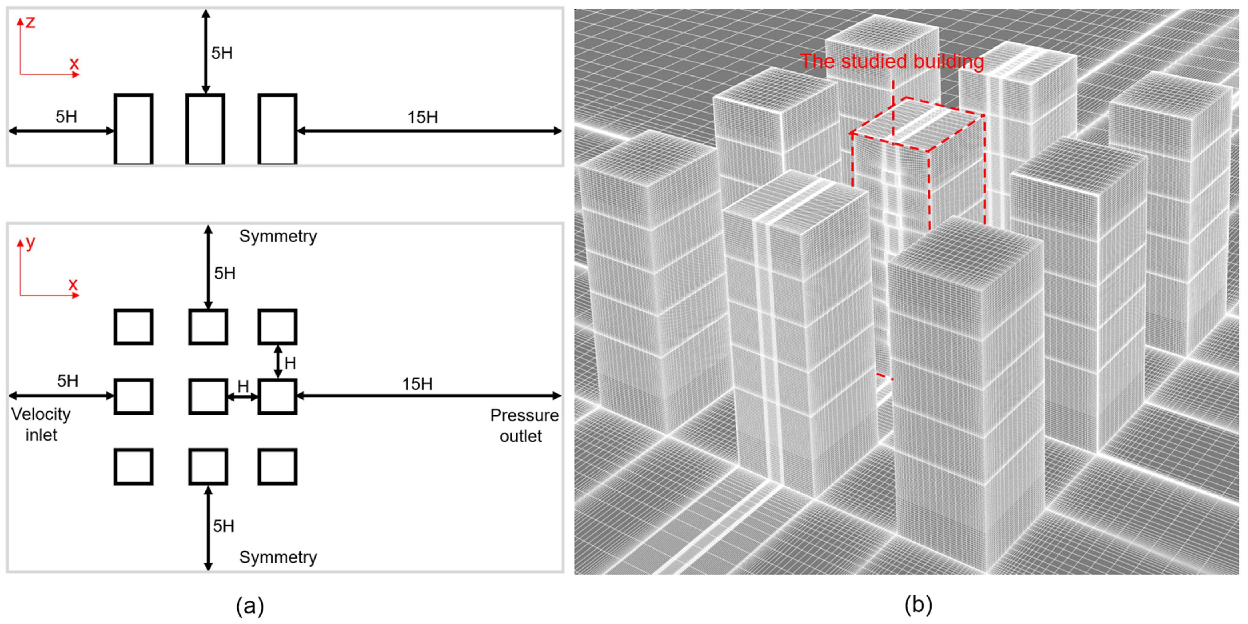
2.2.2. Fluent Simulations

The outputs from Fluent simulations included the temperature of the air around the building, concentration of PM_2.5 around the building, and coefficient of wind pressure. Data for these outputs were obtained from the grid layer that was closest to the building envelope.

The flow field was modelled using a three-dimensional standard k-ε model, which has frequently been used by similar studies because of its robustness and relatively low computing costs [38,39]. As in other similar research [16,40], the airflow was assumed to be numerically stable and was therefore incompressible turbulent. The general form of the governing equation for the airflow that is incompressible turbulent is written as:

$$\frac{\partial }{{\partial }_{\mathrm{t}}}\left(\partial \right)+\nabla ·\left({\overline{\mathrm{u}}}_{\partial }\right)-\nabla ·({\Gamma }_{\partial }{\nabla }_{\partial })={\mathrm{S}}_{\partial }$$

(4)

where $\overline{\mathrm{u}}$ is the average velocity, $\mathrm{S}$ is the source term, $\Gamma$ is the coefficient of effective diffusion, and $\partial$ is the scalar, which can be turbulent kinetic energy ($\mathrm{k}$), rate of dissipation ($\mathsf{\epsilon }$), or velocity ingredients.

The velocity–pressure coupling was solved using the SIMPLE algorithm. The second-order method was used to solve the pressure, convective, and diffusive terms. A standard wall function was assigned to the regions near walls. The time step of the simulation was 1 s. The number of iterations was kept below 600 for each time step. The convergence of results was obtained when the values of scaled residuals were less than ${10}^{-5}$ for the continuity equation and less than ${10}^{-6}$ for other equations.

The distribution of outdoor PM_2.5 was determined via a stochastic tracking method that estimates the particle trajectories by solving the balance of forces acting on the particle. The equation of the force balance for a particle is as follows:

$$\frac{\mathrm{d}{\mathrm{v}}_{\mathrm{p}}}{\mathrm{d}\mathrm{t}}={\mathrm{F}}_{\mathrm{d}}\left(\mathrm{v}-{\mathrm{v}}_{\mathrm{p}}\right)+\frac{{\mathrm{g}}_{\mathrm{x}}({\mathsf{\rho }}_{\mathrm{p}}-\mathsf{\rho })}{{\mathsf{\rho }}_{\mathrm{p}}}+{\mathrm{F}}_{\mathrm{a}\mathrm{d}\mathrm{d}}$$

(5)

where ${\mathrm{v}}_{\mathrm{p}}$ is the velocity of the particle, $\mathrm{v}$ is the velocity of air, ${\mathrm{F}}_{\mathrm{d}}\left(\mathrm{v}-{\mathrm{v}}_{\mathrm{p}}\right)$ is the drag force for every unit mass of the particle, ${\mathrm{g}}_{\mathrm{x}}$ is the acceleration due to gravity, ${\mathsf{\rho }}_{\mathrm{p}}$ is the density of the particle, $\mathsf{\rho }$ is the density of air, and ${\mathrm{F}}_{\mathrm{a}\mathrm{d}\mathrm{d}}$ is the additional acceleration term. No collision between particles was considered in this study.

A step-by-step report of particle trajectories was used to locate individual particles. The concentration of particles was determined using a particle-in-box approach. The equation for the particle-in-box approach is as follows:

$$\mathrm{C}=\frac{{\mathrm{M}}_{\mathrm{p}}{\sum }_{\mathrm{i}=1}^{\mathrm{n}}{\mathrm{N}}_{\mathrm{k}}^{\mathrm{i}}}{{\mathrm{V}}_{\mathrm{k}}}$$

(6)

where ${\mathrm{M}}_{\mathrm{p}}$ is the particle mass, ${\mathrm{N}}_{\mathrm{k}}^{\mathrm{i}}$ is the $\mathrm{i}$th particle that is in the box k, and ${\mathrm{V}}_{\mathrm{k}}$ is the volume of the box k.

As suggested by COST [41] and AIJ [42], a computational domain of the flow field (Figure 3a) was developed, with the inlet being 5H (H: the building’s height, which was 20 m) away from the city block, the outlet being 15H away from the city block, the sky being 5H away from the city block, and the lateral boundary being 5H away from the city block. To meet the size requirement of the validation carried out in Section 2.3, the entire model was scaled down by a factor of 25. For a reduced-scale model, the independence of the Reynolds number (${\mathrm{R}}_{\mathrm{e}}$) should be assessed [16]. The results of pre-simulations show that the ${\mathrm{R}}_{\mathrm{e}}$ values were $2.9\times {10}^5$ and $2.6\times {10}^5$ at building height and around outdoor units, respectively. Therefore, the independence requirement [43] that ${\mathrm{R}}_{\mathrm{e}}$ at the height of the building or around the envelope feature should be greater than $1.0\times {10}^4$ was met.

The structured grids within the city block (especially near buildings) were dense, whereas those in the surrounding regions were coarse (Figure 3b). The grid layer closest to the building surfaces, outdoor units, and ground was 0.001 m in height. This meshing strategy led to a mean $y^{\ast }$ of around 82, which was within the range of 30–300 required for a standard wall function [41]. To ensure there was a smooth transition in the size of the grids, the grids were drawn using an inflation ratio of no greater than 1.2.

An analysis of the grid sensitivity was conducted to keep the model outputs (including the normalised wind speeds and normalised PM_2.5 concentrations for ninety measurement points on the nominal vertical lines in the street canyon (Figure 1c)) independent of the grid size. The threshold for grid independence is that the root mean square error (RMSE) should be below 10%, as used in [15,44]. RMSE was determined using the equation:

$$\mathrm{R}\mathrm{M}\mathrm{S}\mathrm{E}=\sqrt{\frac{{\sum }_{\mathrm{i}=1}^{\mathrm{n}}{({\mathrm{y}}_{\mathrm{i}}-\widehat{{\mathrm{y}}_{\mathrm{i}}})}^2}{\mathrm{n}}}$$

(7)

where i is a measurement point up to $\mathrm{n}$ number of measurement points and ${\mathrm{y}}_{\mathrm{i}}$ and $\widehat{{\mathrm{y}}_{\mathrm{i}}}$ are the results of the measurement point i with two different grid configurations.

This study tested three different grid sizes (i.e., coarse, basic, and fine grids), with a refinement factor of 1.1 [41]. The number of cells for the coarse, basic, and fine grids were 1.9, 3.6, and 7.8 million, respectively. The results show that the RMSE between the coarse grids and basic grids was 23.1% and the RMSE between the basic grids and fine grids was only 4.6%. Therefore, the resolution of basic grids was considered sufficient and was applied to perform the validation performed in Section 2.3 and the parametric studies carried out in Section 3.

2.2.3. EnergyPlus and Fluent Co-Simulation

The quasi-coupling method was adopted for EnergyPlus–Fluent co-simulation. The coupling process is shown in Figure 4. First, EnergyPlus was run using the environmental data (shown in Section 2.1.1) to calculate the temperatures of the exterior surfaces and the outdoor units’ heat rejection rates. Then, Fluent was run using the outputs from EnergyPlus (including the temperatures of exterior surfaces and the rates of heat rejection) as boundary conditions to calculate temperatures of ambient outdoor air, concentrations of ambient outdoor PM_2.5, and coefficients of wind pressure. Finally, EnergyPlus was run using the modified environmental data that included the temperatures of ambient outdoor air and concentrations of ambient outdoor PM_2.5 output from Fluent to calculate the cooling loads, concentrations of indoor PM_2.5, temperatures of exterior surfaces, and heat rejected by outdoor units. The data exchange between EnergyPlus and Fluent was handled by Matlab 2020b [45] and took place every hour.

Table 3. Boundary conditions of the CFD domain during the coupling process.

Boundary	Type	Conditions
Ground	Wall	Non-slip; surface temperatures based on the meteorological data.
Building envelope	Wall	Non-slip; exterior surface temperatures outputted by EnergyPlus.
Sky and non-inlet/outlet laterals	Wall	Non-slip; adiabatic.
Domain inlet	Velocity inlet	Wind speed profile: ${\mathrm{U}}_{\mathcal{Z}}$; temperature profile: ${\mathrm{T}}_{\mathcal{Z}}$; turbulence kinetic energy profile: ${\mathrm{k}}_{\mathcal{Z}}$; and turbulence dissipation rate profile: ${\mathsf{\epsilon }}_{\mathcal{Z}}$.
Domain outlet	Pressure outlet	Gauge pressure of 0 pa; temperature profile ${\mathrm{T}}_{\mathcal{Z}}$; turbulence profiles: ${\mathrm{k}}_{\mathcal{Z}}$ and ${\mathsf{\epsilon }}_{\mathcal{Z}}$.
Outlet of the outdoor unit	Velocity inlet	Airflow rate: 65 or 85 m3/min; area of the air outlet: 0.9 m2; and temperature profile of ${\mathrm{T}}_{\mathrm{a}\mathrm{i}\mathrm{r}\_\mathrm{o}\mathrm{u}\mathrm{t}\mathrm{l}\mathrm{e}\mathrm{t}}$ (see Equation (3)).

summarizes the Fluent simulation’s boundary conditions.

It should be noted that ${\mathrm{U}}_{\mathcal{Z}}$ and ${\mathrm{T}}_{\mathcal{Z}}$ in Table 3 were calculated based on the following equations in order to match the wind speed and temperature patterns modelled in EnergyPlus:

$${\mathrm{U}}_{\mathrm{m}\mathrm{e}\mathrm{t}}{\left(\frac{{\mathsf{\delta }}_{\mathrm{m}\mathrm{e}\mathrm{t}}}{{\mathcal{Z}}_{\mathrm{m}\mathrm{e}\mathrm{t}}}\right)}^{{\mathsf{\alpha }}_{\mathrm{m}\mathrm{e}\mathrm{t}}}{\left(\frac{\mathcal{Z}}{\mathsf{\delta }}\right)}^{\mathsf{\alpha }}={\mathrm{U}}_{\mathcal{Z}}$$

(8)

$${\mathrm{T}}_{\mathrm{t}\mathrm{r}\mathrm{o}}+\frac{\mathrm{L}\mathrm{E}\mathcal{Z}}{\mathrm{E}+\mathcal{Z}}-\mathrm{L}{\mathrm{H}}_{\mathrm{t}\mathrm{r}\mathrm{o}}={\mathrm{T}}_{\mathcal{Z}}$$

(9)

$${\mathrm{T}}_{\mathrm{t}\mathrm{r}\mathrm{o}}={\mathrm{T}}_{\mathcal{Z},\mathrm{m}\mathrm{e}\mathrm{t}}-\mathrm{L}(\frac{\mathrm{E}{\mathcal{Z}}_{met}}{\mathrm{E}+{\mathcal{Z}}_{met}}-{\mathrm{H}}_{\mathrm{t}\mathrm{r}\mathrm{o}})$$

(10)

where ${\mathrm{U}}_{\mathrm{m}\mathrm{e}\mathrm{t}}$ is the measured velocity of the weather monitoring station ($\mathrm{m}/\mathrm{s}$), ${\mathsf{\delta }}_{\mathrm{m}\mathrm{e}\mathrm{t}}$ is the boundary layer thickness of the velocity profile of the weather monitoring station ($\mathrm{m}$), ${\mathcal{Z}}_{\mathrm{m}\mathrm{e}\mathrm{t}}$ is the height of the velocity sensor of the weather monitoring station ($\mathrm{m}$), ${\mathsf{\alpha }}_{\mathrm{m}\mathrm{e}\mathrm{t}}$ is the exponent of the velocity profile of the weather monitoring station, $\mathcal{Z}$ represents the altitude, $\mathsf{\delta }$ represents the thickness of the boundary layer of the velocity profile of the site, $\mathsf{\alpha }$ is the velocity profile exponent of the site, $\mathrm{L}$ is the air temperature gradient ($\mathrm{k}/\mathrm{m}$), $\mathrm{E}$ is the Earth radius, $\mathcal{Z}$ is the altitude, ${\mathrm{H}}_{\mathrm{t}\mathrm{r}\mathrm{o}}$ is the offset for the troposphere, ${\mathrm{T}}_{\mathrm{t}\mathrm{r}\mathrm{o}}$ is the ground-level air temperature for the troposphere (°C ), ${\mathrm{T}}_{\mathcal{Z},\mathrm{m}\mathrm{e}\mathrm{t}}$ is the measured outdoor air temperature of the weather station (°C ), and ${\mathcal{Z}}_{\mathrm{m}\mathrm{e}\mathrm{t}}$ is the height of the air temperature sensor of the weather station ($\mathrm{m}$).

The turbulence kinetic energy profile (${\mathrm{k}}_{\mathcal{Z}}$) mentioned in Table 3 was determined according to the following equation:

$${\mathrm{k}}_{\mathcal{Z}}=0.5\times ({\mathrm{u}}_{\mathrm{x},\mathcal{Z}}^{\prime 2}+{\mathrm{u}}_{\mathrm{y},\mathcal{Z}}^{\prime 2}+{\mathrm{u}}_{\mathrm{z},\mathcal{Z}}^{\prime 2})\cong 1.5\times {\mathrm{u}}_{\mathcal{Z}}^{\prime 2}$$

(11)

where ${\mathrm{u}}_{\mathrm{x},\mathcal{Z}}^{\prime }$, ${\mathrm{u}}_{\mathrm{y},\mathcal{Z}}^{\prime }$, and ${\mathrm{u}}_{\mathrm{z},\mathcal{Z}}^{\prime }$ are the root mean square of the velocity of the wind blowing in the x-axis, y-axis, or z-axis directions at a height of $\mathcal{Z}$ and ${\mathrm{u}}_{\mathcal{Z}}^{\prime }$ is the root mean square of the velocity of the streamwise wind at a height of $\mathcal{Z}$.

The turbulence dissipation rate profile (${\mathsf{\epsilon }}_{\mathcal{Z}}$) mentioned in Table 3 was determined according to the following equation:

$${\mathsf{\epsilon }}_{\mathcal{Z}}={\mathrm{C}}_{\partial }^{0.5}{\mathrm{k}}_{\mathcal{Z}}\frac{{\mathrm{U}}_{\mathrm{r}\mathrm{e}\mathrm{f}\mathrm{e}\mathrm{r}\mathrm{e}\mathrm{n}\mathrm{c}\mathrm{e}}}{{\mathcal{Z}}_{\mathrm{r}\mathrm{e}\mathrm{f}\mathrm{e}\mathrm{r}\mathrm{e}\mathrm{n}\mathrm{c}\mathrm{e}}}\mathsf{\alpha }{\left(\frac{\mathcal{Z}}{{\mathcal{Z}}_{\mathrm{r}\mathrm{e}\mathrm{f}\mathrm{e}\mathrm{r}\mathrm{e}\mathrm{n}\mathrm{c}\mathrm{e}}}\right)}^{\mathsf{\alpha }-1}$$

(12)

where ${\mathrm{C}}_{\partial }$ is the dimensionless constant of the standard k-ε model and ${\mathrm{U}}_{\mathrm{r}\mathrm{e}\mathrm{f}\mathrm{e}\mathrm{r}\mathrm{e}\mathrm{n}\mathrm{c}\mathrm{e}}$ is the reference velocity of the wind at a reference height of ${\mathcal{Z}}_{\mathrm{r}\mathrm{e}\mathrm{f}\mathrm{e}\mathrm{r}\mathrm{e}\mathrm{n}\mathrm{c}\mathrm{e}}$.

2.3. Validation

The simulation tools used herein were validated according to the results from the literature review and filed measurements. In Section 2.3.1 and Section 2.3.2, the grid size was determined according to the sensitivity analysis carried out in Section 2.2.2.

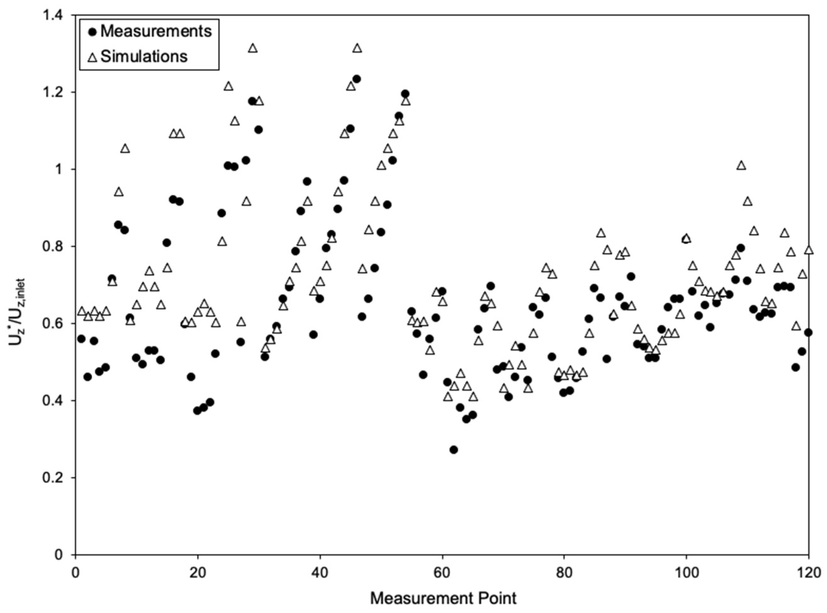
2.3.1. Airflow around Buildings

Data from a wind tunnel test carried out by the Architectural Institution of Japan (AIJ) [42] was used to assess the ability of Fluent to accurately model the flow field around buildings. In this wind tunnel test, nine cubes were arranged in a 3 × 3 array (Figure 5a). Each cube was 0.2 m in length. The street canyon was 0.2 m in width. As suggested by COST and AIJ (described in Section 2.2.2), the computational domain was developed using Fluent. The cube surface’s grid layer height was 0.003 m. The mean $y^{\ast }$ is about 75. The Fluent model used the boundary conditions of the wind tunnel test.

The measurement point (Figure 5b) heights were 0.02 m to measure velocities around cubes. The normalised velocity was equal to the ratio of the velocity of a point (${\mathrm{U}}_{\mathrm{z}}^{\ast }$) and the inflow velocity at the same height (${\mathrm{U}}_{\mathrm{z},\mathrm{i}\mathrm{n}\mathrm{l}\mathrm{e}\mathrm{t}}$). The comparison between measurements and simulations is shown in Figure 6. The average of the percentage differences (100% $\times$ (predicted value $-$ measured value)/measured value) was 15.5%, which shows a good match between the predicted and measured velocities.

In addition, the model accuracy was assessed based on three dimensionless metrics, which were the factor of 2 of observations ($\mathrm{F}\mathrm{A}\mathrm{C}2$), the fractional mean bias (FB), and the normalised mean square error ($\mathrm{N}\mathrm{M}\mathrm{S}\mathrm{E}$). The dimensionless metrics were calculated using:

$$\mathrm{F}\mathrm{A}\mathrm{C}2=\frac{1}{\mathrm{n}}\sum _{\mathrm{i}=1}^{\mathrm{n}}{\mathrm{n}}_{\mathrm{i}} \mathrm{w}\mathrm{i}\mathrm{t}\mathrm{h} {\mathrm{n}}_{\mathrm{i}}=\left\{\begin{array}{c}1,\mathrm{if} 0.5\le \frac{{\mathrm{s}}_{\mathrm{i}}}{{\mathrm{m}}_{\mathrm{i}}}\le 2\\ 1,\mathrm{i}\mathrm{f} {\mathrm{m}}_{\mathrm{i}}\le {\mathrm{W}}_{\mathrm{F}} \mathrm{and} {\mathrm{s}}_{\mathrm{i}}\le {\mathrm{W}}_{\mathrm{F}}\\ 0, \mathrm{else}\end{array}\right.$$

(13)

$$\mathrm{F}\mathrm{B}=\frac{2\times ({\sum }_{\mathrm{i}=1}^{\mathrm{n}}{\mathrm{m}}_{\mathrm{i}}-{\sum }_{\mathrm{i}=1}^{\mathrm{n}}{\mathrm{s}}_{\mathrm{i}})}{{\sum }_{\mathrm{i}=1}^{\mathrm{n}}{\mathrm{m}}_{\mathrm{i}}+{\sum }_{\mathrm{i}=1}^{\mathrm{n}}{\mathrm{s}}_{\mathrm{i}}}$$

(14)

$$\mathrm{N}\mathrm{M}\mathrm{S}\mathrm{E}=\frac{{\sum }_{\mathrm{i}=1}^{\mathrm{n}}{({\mathrm{m}}_{\mathrm{i}}-{\mathrm{s}}_{\mathrm{i}})}^2}{{\sum }_{\mathrm{i}=1}^{\mathrm{n}}{\mathrm{m}}_{\mathrm{i}}\times {\sum }_{\mathrm{i}=1}^{\mathrm{n}}{\mathrm{s}}_{\mathrm{i}}}$$

(15)

where ${\mathrm{n}}_{\mathrm{i}}$ is the $\mathrm{i}$th data point, $\mathrm{s}$ represents the simulation results, $\mathrm{m}$ represents the measurement results, and ${\mathrm{W}}_{\mathrm{F}}$ is the allowable absolute difference [46]. A CFD model that is acceptable for use in urban scenarios should meet the following requirements: $\mathrm{F}\mathrm{A}\mathrm{C}2\ge 0.3$, $-0.67\le \mathrm{F}\mathrm{B}\le 0.67$, and $\mathrm{N}\mathrm{M}\mathrm{S}\mathrm{E}\le 6$ [47,48]. The CFD model developed in this section met the criteria, as $\mathrm{F}\mathrm{A}\mathrm{C}2$ is 1, $\mathrm{F}\mathrm{B}$ is −0.1, and $\mathrm{N}\mathrm{M}\mathrm{S}\mathrm{E}$ is 0.03. Consequently, the final k-ε model in conjunction with the numerical setups could provide accurate estimates of the airflow patterns around buildings.

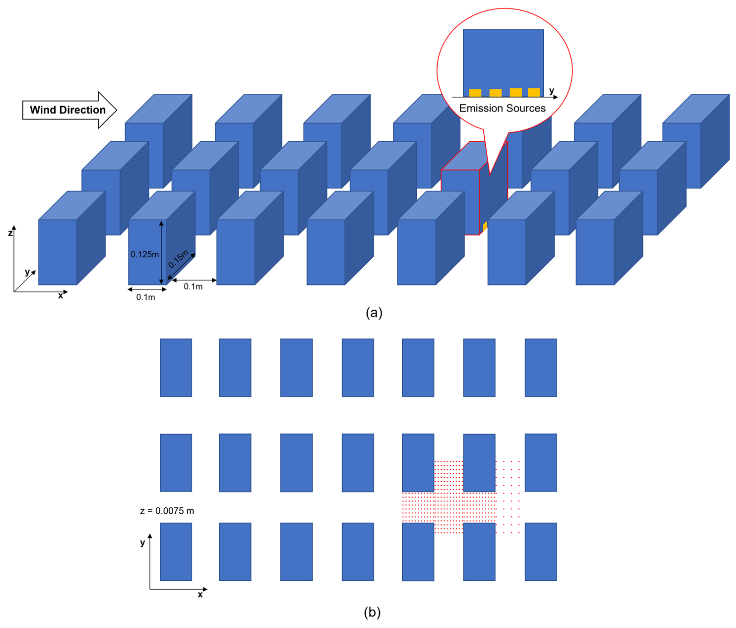
2.3.2. The Level of Air Pollution around Buildings

Data from a wind tunnel test carried out by the University of Hamburg [49] were used to assess the accuracy of ambient outdoor pollutant concentrations predicted by Fluent. In this wind tunnel test, 21 rectangular blocks (Figure 7a) were arranged in a 3 × 7 array. Each rectangular block had the same dimensions: 0.15 m length, 0.1 m width, and 0.125 m height. The street canyon was 0.1 m in width. The CFD domain was developed based on the suggestions from COST and AIJ (described in Section 2.2.2). Both the grid layers closest to the block surfaces and the ground have heights of 0.002 m (with $y^{\ast }$ being about 67). The boundary conditions of the wind tunnel test were applied to the Fluent model. The air pollutant emission source is the block’s bottom (Figure 7a). The emission velocity was 0.1 m/s, with the emission area being $4.6$ cm².

The study used 437 measurement points (Figure 7b) with heights of 0.0075 m for pollutant concentration measurements. The concentration values were normalised to a dimensionless K value that was calculated based on the equation:

$$\mathrm{K}=\frac{{\mathrm{C}}_{\mathrm{m}\mathrm{e}\mathrm{a}\mathrm{s}\mathrm{u}\mathrm{r}\mathrm{e}\mathrm{d}}{\mathrm{U}}_{\mathrm{r}\mathrm{e}\mathrm{f}}{\mathrm{H}}^2}{{\mathrm{C}}_{\mathrm{s}\mathrm{o}\mathrm{u}\mathrm{r}\mathrm{c}\mathrm{e}}{\mathrm{Q}}_{\mathrm{s}\mathrm{o}\mathrm{u}\mathrm{r}\mathrm{c}\mathrm{e}}}$$

(16)

where ${\mathrm{C}}_{\mathrm{m}\mathrm{e}\mathrm{a}\mathrm{s}\mathrm{u}\mathrm{r}\mathrm{e}\mathrm{d}}$ is the measured pollutant concentration (ppm), ${\mathrm{C}}_{\mathrm{s}\mathrm{o}\mathrm{u}\mathrm{r}\mathrm{c}\mathrm{e}}$ is the pollutant concentration of the emission source (ppm), ${\mathrm{U}}_{\mathrm{r}\mathrm{e}\mathrm{f}}$ is the measured reference velocity at a height of 0.66 m (m/s), $\mathrm{H}$ is the block height (m), and ${\mathrm{Q}}_{\mathrm{s}\mathrm{o}\mathrm{u}\mathrm{r}\mathrm{c}\mathrm{e}}$ is the emission rate of air pollutants (m³/s).

The comparison between the simulations and measurements is shown in Figure 8, which shows there was a good accuracy between the simulation and the measurement results. This conclusion was further supported by the metrics that reveal that $\mathrm{F}\mathrm{A}\mathrm{C}2$ is 1, $\mathrm{F}\mathrm{B}$ is −0.1, and $\mathrm{N}\mathrm{M}\mathrm{S}\mathrm{E}$ is 0.2. Consequently, the selected k-ε model and stochastic tracking model, in conjunction with the numerical setups, could provide reliable estimates of the pollutant concentrations within a city block.

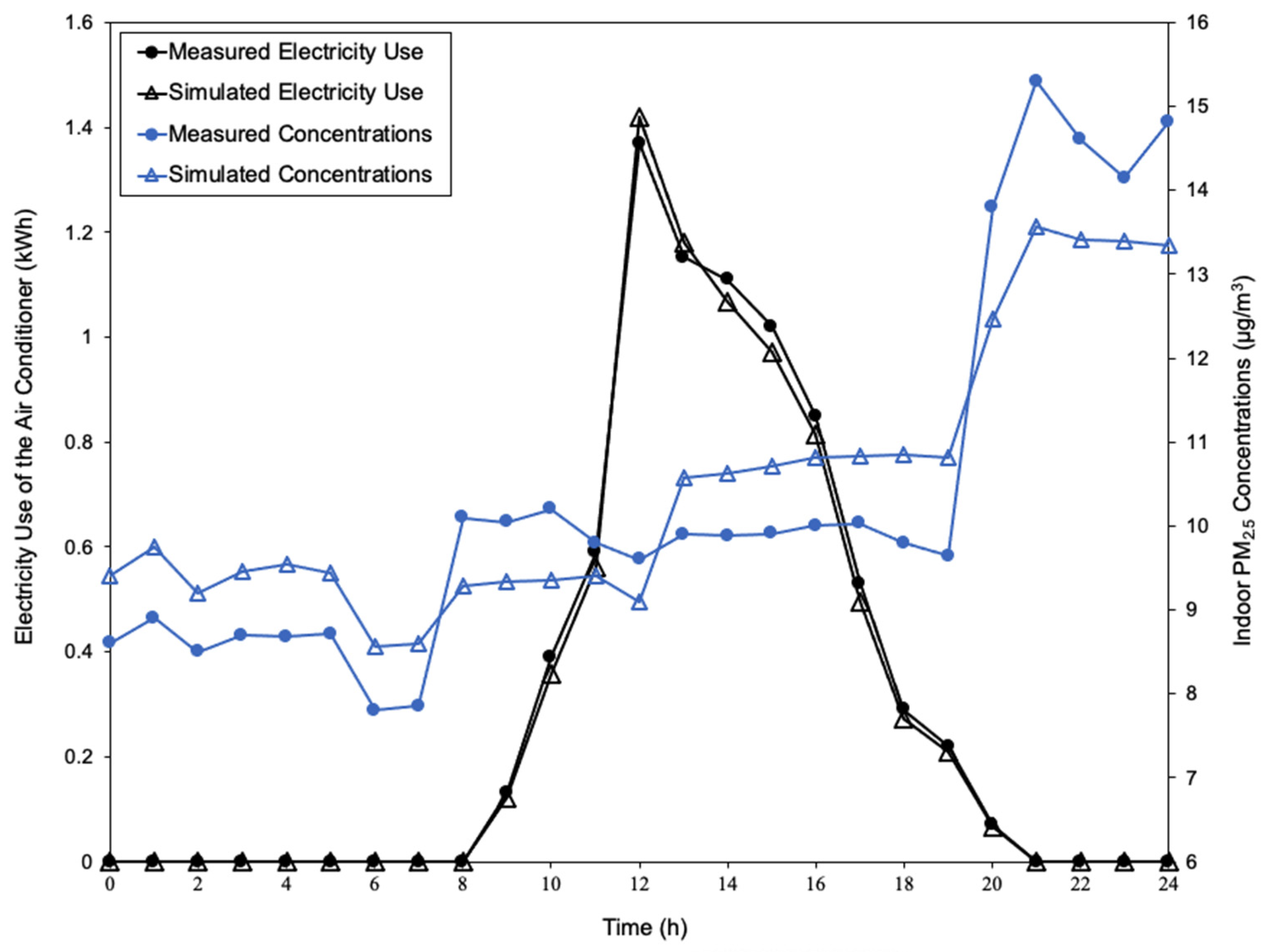
2.3.3. Space Cooling Demand and Indoor PM_2.5

Data from a field measurement was used to check the accuracy of space-cooling energy use and indoor pollutant levels predicted by EnergyPlus. A typical Hong Kong flat was used for field measurements (Figure 9a). The main bedroom of the flat had an air conditioner, with the COP being 2.4. The characteristics of the building fabrics were summarised as follows: (1) the rate of heat flow through the external walls, windows, roof, and ground floor were 3.1, 4.6, 0.42, and 0.54 $\mathrm{W}/{\mathrm{m}}^2\mathrm{K}$, respectively; (2) the window had a SHGC of 0.76; and (3) the airtightness of the building at 50 Pa was 10.1 ${\mathrm{m}}^3/\mathrm{h}/{\mathrm{m}}^2$. Windows and internal doors remained closed. During the measurement period, the air conditioner was run to maintain the indoor temperature of the main bedroom at 24 °C.

Measurements were taken from 28–30 September 2017. A power metre (SP2; BroadLink, Hangzhou, China) was applied to record the electric energy required to run the air conditioner in the main bedroom. The PM_2.5 level was measured via a calibrated air quality monitor (DUSTTRAK 8530 EP; TSI, Shoreview, MN, USA) that was accurate to ±5% and could measure the pollution level in the range from 0.001 $\mathrm{m}\mathrm{g}/{\mathrm{m}}^3$ to 150 $\mathrm{m}\mathrm{g}/{\mathrm{m}}^3$. The indoor PM_2.5 level was measured using the air quality monitor positioned in the middle of the main bedroom, whereas the outdoor PM_2.5 level was measured using the air quality monitor positioned on the stairs (Figure 9b). The nearby weather station (Kowloon City) data were used.

To understand the difference in results between measurements and simulations, the normalised mean bias error (NMBE) and the coefficient of variation of the root mean squared error (CVRMSE) were applied. ASHRAE Guideline 14-2014 [50] suggests that the simulation results are reliable if $\mathrm{N}\mathrm{M}\mathrm{B}\mathrm{E}<\pm 10\mathrm{\%}$ and $\mathrm{C}\mathrm{V}\mathrm{R}\mathrm{M}\mathrm{S}\mathrm{E}<30\mathrm{\%}$. The two errors were calculated as follows:

$$\mathrm{N}\mathrm{M}\mathrm{B}\mathrm{E}[\mathrm{\%}]=100\times \frac{{\sum }_{\mathrm{i}=1}^{\mathrm{n}}({\mathrm{y}}_{\mathrm{i}}-{{\mathrm{y}}_{\mathrm{i}}}^{\ast })}{\mathrm{n}\times \overline{\mathrm{y}}}$$

(17)

$$\mathrm{C}\mathrm{V}\mathrm{R}\mathrm{M}\mathrm{S}\mathrm{E}[\mathrm{\%}]=100\times \frac{\sqrt{{\sum }_{\mathrm{i}=1}^{\mathrm{n}}{({\mathrm{y}}_{\mathrm{i}}-{{\mathrm{y}}_{\mathrm{i}}}^{\ast })}^2/\mathrm{n}}}{\overline{\mathrm{y}}}$$

(18)

where $\mathrm{n}$ is the number of data points, $\mathrm{y}$ is the measurement result, ${\mathrm{y}}^{\ast }$ is the simulation result, and $\overline{\mathrm{y}}$ is the average of all the measurements.

An EnergyPlus model of the measured flat was constructed based on the geometry, building fabrics, air conditioner, weather conditions, and levels of outdoor PM_2.5 described above. Comparisons were made using the results for September 29, 2017. In general, the simulation results have good accuracy compared with the measurement results, as evidenced by Figure 10. The NMBE is 4.5% and the CVRMSE is 7.3%, which meets ASHRAE requirements. The simulated levels of indoor PM_2.5 were also in agreement with the measured ones, with the values of NMBE (8.5%) being less than 10% and CVRMSE (10.2%) being less than 30%. Consequently, the selected AirflowNetwork model and generic contaminant transport model, in conjunction with the numerical setups, could provide reliable estimates of energy demand for space-cooling and levels of indoor PM_2.5.

3. Results

The results presented herein show the ambient outdoor environmental conditions (i.e., temperatures, PM_2.5 concentrations, and airflow patterns), energy demand for space cooling, and indoor PM_2.5 exposure of the mixed-mode building operated using the cooling strategies described in Section 2.1.5. Based on the data taken from the surface shown in Figure 1d, the velocity vector, as well as the contours of temperatures and PM_2.5 concentrations, were drawn to help explain the results. A reference case with no heat rejected by the outdoor units was simulated so that variations in the surrounding outdoor environment because of heat rejection and the resulting changes in building performance could be estimated. There are two outdoor unit position scenarios: a leeward scenario, where the outdoor units are positioned on the leeward side, and a windward scenario, where the outdoor units are on the windward side (described in Section 2.1.1).

3.1. Ambient Outdoor Temperatures

Figure 11 shows the changes in the temperatures of the outdoor air around individual rooms due to heat rejection. The positive values represent that, compared with the reference case, the temperature increases.

3.1.1. Windward Scenario

Strategy 1A reflects those from previous modelling studies [17,18] examining the influence of heat rejection on the energy efficiency of sealed air-conditioned buildings, with heat rejection resulting in higher temperatures for the outdoor air around the building during the entire working period (Figure 11a). The increase in temperature for the outdoor air around individual rooms ranged from 0.1 °C to 1.4 °C. Averaged over the working hours, room 2 saw the greatest temperature increase. This was because whereas the hot air from each outdoor unit moved upwards because of the buoyancy effect, the conflict between the downward wind movement and the upward hot air movement kept the heat accumulated at second-floor height (Figure 12a). Room 5 saw the lowest temperature increase, since the downward wind took away the heat rejected by its outdoor unit (Figure 12a).

Compared with Strategy 1A, Strategy 1B shows that the temperature increase was eliminated or reduced at certain times during the working period (Figure 11b). No changes in the temperature of the outdoor air around individual rooms were observed from 08:00 to 11:00, during which all the outdoor units were switched off. During the period from 11:00 to 15:00, the increase in the temperature of the outdoor air around individual rooms was reduced to a range of 0.1 °C to 1.2 °C. This range was brought down further by Strategy 2B (Figure 11c), largely due to the fact that the outlet air temperature of the outdoor unit decreases as the airflow rate of the outdoor unit increases (according to Equation (1)).

When modelled under Strategy 3B, the temperature of the outdoor air around each room increased during the period from 08:00 to 11:00 (Figure 11d). This result is in line with Figure 12b. This is because the hot air from room 5’s outdoor unit was dispersed by the downward wind and caused the outdoor air temperature to increase around rooms 1 to 4. The results for Strategy 4B show that the temperature of the outdoor air around room 1 increased during the period from 08:00 to 11:00 (Figure 11e). This was caused by the trapped heat of the heat rejection from the outdoor unit of room 1 due to the downward wind (Figure 12c).

3.1.2. Leeward Scenario

The leeward scenario predicted an increase in the temperature of the outdoor air around individual rooms operating under Strategy 1A (Figure 11f). However, the leeward scenario shows a 1.6 °C greater temperature increase than the windward scenario. This result was because of two reasons: (1) under the windward scenario, wind dispersed part of the discharged heat (Figure 12a), and (2) under the leeward scenario, most of the heat was accumulated around the building (Figure 12d). The higher-floor rooms saw a higher temperature increase because the outdoor units’ rejected heat moved upwards.

For rooms 1 to 4, there was no significant difference between Strategy 1B and Strategy 3B on the temperature increase (Figure 11g,i). Room 5, on the other hand, saw a greater temperature increase under Strategy 3B than under Strategy 1B. This result was due to two factors: (1) more heat was rejected for room 5 as the cooling set-point was lower and (2) the rejected heat of room 5’s outdoor unit moved upwards (Figure 12e). An increase in the temperature of the outdoor air around individual rooms was predicted by Strategy 4B during the period from 08:00 to 11:00 (Figure 11j) because of the rejected heat of room 1’s outdoor unit moved upwards (Figure 12f). It should also be noted that under Strategy 4B, the outdoor unit of room 2 was switched on one hour earlier (10:00–11:00) because the hot air coming from the room 1’s outdoor unit caused higher ambient outdoor air temperatures.

3.2. Ambient Outdoor PM_2.5 Concentrations

The changes in the concentrations of outdoor PM_2.5 around individual rooms caused by heat rejection are shown in Figure 13, where the positive values represent higher concentrations compared with the reference case, whereas the negative values represent lower concentrations.

3.2.1. Windward Scenario

The results of Strategy 1A indicate a reduction in the concentrations of outdoor PM_2.5 around rooms 1 to 4 during the entire working period, with the average reduction for each room ranging from 0.8 $\mathsf{\mu }\mathrm{g}/{\mathrm{m}}^3$ to 10.6 $\mathsf{\mu }\mathrm{g}/{\mathrm{m}}^3$ (Figure 13a). This reduction was attributed in large part to the variation in the characteristics of the airflow within the street canyon. The air flow pattern at the bottom of the street canyon is affected when considering the hot air coming from outdoor units in the simulation. The airflow vortex was moved to the leeward side of the surrounding building (Figure 14a,b). This means that the fine particles released from the middle of the street canyon were prone to be blown to the surrounding buildings by the wind. A reduction in the levels of outdoor PM_2.5 around rooms 1 to 4 was predicted by Strategy 1B during the period from 11:00 to 15:00 (Figure 13b); this was again related to the movement of the airflow vortex at the street canyon’s bottom. Strategy 2B led to a greater reduction in the ambient outdoor PM_2.5 concentrations than Strategy 1B (Figure 13b,c), largely because the position of the airflow vortex was closer to the surrounding buildings, so the airflow rate of the outdoor units increased (Figure 14c).

The results of Strategy 3B show no obvious changes in the levels of outdoor PM_2.5 around the building (the exception being room 4, which saw a slight concentration decrease) during the period from 08:00 to 11:00 (Figure 13d). This was because of two reasons: (1) the heat rejection from room 5 was found to only change the pattern of the airflow near room 4 and room 5 (Figure 14e,f) and (2) the PM_2.5 from the middle of the street hardly moved to room 5 when there were no winds blowing them upwards. A reduction in the concentrations of outdoor PM_2.5 around rooms 1 to 4 could be seen under Strategy 4B during the period from 08:00 to 11:00 (Figure 13e). This was because the heat rejected by room 1 interfered with the upward wind that transported PM_2.5 from the street to the surroundings of the building (Figure 14g,h).

3.2.2. Leeward Scenario

The results of Strategy 1A show an increase in the concentration of outdoor PM_2.5 around room 1 and a reduction in the concentrations around rooms 2 to 5 during the entire working period (Figure 13f). When heat rejection was absent, PM_2.5 from the street was blown to the surroundings of individual rooms by the upward wind (Figure 14j). Above room 1’s outdoor unit there was a clockwise airflow vortex if heat rejection was considered in simulation (Figure 14i). This vortex could trap PM_2.5 that was transported by upward winds, resulting in an increase in the levels of outdoor PM_2.5 around room 1. Rooms 2 to 5 saw lower levels of ambient outdoor PM_2.5, likely attributable to more PM_2.5 from the street being contained near room 1. Similarly, higher levels of outdoor PM_2.5 around room 1 and lower levels of outdoor PM_2.5 around rooms 2 to 5 could be seen under Strategies 1B, 2B, and 3B during the period from 11:00 to 15:00 or under Strategy 4B during the entire working period (Figure 13g–j). When modelled under Strategy 3B, no change was seen in the concentrations of outdoor PM_2.5 around rooms 1 to 4 during the period from 08:00 to 11:00 (Figure 13i). However, during the same period, room 5 experienced higher ambient outdoor PM_2.5 concentrations due to the clockwise vortex above its outdoor unit (Figure 14d).

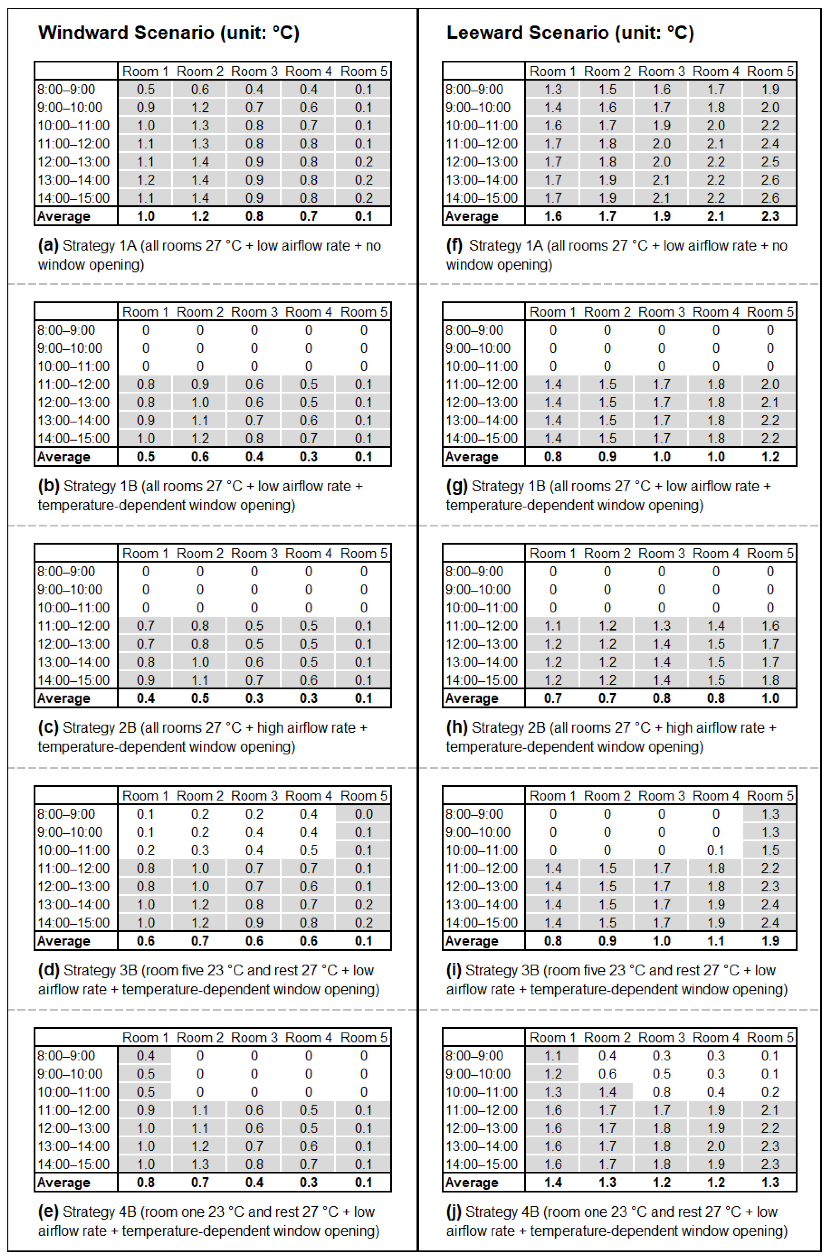
3.3. Cooling Loads

The building cooling loads were determined by summing the cooling loads of rooms 1 to 5. The changes in the building cooling loads due to heat rejection are shown in Figure 15, where the positive values represent higher cooling loads compared with the reference case.

3.3.1. Windward Scenario

As expected, the increased ambient outdoor temperatures described in Section 3.1.1 resulted in higher building cooling loads. Compared with Strategy 1A, Strategy 1B led to a 43.2% reduction in the increase in cooling loads (Figure 15). This result is in line with Figure 11a,b, showing that each room experienced lower ambient outdoor temperatures under Strategy 1B than under Strategy 1A. Similarly, the building cooling load predicted by Strategy 4B was 15.9% lower than that predicted by Strategy 3B (Figure 15) because of the increase in the temperature of outdoor air around rooms 2 to 5 being lower under Strategy 4B than under Strategy 3B (Figure 11d,e). Strategy 2B showed energy saving benefits, as the predicted building cooling load increase was 13.3% lower than Strategy 1B (Figure 15). This means increasing the airflow rate of outdoor units can improve energy efficiency.

3.3.2. Leeward Scenario

Higher outdoor temperatures meant greater building cooling loads, which is similar to the windward scenario. The trend between different strategies was: Strategy 1A resulted in the greatest cooling-load increase, followed Strategy 4B, then Strategy 3B, then Strategy 1B, and finally Strategy 2B (Figure 15). The cooling-load increase predicted by the windward scenario was on average 60.6% smaller than that predicted by the leeward scenario. The difference between Strategy 3B and Strategy 4B was the opposite of that observed under the windward scenario, with Strategy 3B leading to a 11.7% lower increase in cooling loads than Strategy 4B.

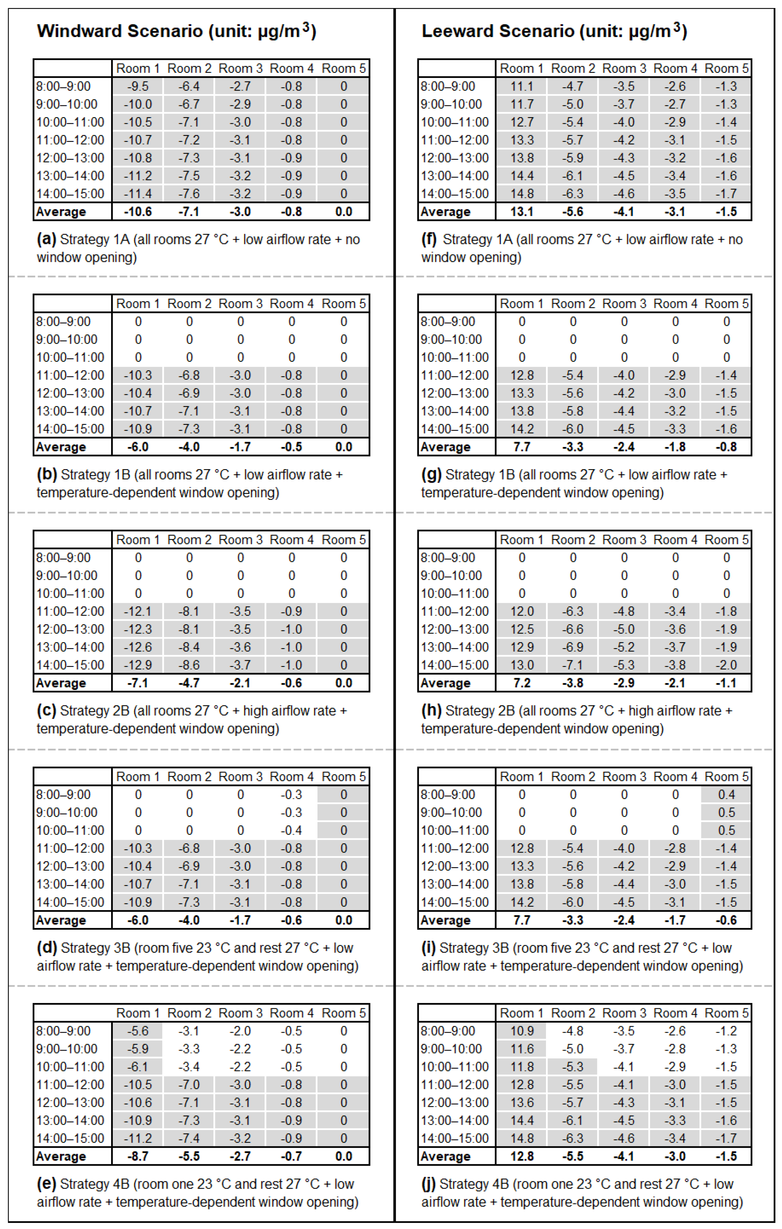
3.4. Indoor Levels of PM_2.5 Exposure

The results of exposure to indoor PM_2.5 were averaged over the working hours. Changes in the exposure of each room caused by heat rejection are shown in Figure 16, where the positive values represent a greater exposure in comparison with the reference case and the negative values represent lower exposures.

3.4.1. Windward Scenario

The results of Strategy 1A indicate that people in rooms 1 to 4 had reduced exposure to indoor PM_2.5 (Figure 16a), which was attributable to the reduced levels of ambient outdoor PM_2.5 (Figure 13a). No change in exposure was seen for room 5 (Figure 16a), as the concentrations of outdoor PM_2.5 around room 5 remained the same (Figure 13a). Compared with Strategy 1B, Strategy 2B led to lower indoor PM_2.5 exposures for rooms 1 to 4 (Figure 16a), showing the potential health benefit of increasing the airflow rates of outdoor units. Strategy 3B led to higher indoor PM_2.5 exposure than Strategy 4B (Figure 16a), mainly because the heat rejection from room 1 had a much stronger modifying effect on the concentrations of outdoor PM_2.5 around the building than the heat rejection room 5 (Figure 14e–h).

3.4.2. Leeward Scenario

Higher levels of indoor PM_2.5 exposure for room 1 were seen under each strategy (Figure 16b). This is because, as shown in (Figure 14i), there were greater concentrations of ambient outdoor PM_2.5 due to the formation of a vortex above the outdoor unit of room 1. People in rooms 2 to 5, on the other hand, experienced lower levels of indoor PM_2.5 exposure because of the reduction in the concentrations of outdoor PM_2.5 around rooms 2 to 5 (Figure 13f–j). Strategy 2B led to lower indoor PM_2.5 exposures for each room than Strategy 1B (Figure 16b), showing the potential health benefit of increasing the airflow rates of outdoor units.

4. Discussion

4.1. Main Findings

The simulation results indicate that the building had higher cooling loads because of the higher temperatures of ambient outdoor air due to heat rejection. This adverse energy effect varied in response to the wind direction, with simulation results showing that the cooling-load increase predicted by the windward scenario was 60.6% lower than that predicted by the leeward scenario. Under the leeward scenario, the heat rejected by the lower-level outdoor units could even result in the increased use of air-conditioning for rooms on higher levels. Averaged over the windward and leeward scenarios, the cooling-load increase due to heat rejection was 40.9% lower when windows were open based on temperature difference than when windows remained closed. This finding means that the influence of heat rejection on space-cooling energy consumption can vary significantly between sealed air-conditioned and mixed-mode buildings. Although an increase in the airflow rate of outdoor units could reduce the rate of ambient outdoor temperature increase due to heat rejection and thus lead to a smaller increase in cooling loads, this may not be possible in all buildings, for example those with concerns about noise. Additionally, the increased costs of running fans may reduce or even offset this energy benefit.

The position of the room that was cooled to a lower temperature than the others had a major influence on the cooling-load increase due to heat rejection, with the results of the windward scenario showing that the cooling-load increase predicted by Strategy 4B (room 1 being cooled to 23 °C and rooms 2 to 5 being cooled to 27 °C) was 15.9% lower than that predicted by Strategy 3B (room 5 being cooled to 23 °C and rooms 1 to 4 being cooled to 27 °C). The results for the windward scenario also indicate that Strategy 4B led to a lower indoor PM_2.5 exposure than Strategy 3B. An implication of these two findings is that under the windward scenario, an activity (e.g., meeting) that requires the indoor space to be cooled to a relatively low set-point temperature should take place in room 1 (i.e., the room on the bottom floor) rather than room 5 (i.e., the room on the top floor) in order to reduce space-conditioning energy consumption while improving indoor air quality.

Under the windward scenario, occupants experienced lower levels of exposure to indoor PM_2.5 since the heat rejection led to lower levels of ambient outdoor PM_2.5. The results for the leeward scenario show that occupants in room 1 faced higher levels of exposure to indoor PM_2.5 when heat rejection was present. In addition, it was found that the windward scenario led to lower cooling-load increases than the leeward scenario. Therefore, the location of outdoor units is a critical design decision. Outdoor units should be placed on the windward side of a building. Under both wind direction scenarios, higher airflow rates for outdoor units led to lower ambient outdoor PM_2.5 concentrations and thus contributed to better indoor air quality. Therefore, in addition to user preference, ease of installation, and cost, the decision to choose an outdoor unit may also come down to the rated airflow rate.

4.2. Limitations and Future Research

This study carries with it several limitations. Whereas the typical arrangement of outdoor units in Hong Kong was applied to the modelled building, future research on buildings that have different arrangements of outdoor units (e.g., outdoor units installed in re-entrants) is worth investigating. In addition, placing outdoor units on a single side is an important modelling simplification and must be acknowledged. Further work is ongoing to simulate the scenario that outdoor units are installed on both the windward and leeward sides. Previous studies [17,19] have suggested that the airflow pattern in a street canyon can change significantly between different aspect ratios. Further work is required to test more different aspect ratios to validate the sensitivity of the model. Indoor-sourced fine particles play an important role in indoor PM_2.5 exposure but are not considered herein. Heat rejection can influence the air exchange between the indoors and outdoors, thereby affecting the ability of indoor-sourced fine particles to exfiltrate. Fine particles from both indoor and outdoor sources will be modelled in future research. Outdoor units and envelope features such as external shading devices and balconies could be closely connected because they are usually positioned next to each other. The presence of external shading devices or balconies is likely to affect the flow pattern of the air discharged from outdoor units. Therefore, the combined effects of outdoor units and envelope features on the indoor environmental conditions should be investigated in future research.

Caution is also needed when generalising simulation results to the buildings that have the same geometrics as the modelled building. This study assigned a single orientation, a single occupancy pattern, and a single vertical profile of wind speeds to the model. However, it is acknowledged that variations in these model inputs may significantly influence the model outcomes. In terms of orientation, due to a greater exposure to the sun, a room with south-facing windows generally has higher indoor temperatures compared with its counterparts with non-south-facing windows [51]. This means that people in rooms with non-south-facing windows may air condition their rooms less frequently to maintain indoor thermal comfort. A decreased use of A/C can reduce the effects of heat rejection on space-cooling demands and indoor PM_2.5 exposure and thus influences the study results. The occupancy pattern determines both the internal heat gains and the periods when rooms are occupied and thus could have great impacts on space-cooling demands and indoor PM_2.5 exposure. The simulations were run based on an occupancy schedule representative of offices, and further research on whether similar results can be obtained from different occupancy schedules (e.g., household occupancy) is required. All simulations were run with a vertical profile of wind speeds that reflect a dense urban environment. The hot air discharged by outdoor units can influence the airflow pattern within the street canyon and therefore changes the conditions of the outdoor air around the building. The impact of the hot air on the airflow pattern within the street canyon, however, is likely to vary when wind speeds are modified to reflect a less dense urban environment.

5. Conclusions

By using a coupled EnergyPlus–Fluent modelling approach, this work has been able to investigate how heat rejection from outdoor units influenced the ambient outdoor environment of a mixed-mode building operating under different cooling strategies and how these influences affected space-cooling demands and indoor PM_2.5 exposure. The main outcomes of this study are:

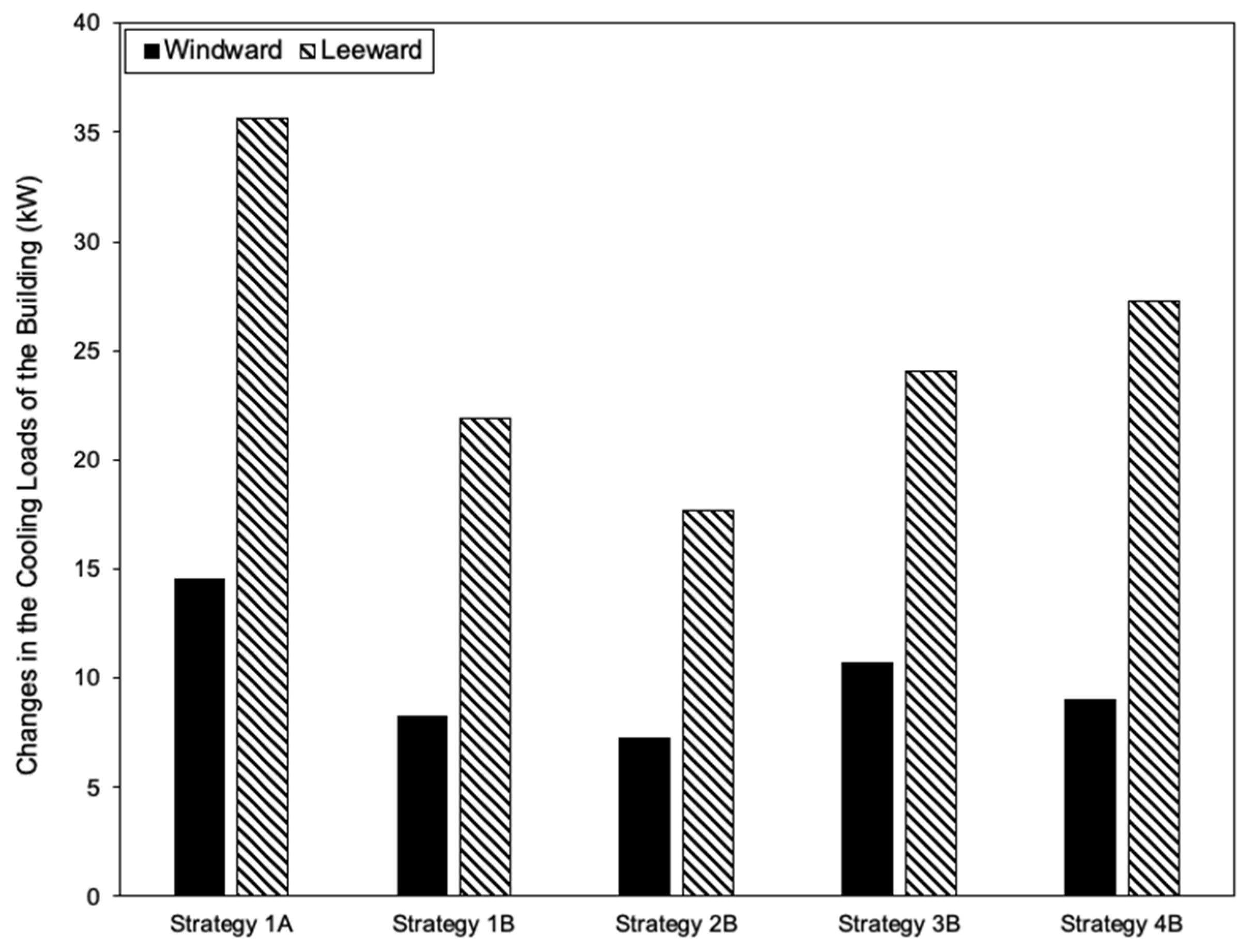
• The mixed-mode building had higher cooling loads because of the increase in ambient outdoor temperatures due to heat rejection. This adverse energy effect was more significant when windows remained closed than when windows were open based on temperature difference;
• Placing outdoor units on the windward side is beneficial to disperse the rejected heat from outdoor units, whereas the leeward scenario may “trap” the heat. Therefore, the windward scenario had 60.6% lower cooling load increase than the leeward scenario;
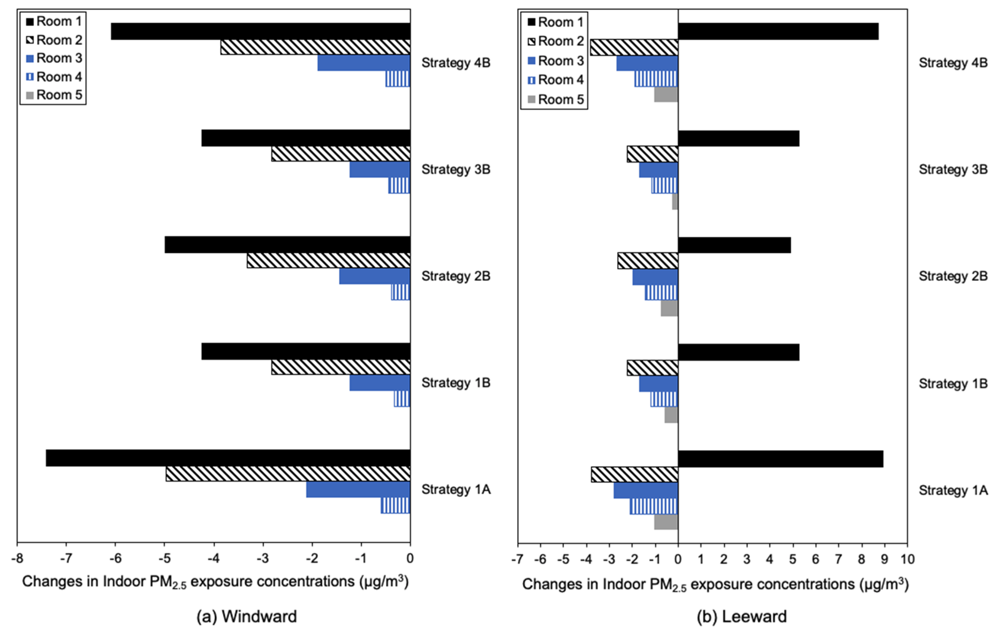
• In the windward scenario, PM_2.5 from the street was kept away from the buildings due to the airflow vortex generated by the heat rejection of the outdoor units, so the indoor PM_2.5 was lower. Under the leeward scenario, the bottom-floor room saw higher ambient outdoor PM_2.5 concentrations due to heat rejection; occupants in the bottom-floor room thus experienced greater exposure to indoor PM_2.5;
• The combination of outcomes (2) and (3) indicates that outdoor units should be placed on the windward side of a building in order to reduce both the space-cooling demands and exposure to indoor PM_2.5;
• An increase in the airflow rate of outdoor units offers the co-benefits of energy savings and occupant health under both the windward and leeward scenarios;
• Under the windward scenario, if one room needs to be cooled to a lower temperature than the others, the bottom-floor room is a better choice than the top-floor room for energy savings and occupant health.

References

- Hong, T.; Xu, Y.; Sun, K.; Zhang, W.; Luo, X.; Hooper, B. Urban microclimate and its impact on building performance: A case study of San Francisco. Urban Clim. 2021, 38, 100871. [Google Scholar] [CrossRef]
- Chow, T.T.; Lin, Z. Prediction of on-coil temperature of condensers installed at tall building re-entrant. Appl. Therm. Eng. 1999, 19, 117–132. [Google Scholar] [CrossRef]
- Chow, T.T.; Lin, Z.; Wang, Q.W. Effect of building re-entrant shape on performance of air-cooled condensing units. Energy Build. 2000, 32, 143–152. [Google Scholar] [CrossRef]
- Nada, S.A.; Said, M.A. Performance and energy consumptions of split type air conditioning units for different arrangements of outdoor units in confined building shafts. Appl. Therm. Eng. 2017, 123, 874–890. [Google Scholar] [CrossRef]
- Engelmann, P.; Kalz, D.; Salvalai, G. Cooling concepts for non-residential buildings: A comparison of cooling concepts in different climate zones. Energy Build. 2014, 82, 447–456. [Google Scholar] [CrossRef]
- Liu, S.; Kwok, Y.T.; Lau, K.K.-L.; Ouyang, W.; Ng, E. Effectiveness of passive design strategies in responding to future climate change for residential buildings in hot and humid Hong Kong. Energy Build. 2020, 228, 110469. [Google Scholar] [CrossRef]
- Bamdad, K.; Matour, S.; Izadyar, N.; Omrani, S. Impact of climate change on energy saving potentials of natural ventilation and ceiling fans in mixed-mode buildings. Build. Environ. 2022, 209, 108662. [Google Scholar] [CrossRef]
- Gens, A.; Hurley, J.F.; Tuomisto, J.T.; Friedrich, R. Health impacts due to personal exposure to fine particles caused by insulation of residential buildings in Europe. Atmos. Environ. 2014, 84, 213–221. [Google Scholar] [CrossRef]
- Jones, N.C.; Thornton, C.A.; Mark, D.; Harrison, R.M. Indoor/outdoor relationships of particulate matter in domestic homes with roadside, urban and rural locations. Atmos. Environ. 2000, 34, 2603–2612. [Google Scholar] [CrossRef]
- Canha, N.; Almeida, S.M.; Freitas, M.d.C.; Trancoso, M.; Sousa, A.; Mouro, F.; Wolterbeek, H.T. Particulate matter analysis in indoor environments of urban and rural primary schools using passive sampling methodology. Atmos. Environ. 2014, 83, 21–34. [Google Scholar] [CrossRef]
- Semmens, E.O.; Noonan, C.W.; Allen, R.W.; Weiler, E.C.; Ward, T.J. Indoor particulate matter in rural, wood stove heated homes. Environ. Res. 2015, 138, 93–100. [Google Scholar] [CrossRef] [PubMed]
- Taylor, J.; Davies, M.; Mavrogianni, A.; Shrubsole, C.; Hamilton, I.; Das, P.; Jones, B.; Oikonomou, E.; Biddulph, P. Mapping indoor overheating and air pollution risk modification across Great Britain: A modelling study. Build. Environ. 2016, 99, 1–12. [Google Scholar] [CrossRef]
- Taylor, J.; Shrubsole, C.; Symonds, P.; Mackenzie, I.; Davies, M. Application of an indoor air pollution metamodel to a spatially-distributed housing stock. Sci. Total Environ. 2019, 667, 390–399. [Google Scholar] [CrossRef] [PubMed]
- Taylor, J.; Shrubsole, C.; Davies, M.; Biddulph, P.; Das, P.; Hamilton, I.; Vardoulakis, S.; Mavrogianni, A.; Jones, B.; Oikonomou, E. The modifying effect of the building envelope on population exposure to PM2.5 from outdoor sources. Indoor Air 2014, 24, 639–651. [Google Scholar] [CrossRef] [PubMed]
- Keshavarzian, E.; Jin, R.; Dong, K.; Kwok, K.C.S. Effect of building cross-section shape on air pollutant dispersion around buildings. Build. Environ. 2021, 197, 107861. [Google Scholar] [CrossRef]
- Cui, D.; Li, X.; Liu, J.; Yuan, L.; Mak, C.M.; Fan, Y.; Kwok, K. Effects of building layouts and envelope features on wind flow and pollutant exposure in height-asymmetric street canyons. Build. Environ. 2021, 205, 108177. [Google Scholar] [CrossRef]
- Xiong, Y.; Chen, H. Effects of sunshields on vehicular pollutant dispersion and indoor air quality: Comparison between isothermal and nonisothermal conditions. Build. Environ. 2021, 197, 107854. [Google Scholar] [CrossRef]
- Hsieh, C.-M.; Aramaki, T.; Hanaki, K. Managing heat rejected from air conditioning systems to save energy and improve the microclimates of residential buildings. Comput. Environ. Urban Syst. 2011, 35, 358–367. [Google Scholar] [CrossRef]
- Adelia, A.S.; Yuan, C.; Liu, L.; Shan, R.Q. Effects of urban morphology on anthropogenic heat dispersion in tropical high-density residential areas. Energy Build. 2019, 186, 368–383. [Google Scholar] [CrossRef]
- Yuan, C.; Zhu, R.; Tong, S.; Mei, S.; Zhu, W. Impact of anthropogenic heat from air-conditioning on air temperature of naturally ventilated apartments at high-density tropical cities. Energy Build. 2022, 268, 112171. [Google Scholar] [CrossRef]
- Crawley, D.B.; Lawrie, L.K.; Winkelmann, F.C.; Buhl, W.F.; Huang, Y.J.; Pedersen, C.O.; Strand, R.K.; Liesen, R.J.; Fisher, D.E.; Witte, M.J.; et al. EnergyPlus: Creating a new-generation building energy simulation program. Energy Build. 2001, 33, 319–331. [Google Scholar] [CrossRef]
- Ansys, Inc. Ansys Fluids: Computational Fluid Dynamics (CFD) Simulation Software, version 2021; Ansys, Inc.: Canonsburg, PA, USA, 2021.
- EMPORIS. Building Types Hong Kong. 2017. Available online: https://www.emporis.com/city/101300/hong-kong-china (accessed on 16 September 2023).
- HKO. Climatological Information Services. 2021. Available online: https://www.hko.gov.hk/en/cis/climat.htm (accessed on 16 September 2023).
- EPD. Environmental Protection Interactive Centre: Air Quality Data—Download/Display. 2021. Available online: https://cd.epic.epd.gov.hk/EPICDI/air/station/?lang=en (accessed on 16 September 2023).
- Wan, K.S.Y.; Yik, F.H.W. Representative building design and internal load patterns for modelling energy use in residential buildings in Hong Kong. Appl. Energy 2004, 77, 69–85. [Google Scholar] [CrossRef]
- BD. Guidelines on Design and Construction Requirements for Energy Efficiency of Residential Buildings; Buildings Department Hong Kong: Hong Kong, China, 2014. [Google Scholar]
- ISO 13790; Energy Performance of Buildings, Calculation of Energy Use for Space Heating and Cooling. International Organization for Standardization (ISO): Geneva, Switzerland, 2008.
- CIBSE. CIBSE Guide A: Environmental Design; The Chartered Institution of Building Services Engineers: London, UK, 2006. [Google Scholar]
- Daikin. Engineering Data—Daikin AC; Daikin: Osaka, Japan, 2022. [Google Scholar]
- Standard 55-2017; Thermal environmental conditions for human occupancy. American Society of Heating, Refrigerating and Air Conditioning Engineers (ASHRAE): Peachtree Corners, GA, USA, 2017.
- Kikegawa, Y.; Genchi, Y.; Yoshikado, H.; Kondo, H. Development of a numerical simulation system toward comprehensive assessments of urban warming countermeasures including their impacts upon the urban buildings’ energy-demands. Appl. Energy 2003, 76, 449–466. [Google Scholar] [CrossRef]
- Taylor, J.; Shrubsole, C.; Biddulph, P.; Jones, B.; Das, P.; Davies, M. Simulation of pollution transport in buildings: The importance of taking into account dynamic thermal effects. Build. Serv. Eng. Res. Technol. 2014, 35, 682–690. [Google Scholar] [CrossRef]
- Meng, M.-R.; Cao, S.-J.; Kumar, P.; Tang, X.; Feng, Z. Spatial distribution characteristics of PM2.5 concentration around residential buildings in urban traffic-intensive areas: From the perspectives of health and safety. Saf. Sci. 2021, 141, 105318. [Google Scholar] [CrossRef]
- Taylor, J.; Mavrogianni, A.; Davies, M.; Das, P.; Shrubsole, C.; Biddulph, P.; Oikonomou, E. Understanding and mitigating overheating and indoor PM2.5 risks using coupled temperature and indoor air quality models. Build. Serv. Eng. Res. Technol. 2015, 36, 275–289. [Google Scholar] [CrossRef]
- Jones, B.; Das, P.; Chalabi, Z.; Davies, M.; Hamilton, I.; Lowe, R.; Milner, J.; Ridley, I.; Shrubsole, C.; Wilkinson, P. The Effect of Party Wall Permeability on Estimations of Infiltration from Air Leakage. Int. J. Vent. 2013, 12, 17–30. [Google Scholar] [CrossRef]
- Long, C.M.; Suh, H.H.; Catalano, P.J.; Koutrakis, P. Using Time- and Size-Resolved Particulate Data to Quantify Indoor Penetration and Deposition Behavior. Environ. Sci. Technol. 2001, 35, 2089–2099. [Google Scholar] [CrossRef]
- Liu, J.; Heidarinejad, M.; Pitchurov, G.; Zhang, L.; Srebric, J. An extensive comparison of modified zero-equation, standard k-ε, and LES models in predicting urban airflow. Sustain. Cities Soc. 2018, 40, 28–43. [Google Scholar] [CrossRef]
- Zhang, R.; Mirzaei, P.A.; Jones, B. Development of a dynamic external CFD and BES coupling framework for application of urban neighbourhoods energy modelling. Build. Environ. 2018, 146, 37–49. [Google Scholar] [CrossRef]
- Zheng, J.; Tao, Q.; Chen, Y. Airborne infection risk of inter-unit dispersion through semi-shaded openings: A case study of a multi-storey building with external louvers. Build. Environ. 2022, 225, 109586. [Google Scholar] [CrossRef] [PubMed]
- Franke, J.; Baklanov, A. Best Practice Guideline for the CFD Simulation of Flows in the Urban Environment: COST Action 732 Quality Assurance and Improvement of Microscale Meteorological Models; COST European Cooperation in Science and Technology: Hamburg, Germany, 2007. [Google Scholar]
- Tominaga, Y.; Mochida, A.; Yoshie, R.; Kataoka, H.; Nozu, T.; Yoshikawa, M.; Shirasawa, T. AIJ guidelines for practical applications of CFD to pedestrian wind environment around buildings. J. Wind Eng. Ind. Aerodyn. 2008, 96, 1749–1761. [Google Scholar] [CrossRef]
- Snyder, W. Guideline for Fluid Modeling of Atmospheric Diffusion; U.S. Environmental Protection Agency: Washington, DC, USA, 1981.
- Shirzadi, M.; Tominaga, Y. CFD evaluation of mean and turbulent wind characteristics around a high-rise building affected by its surroundings. Build. Environ. 2022, 225, 109637. [Google Scholar] [CrossRef]
- Gdeisat, M.; Lilley, F. 1—MATLAB® Integrated Development Environment. In Matlab by Example; Gdeisat, M., Lilley, F., Eds.; Elsevier: Amsterdam, The Netherlands, 2013; pp. 1–20. [Google Scholar] [CrossRef]
- Roache, P.J. Perspective: A Method for Uniform Reporting of Grid Refinement Studies. J. Fluids Eng. 1994, 116, 405–413. [Google Scholar] [CrossRef]
- Tominaga, Y.; Stathopoulos, T. CFD simulations of near-field pollutant dispersion with different plume buoyancies. Build. Environ. 2018, 131, 128–139. [Google Scholar] [CrossRef]
- Hanna, S.; Chang, J. Acceptance criteria for urban dispersion model evaluation. Meteorol. Atmos. Phys. 2012, 116, 133–146. [Google Scholar] [CrossRef]
- Leitl, B.; Schatzmann, M.C. Compilation of Experimental Data for Validation of Microscale Dispersion Models; Meteorological Institute of the University of Hamburg: Hamburg, Germany, 2010. [Google Scholar]
- Guideline 14–2014; Measurement of Energy, Demand, and Water Savings. American Society of Heating, Refrigerating, and Air Conditioning Engineers (ASHRAE): Peachtree Corners, GA, USA, 2014.
- Zhong, X.; Zhang, Z.; Wu, W.; Ridley, I. Comprehensive evaluation of energy and indoor-PM2.5-exposure performance of residential window and roller blind control strategies. Energy Build. 2020, 223, 110206. [Google Scholar] [CrossRef]