Evaluation of Moisture-Induced Stresses in Wood Cross-Sections Determined with a Time-Dependent, Plastic Material Model during Long-Time Exposure

Abstract

In recent years, the use of timber as a building material in larger construction applications such as multi-story buildings and bridges has increased. This requires a better understanding of the material to realize such constructions and design them more economically. However, accurate computational simulations of timber structures are challenging due to the complexity and inhomogeneity of this naturally grown material. It exhibits growth inhomogeneities such as knots and fiber deviations, orthotropic material behavior and moisture dependence of almost all physical parameters. Describing the creep response of wood under real climate conditions is particularly difficult. Changes in moisture content, plasticity and viscoelasticity affect moisture-induced stresses and potentially lead to cracks and structural damage. In this paper, we apply a material model that combines time and moisture-dependent behavior with multisurface plasticity to simulate cross-sections of different dimensions over a 14-month climate period. Our findings indicate that considering this long-term behavior has a minor impact on moisture-induced stresses during the drying period. However, during the wetting period, neglecting the time- and moisture-dependent material behavior of wood leads to a significant overestimation of tensile stresses within the cross-section, resulting in unrealistic predictions of wetting-induced fracture. Therefore, simulations during wetting periods require a sophisticated rheological model to properly reproduce the stress field.

1. Introduction

Change in moisture content (MC) is a critical factor that leads to damage in wood structures. A comprehensive investigation [1] examined a large dataset of 245 evaluations of damage in large-span timber structures. They found that in nearly half of the presented cases, damage correlates with a high or low MC, or significant variations in MC. Hence, accurate prediction of the moisture-dependent behavior is crucial for the design of timber structures. However, computational modeling of the naturally grown material wood is challenging due to its orthotropic and inhomogeneous structure. In addition, the hygroscopic behavior and time-dependency are observable in almost all material properties. Considering these effects in a numerical simulation requires either simplifying assumptions or comprehensive mathematical models.

The long-term mechanical processes in wood are still not fully researched, but comprehensive models describing the effects can be found in the literature. A review of the various models was recently presented in [2]. They summarized three mechanisms determining the creep deformation of wood: viscoelastic creep deformation at constant moisture content, which recovers completely when the load is removed [3]; mechanosorptive creep deformation that results from changes in the MC [3,4], which is recoverable and significantly outweighs the viscoelastic creep deformation; and irrecoverable mechanosorptive creep deformation associated with the maximum MC reached during analysis [5,6]. In addition, creep can be divided into three phases: primary, secondary, and tertiary creep [7]. Only primary creep, characterized by a decreasing creep rate, at a stress level below the “limit of linearity” exhibits linear viscoelasticity.

The existing literature provides a range of numerical implementations for wood creep models, varying in complexity. In [8], an Abaqus implementation is proposed following the mathematical description from [9], that includes mechanosorptive creep considered as permanent deformation [10]. Kelvin–Voigt elements were, to the best of the authors’ knowledge, initially proposed in [11]. In [3,12], this approach was extended by utilizing a series of Kelvin-Voigt elements to model linear viscoelastic creep. In this model, it was assumed that the stress levels remain below the limit of linearity. This allows for the superposition of individual load increments and simplifies the solution procedure of the posed problem. In [7,13], a model accounting for states past the limit of linearity is proposed. Nevertheless, many models still build on linear viscoelastic creep due to the ease of its implementation and good approximation capabilities. The model in [6] accounts for linear viscoelastic creep, linear mechanosorptive creep—through an additional series of Kelvin–Voigt elements—and irreversible mechanosorptive creep. The necessary creep coefficients were obtained by fitting to experimental results in [4,5]. An application of this model was shown in [14], where a glued laminated timber (GLT) beam was investigated during a 10-year time period. The material model from [6] was then further extended in [15] to include multisurface plasticity with hardening based on three failure surfaces specific to spruce wood.

An important consideration when modeling wood creep on the homogeneous orthotropic macroscopic level is the effect of the wood’s cellular structure and the composition of the cell wall material. As a result, the homogenized material behavior is directional dependent in both the time- and moisture-dependent properties [16]. This was, e.g., observed in [17] and is interpreted as a time-dependent Poisson’s ratio. In [16], a 2D rheological model for viscoelastic creep under constant climate conditions is proposed. Therein, the components of the creep compliance matrix scale differently from those of the elastic compliance matrix. This model was extended in [18] to 3D and updated to yield a symmetric creep compliance matrix. In [19,20], the capabilities of the model from [16] were investigated regarding mechanosorptive creep.

In this work, we study the effects of linear creep and plastic material behavior during long-time exposure of wood to realistic climate conditions. Recent research [21] revealed that simulating the wetting and drying of wood without considering mechanosorptive and viscoelastic creep as well as plasticity leads to an unrealistic formation of cracks in the interior of beams during the wetting period. A validated model for predicting the spatial MC below and above the fiber saturation point was presented in [22,23]. We used this model to determine the non-uniform time-dependent MC states in a wooden specimen. Subsequently, the specimen is analyzed under these predetermined states, accounting for linear viscoelastic creep, linear mechanosorptive creep, irreversible mechanosorptive creep, and multisurface plasticity. The material model is implemented in the commercial finite element software Abaqus 6.22-3 following the implementation from [6,15]. In contrast to this implementation, the multisurface failure criterion from [24] is used, which is based on a two-step homogenization strategy [25,26] accounting for material failure down to the cell wall. After the verification of the material model (in Section 3.1), the influence of the predetermined MC field (constant in Section 3.2 and non-uniform in Section 3.3) is shown. Finally, in Section 3.4, the long-term behavior of different-sized wooden cross-sections is investigated over a 14-month time span.

2. Materials and Methods

This section outlines the applied material models for simulating the moisture-dependent mechanical behavior of wood. While the mechanical response depends on the MC, the MC field can be determined independently of any state or solution fields of the mechanical problem. Hence, it is sufficient to consider the following sequentially coupled problem: First, a hygrothermal simulation (Section 2.1) is performed to determine the MC field. Following this, the MC field is used as a hygric load for the mechanical computation (Section 2.2). Both steps are performed using the finite element software Abaqus. Details on the implementation are provided in Appendix A.1.

2.1. Hygrothermal Multi-Fickian Transport Model

The hygrothermal model in [22] describes water transport in wood in three different phases: free water (which exists only above the fiber saturation point (FSP)), water vapor, and bound water. Furthermore, an energy conservation equation accounts for effects from the phase change processes as well as thermal conduction. These three phases are coupled through the process of evaporation or condensation, as well as sorption. During the studied 14-month time period, liquid water, e.g., rain, did not affect the wood cross-sections. Thus, the initial conditions are selected for a state below the FSP, allowing the free water phase to be disregarded. As shown in [21,23], this results in only three coupled differential equations. The material parameters used in this study match with the ones from [21,23].

The relationship between the water vapor content and the corresponding equilibrium-bound water content is characterized by the sorption isotherm. Based on such an isotherm and a bound water content-related reaction function, the sorption rate can be defined, describing the mass transfer between these two phases [27,28]. This can be based either on a single sorption isotherm for adsorption and desorption or separate sorption isotherms for each process. The latter case considers sorption hysteresis [29,30], which, in contrast to the single isotherm, leads, e.g., to higher MC values for desorption. Thus, sorption hysteresis affects the moisture-induced stresses and is used in the subsequent simulations unless stated otherwise.

2.2. Rheological Model for Wood

This section describes the mechanical material model, following the implementations from [6,15]. The six different, additively combined components of the total strain ${\mathit{\epsilon }}^{\mathrm{total}}$ are elastic ${\mathit{\epsilon }}^{\mathrm{el}}$, hygroexpansion ${\mathit{\epsilon }}^{\mathrm{u}}$, plastic ${\mathit{\epsilon }}^{\mathrm{p}}$, viscoelastic ${\mathit{\epsilon }}^{\mathrm{ve}}$, mechanosorptive ${\mathit{\epsilon }}^{\mathrm{ms}}$ and irrecoverable mechanosorptive ${\mathit{\epsilon }}^{\mathrm{ms},\mathrm{irr}}$ strain, thus,

$${\mathit{\epsilon }}^{\mathrm{total}}={\mathit{\epsilon }}^{\mathrm{el}}+{\mathit{\epsilon }}^{\mathrm{u}}+{\mathit{\epsilon }}^{\mathrm{p}}+\sum _{i=1}^p{\mathit{\epsilon }}_i^{\mathrm{ve}}+\sum _{j=1}^q{\mathit{\epsilon }}_j^{\mathrm{ms}}+{\mathit{\epsilon }}^{\mathrm{ms},\mathrm{irr}}.$$

(1)

The viscoelastic and mechanosorptive strains are composed of a series of Kelvin–Voigt elements with four elements in the case of viscoelasticity and three in the case of mechanosorption [6]. The following sections briefly describe these six components.

2.2.1. Elastic Strain

The elastic strain is assumed to be rate-independent [3]. Thus, it is explicitly defined by Equation (1), once all other strain components have been determined. Then, the corresponding stress tensor reads

$$\mathit{\sigma }={\mathit{C}}_0:{\mathit{\epsilon }}^{\mathrm{el}}={\mathit{C}}_0:\left({\mathit{\epsilon }}^{\mathrm{total}}-{\mathit{\epsilon }}^{\mathrm{u}}-{\mathit{\epsilon }}^{\mathrm{p}}-\sum _{i=1}^p{\mathit{\epsilon }}_i^{\mathrm{ve}}-\sum _{j=1}^q{\mathit{\epsilon }}_j^{\mathrm{ms}}-{\mathit{\epsilon }}^{\mathrm{ms},\mathrm{irr}}\right).$$

(2)

Herein, the moisture-dependent orthotropic compliance tensor ${\mathit{C}}_0^{-1}$, expressed in Voigt notation, is defined as

$${\mathit{C}}_0^{-1}=\left[\begin{array}{cccccc}\frac{1}{E_{\mathrm{L}}}& -\frac{{\nu }_{\mathrm{LR}}}{E_{\mathrm{R}}}& -\frac{{\nu }_{\mathrm{LT}}}{E_{\mathrm{T}}}& 0& 0& 0\\ -\frac{{\nu }_{\mathrm{LR}}}{E_{\mathrm{R}}}& \frac{1}{E_{\mathrm{R}}}& -\frac{{\nu }_{\mathrm{RT}}}{E_{\mathrm{T}}}& 0& 0& 0\\ -\frac{{\nu }_{\mathrm{LT}}}{E_{\mathrm{T}}}& -\frac{{\nu }_{\mathrm{RT}}}{E_{\mathrm{T}}}& \frac{1}{E_{\mathrm{T}}}& 0& 0& 0\\ 0& 0& 0& \frac{1}{G_{\mathrm{LR}}}& 0& 0\\ 0& 0& 0& 0& \frac{1}{G_{\mathrm{LT}}}& 0\\ 0& 0& 0& 0& 0& \frac{1}{G_{\mathrm{RT}}}\end{array}\right],$$

(3)

where

$$E_i=E_{i,\mathrm{ref}}\left(1+a(\rho -{\rho }_{\mathrm{ref}})+b(T-T_{\mathrm{ref}})+c(u-u_{\mathrm{ref}})\right)\mathrm{for} i\in \left\{\mathrm{L},\mathrm{R},\mathrm{T}\right\} \mathrm{and}$$

(4)

$$G_{ij}=G_{ij,\mathrm{ref}}\left(1+a(\rho -{\rho }_{\mathrm{ref}})+b(T-T_{\mathrm{ref}})+c(u-u_{\mathrm{ref}})\right)\mathrm{for} i,j\in \left\{\mathrm{L},\mathrm{R},\mathrm{T}\right\} \mathrm{with} i\ne j.$$

(5)

With the material parameters from [21,23], Equations (4) and (5) account for moisture dependence [8], where $a=0.0003{\mathrm{kg}}^{-1}{\mathrm{m}}^3$, $b=-0.007{\mathrm{K}}^{-1}$ and $c=-2.6$, with the reference Young’s moduli for the different directions $E_{\mathrm{L},\mathrm{ref}}=$ 10,000 MPa, $E_{\mathrm{R},\mathrm{ref}}=800$ MPa, $E_{\mathrm{T},\mathrm{ref}}=450$ MP as well as the reference shear moduli $G_{\mathrm{LR},\mathrm{ref}}=600$ MPa, $G_{\mathrm{LT},\mathrm{ref}}=650$ MPa and $G_{\mathrm{RT},\mathrm{ref}}=40$ MPa, the reference density ${\rho }_{\mathrm{ref}}=420\mathrm{kg}{\mathrm{m}}^{-3}$, the reference temperature $T_{\mathrm{ref}}=293.15$ K and the reference MC $u_{\mathrm{ref}}=0.12$. In contrast to [8], a density and temperature dependence of the stiffness parameters is not considered in this work. Poisson’s ratios are chosen as ${\nu }_{\mathrm{LR}}=0.027$, ${\nu }_{\mathrm{LT}}=0.033$ and ${\nu }_{\mathrm{RT}}=0.6$.

2.2.2. Hygroscopic Expansion

Hygroexpansion is assumed to be orthotropic, volumetric and constant. Thus, the expansion coefficient matrix $\mathit{\beta }$ consists of three non-zero diagonal entries of 0.015 for the longitudinal, 0.19 for the radial and 0.36 for the tangential direction. Based on the current MC u and the MC at the beginning of the analysis $u_{\mathrm{initial}}$ the hygroscopic expansion strain is determined as

$${\mathit{\epsilon }}^{\mathrm{u}}=\mathit{\beta }(u-u_{\mathrm{initial}}).$$

(6)

2.2.3. Irrecoverable Mechanosorption

Irrecoverable mechanosorption is driven by the maximum MC level reached during the simulation until the investigated point in time. As the MC at $t_{n+1}$ is known from the hygrothermal simulation preceding the mechanical simulation, ${\mathit{\epsilon }}^{\mathrm{ms},\mathrm{irr}}$ is determined according to [5,6] as

$$\Delta {\mathit{\epsilon }}^{\mathrm{ms},\mathrm{irr}}={\mathit{C}}_{\mathrm{ms},\mathrm{irr}}^{-1}:{\mathit{\sigma }}_n|\Delta \overline{U}|,$$

(7)

with ${\mathit{\sigma }}_n$ as the stress state at the beginning of the increment (following [31]), $|\Delta \overline{U}|$ as the incremental increase of the maximum reached MC level in the current time increment and the irrecoverable meachnosorptive compliance tensor

$${\mathit{C}}_{\mathrm{ms},\mathrm{irr}}^{-1}=\left[\begin{array}{cccccc}0& 0& 0& 0& 0& 0\\ 0& m_{\mathrm{v}}\frac{E_{\mathrm{T}}}{E_{\mathrm{R}}}& -m_{\mathrm{v}}\frac{E_{\mathrm{T}}{\nu }_{\mathrm{RT}}}{E_{\mathrm{R}}}& 0& 0& 0\\ 0& -m_{\mathrm{v}}\frac{E_{\mathrm{T}}{\nu }_{\mathrm{RT}}}{E_{\mathrm{R}}}& m_{\mathrm{v}}& 0& 0& 0\\ 0& 0& 0& m_{\mathrm{v}}\frac{E_{\mathrm{T}}}{G_{\mathrm{LR}}}& 0& 0\\ 0& 0& 0& 0& m_{\mathrm{v}}\frac{E_{\mathrm{T}}}{G_{\mathrm{LT}}}& 0\\ 0& 0& 0& 0& 0& m_{\mathrm{v}}\frac{E_{\mathrm{T}}}{G_{\mathrm{RT}}}\end{array}\right]$$

(8)

expressed in Voigt notation, with $m_{\mathrm{v}}=0.066$ ${\mathrm{MPa}}^{-1}$ according to [6]. Stress field contributions from mechanosorptive strains in the longitudinal direction are omitted in Equation (8), as this work focuses on studying effects in the radial–tangential plane of cross-sections. An alternative approach for the interpretation of $|\Delta \overline{U}|$ was presented in [2]. Therein, it is considered as load-phase-dependent, i.e., parts of the irrecoverable mechanosorptive MC are recovered during changes in external loading. This adaption resulted in a better fit of the presented experimental data.

2.2.4. Viscoelasticity

It is well established by experiments and theoretical considerations, that the Poisson’s ratio for wood is time-dependent. The models mentioned in Section 1 account for this, however, the large amount of additional viscoelastic and mechanosorptive material parameters are missing physical interpretability and require empirical determination. In this work, we rely on a model where the creep compliance matrix components are scaled in accordance with the components of the elastic compliance matrix. This requires fewer parameters and allows the use of a set of material parameters from the literature, that is already extensively validated.

Therefore, viscoelasticity is modeled with a series of four Kelvin–Voigt elements with retardation times ${\tau }_i$ between 2.4 h and 2400 h. Each Kelvin–Voigt element is described by the equation

$${\dot{\mathit{\epsilon }}}_i^{\mathrm{ve}}+\frac{1}{{\tau }_i}{\mathit{\epsilon }}_i^{\mathrm{ve}}=\frac{1}{{\tau }_i}{\mathit{C}}_{\mathrm{ve},i}^{-1}:\mathit{\sigma }\left(t\right).$$

(9)

This differential equation can be solved using the Laplace transform as mentioned in [2]. In case of creep, the initial stress $\mathit{\sigma }\left(0\right)$ and strain ${\mathit{\epsilon }}_i^{\mathrm{ve}}\left(0\right)$ are 0. ${\mathit{C}}_{\mathrm{ve},i}^{-1}$ and ${\tau }_i$ are assumed to be constant. Replacing

$$\begin{array}{cc}\hfill {\mathit{\epsilon }}_i^{\mathrm{ve}}& \mathrm{by}\mathit{X}\left(s\right),\hfill \\ \hfill {\dot{\mathit{\epsilon }}}_i^{\mathrm{ve}}& \mathrm{by}s\mathit{X}\left(s\right)-{\mathit{\epsilon }}_i^{\mathrm{ve}}\left(0\right)\mathrm{and}\hfill \\ \hfill \mathit{\sigma }\left(t\right)& \mathrm{by}\mathit{F}\left(s\right)\hfill \end{array}$$

(10)

in Equation (9) gives

$$s\mathit{X}\left(s\right)+\frac{1}{{\tau }_i}\mathit{X}\left(s\right)=\frac{1}{{\tau }_i}{\mathit{C}}_{\mathrm{ve},i}^{-1}:\mathit{F}\left(s\right),$$

(11)

which is then solved for $\mathit{X}\left(s\right)$, leading to

$$\mathit{X}\left(s\right)=\frac{1}{{\tau }_i}\frac{1}{s+\frac{1}{{\tau }_i}}{\mathit{C}}_{\mathrm{ve},i}^{-1}:\mathit{F}\left(s\right).$$

(12)

$F\left(s\right)·G\left(s\right)$ corresponds to ${\int }_0^{t}f\left(\zeta \right)g(t-\zeta )d\zeta$ in the time domain. Thus, using $G\left(s\right)=\frac{1}{s+\frac{1}{{\tau }_i}}$ and computing its inverse Laplace transform $g(t-\zeta )=exp\left(-\frac{t-\zeta }{{\tau }_i}\right)$ results in

$${\mathit{\epsilon }}_i^{\mathrm{ve}}={\int }_0^t\frac{{\mathit{C}}_{\mathrm{ve},i}^{-1}:\mathit{\sigma }\left(\zeta \right)}{{\tau }_i}exp\left(-\frac{t-\zeta }{{\tau }_i}\right)d\zeta .$$

(13)

In the next step, the integral is split into two parts from 0 to $t_n$ and $t_n$ to $t_{n+1}$. Using $t_{n+1}=t_n+\Delta t$ ($\Delta t$ = constant) leads to

$${\mathit{\epsilon }}_i^{\mathrm{ve}}={\int }_0^{t_n}\frac{{\mathit{C}}_{\mathrm{ve},i}^{-1}:\mathit{\sigma }\left(\zeta \right)}{{\tau }_i}exp\left(-\frac{t_n+\Delta t-\zeta }{{\tau }_i}\right)d\zeta +{\int }_{t_n}^{t_{n+1}}\frac{{\mathit{C}}_{\mathrm{ve},i}^{-1}:\mathit{\sigma }\left(\zeta \right)}{{\tau }_i}exp\left(-\frac{t_{n+1}-\zeta }{{\tau }_i}\right)d\zeta .$$

(14)

Then, the constant factor $exp\left(-\frac{\Delta t}{{\tau }_i}\right)$ can be factored out and in addition

${\mathit{\epsilon }}_{i,n}^{\mathrm{ve}}={\int }_0^{t_n}\frac{{\mathit{C}}_{\mathrm{ve},i}^{-1}:\mathit{\sigma }\left(\zeta \right)}{{\tau }_i}exp\left(-\frac{t_n-\zeta }{{\tau }_i}\right)d\zeta$ can be used, resulting in

$${\mathit{\epsilon }}_{i,n+1}^{\mathrm{ve}}={\mathit{\epsilon }}_{i,n}^{\mathrm{ve}}exp\left(-\frac{\Delta t}{{\tau }_i}\right)+{\int }_{t_n}^{t_{n+1}}\frac{{\mathit{C}}_{\mathrm{ve},i}^{-1}:\mathit{\sigma }\left(\zeta \right)}{{\tau }_i}exp\left(-\frac{t_{n+1}-\zeta }{{\tau }_i}\right)d\zeta .$$

(15)

Using integration by parts and assuming stress changes linearly over time (i.e., $\frac{d\mathit{\sigma }\left(\zeta \right)}{d\zeta }=\frac{\Delta \mathit{\sigma }}{\Delta t}$), gives

$$\begin{array}{cc}\hfill {\mathit{\epsilon }}_{i,n+1}^{\mathrm{ve}}={\mathit{\epsilon }}_{i,n}^{\mathrm{ve}}exp\left(-\frac{\Delta t}{{\tau }_i}\right)& +{\left[\frac{{\mathit{C}}_{\mathrm{ve},i}^{-1}:\mathit{\sigma }\left(\zeta \right)}{{\tau }_i}{\tau }_{i}exp\left(-\frac{t_{n+1}-\zeta }{{\tau }_i}\right)\right]}_{t_n}^{t_{n+1}}\hfill \\ \hfill & -{\int }_{t_n}^{t_{n+1}}\frac{{\mathit{C}}_{\mathrm{ve},i}^{-1}:\frac{\Delta \mathit{\sigma }}{\Delta t}}{{\tau }_i}{\tau }_{i}exp\left(-\frac{t_{n+1}-\zeta }{{\tau }_i}\right)d\zeta \hfill \end{array}$$

(16)

and further

$${\mathit{\epsilon }}_{i,n+1}^{\mathrm{ve}}={\mathit{\epsilon }}_{i,n}^{\mathrm{ve}}exp\left(-\frac{\Delta t}{{\tau }_i}\right)+{\mathit{C}}_{\mathrm{ve},i}^{-1}:{\mathit{\sigma }}_{n+1}-{\mathit{C}}_{\mathrm{ve},i}^{-1}:{\mathit{\sigma }}_{n}exp\left(-\frac{\Delta t}{{\tau }_i}\right)-{\left[\frac{{\mathit{C}}_{\mathrm{ve},i}^{-1}:\frac{\Delta \mathit{\sigma }}{\Delta t}}{{\tau }_i}{\tau }_i^{2}exp\left(-\frac{t_{n+1}-\zeta }{{\tau }_i}\right)\right]}_{t_n}^{t_{n+1}}.$$

(17)

Using $\Delta \mathit{\sigma }={\mathit{\sigma }}_{n+1}-{\mathit{\sigma }}_n$ leads to

$$\begin{array}{c}\hfill {\mathit{\epsilon }}_{i,n+1}^{\mathrm{ve}}={\mathit{\epsilon }}_{i,n}^{\mathrm{ve}}exp\left(-\frac{\Delta t}{{\tau }_i}\right)+{\mathit{C}}_{\mathrm{ve},i}^{-1}:{\mathit{\sigma }}_{n+1}-{\mathit{C}}_{\mathrm{ve},i}^{-1}:{\mathit{\sigma }}_{n}exp\left(-\frac{\Delta t}{{\tau }_i}\right)\\ \hfill -\frac{{\mathit{C}}_{\mathrm{ve},i}^{-1}:\left({\mathit{\sigma }}_{n+1}-{\mathit{\sigma }}_n\right)}{\Delta t}{\tau }_i+\frac{{\mathit{C}}_{\mathrm{ve},i}^{-1}:\left({\mathit{\sigma }}_{n+1}-{\mathit{\sigma }}_n\right)}{\Delta t}{\tau }_{i}exp\left(-\frac{\Delta t}{{\tau }_i}\right)\end{array}$$

(18)

and rearranging for ${\mathit{\sigma }}_{n+1}$ and ${\mathit{\sigma }}_n$ gives

$$\begin{array}{c}\hfill {\mathit{\epsilon }}_{i,n+1}^{\mathrm{ve}}={\mathit{\epsilon }}_{i,n}^{\mathrm{ve}}exp\left(-\frac{\Delta t}{{\tau }_i}\right)+{\mathit{C}}_{\mathrm{ve},i}^{-1}:{\mathit{\sigma }}_{n+1}\left(1-\frac{{\tau }_i}{\Delta t}+\frac{{\tau }_i}{\Delta t}exp\left(-\frac{\Delta t}{{\tau }_i}\right)\right)\\ \hfill +{\mathit{C}}_{\mathrm{ve},i}^{-1}:{\mathit{\sigma }}_n\left(-exp\left(-\frac{\Delta t}{{\tau }_i}\right)+\frac{{\tau }_i}{\Delta t}-\frac{{\tau }_i}{\Delta t}exp\left(-\frac{\Delta t}{{\tau }_i}\right)\right).\end{array}$$

(19)

By introducing ${\mathbb{T}}_{i,n}^{\mathrm{ve}}$ and ${\mathbb{T}}_{i,n+1}^{\mathrm{ve}}$ the form shown in [12] can be reproduced:

$$\begin{array}{cc}\hfill {\mathit{\epsilon }}_{i,n+1}^{\mathrm{ve}}=& {\mathit{\epsilon }}_{i,n}^{\mathrm{ve}}exp\left(-\frac{\Delta t}{{\tau }_i}\right)+{\mathbb{T}}_{i,n}^{\mathrm{ve}}{\mathit{C}}_{\mathrm{ve},i}^{-1}:{\mathit{\sigma }}_n+{\mathbb{T}}_{i,n+1}^{\mathrm{ve}}{\mathit{C}}_{\mathrm{ve},i}^{-1}:{\mathit{\sigma }}_{n+1},\mathrm{with}\hfill \\ \hfill {\mathbb{T}}_{i,n+1}^{\mathrm{ve}}=& 1-\frac{{\tau }_i}{\Delta t}\left(1-exp\left(-\frac{\Delta t}{{\tau }_i}\right)\right)\mathrm{and}\hfill \\ \hfill {\mathbb{T}}_{i,n}^{\mathrm{ve}}=& 1-exp\left(-\frac{\Delta t}{{\tau }_i}\right)-{\mathbb{T}}_{i,n+1}^{\mathrm{ve}}\hfill \end{array}$$

(20)

The compliance tensor of the i-th Kelvin–Voigt element ${\mathit{C}}_{\mathrm{ve},i}^{-1}$ is equal to the elastic compliance tensor at 12% MC times an element specific factor ${\gamma }_i$ [6]:

$${\mathit{C}}_{\mathrm{ve},i}^{-1}={\gamma }_{\mathrm{ve},i}{\mathit{C}}_{0,{\mathrm{u}}_{\mathrm{ref}}}^{-1}$$

(21)

The used parameters for ${\tau }_i$ and ${\gamma }_{\mathrm{ve},i}$ are defined for the four Kelvin–Voigt elements according to [6] as 8640 s, 86,400 s, 864,000 s, 8,640,000 s and 0.085, 0.035, 0.07, 0.2, respectively.

2.2.5. Mechanosorption

Mechanosorption is described by a series of three Kelvin–Voigt elements. Thus, the same solution procedure as previously described for viscoelasticity can be used, except time-dependent expressions are changed to the absolute value of MC change, e.g., $|\Delta u|$, resulting in

$${\mathit{\epsilon }}_{j,n+1}^{\mathrm{ms}}={\mathit{\epsilon }}_{j,n}^{\mathrm{ms}}exp\left(-\frac{|\Delta u|}{{\tau }_j}\right)+{\int }_{u_n}^{u_{n+1}}\frac{{\mathit{C}}_{\mathrm{ms},j}^{-1}:\mathit{\sigma }\left(t\right)}{{\tau }_j}exp\left(-\frac{|u_{n+1}-u|}{{\tau }_j}\right)du,$$

(22)

with ${\tau }_j$ equal to 0.01, 0.1 and 1 for the Kelvin–Voigt elements 1 to 3, respectively. The mechanosorptive compliance tensor is expressed in Voigt notation as

$${\mathit{C}}_{\mathrm{ms},j}^{-1}=\left[\begin{array}{cccccc}{m}_j^{\mathrm{ms},\mathrm{L}}& -\frac{m_j^{\mathrm{ms},\mathrm{T}}{E}_{\mathrm{T}}{\nu }_{\mathrm{LR}}}{E_{\mathrm{R}}}& -m_j^{\mathrm{ms},\mathrm{T}}{\nu }_{\mathrm{LT}}& 0& 0& 0\\ -\frac{m_j^{\mathrm{ms},\mathrm{T}}{E}_{\mathrm{T}}{\nu }_{\mathrm{LR}}}{E_{\mathrm{R}}}& \frac{m_j^{\mathrm{ms},\mathrm{T}}{E}_{\mathrm{T}}}{E_{\mathrm{R}}}& -\frac{m_j^{\mathrm{ms},\mathrm{T}}{E}_{\mathrm{T}}{\nu }_{\mathrm{RT}}}{E_{\mathrm{R}}}& 0& 0& 0\\ -m_j^{\mathrm{ms},\mathrm{T}}{\nu }_{\mathrm{LT}}& -\frac{m_j^{\mathrm{ms},\mathrm{T}}{E}_{\mathrm{T}}{\nu }_{\mathrm{RT}}}{E_{\mathrm{R}}}& m_j^{\mathrm{ms},\mathrm{T}}& 0& 0& 0\\ 0& 0& 0& \frac{m_j^{\mathrm{ms},\mathrm{T}}{E}_{\mathrm{T}}}{G_{\mathrm{LR}}}& 0& 0\\ 0& 0& 0& 0& \frac{m_j^{\mathrm{ms},\mathrm{T}}{E}_{\mathrm{T}}}{G_{\mathrm{LT}}}& 0\\ 0& 0& 0& 0& 0& \frac{m_j^{\mathrm{ms},\mathrm{T}}{E}_{\mathrm{T}}}{G_{\mathrm{RT}}}\end{array}\right],$$

(23)

with $m_j^{\mathrm{ms},\mathrm{T}}$ equal to 0.0006 ${\mathrm{MPa}}^{-1}$, 0.0006 ${\mathrm{MPa}}^{-1}$ and 0.005 ${\mathrm{MPa}}^{-1}$ and $m_j^{\mathrm{ms},\mathrm{L}}$ of 0.175 ${\mathrm{MPa}}^{-1}$, 0.49 ${\mathrm{MPa}}^{-1}$ and 0.035 ${\mathrm{MPa}}^{-1}$ for the Kelvin–Voigt elements 1 to 3, respectively. The stiffness component in longitudinal direction $E_{\mathrm{L}}$ is fixed at a reference value of $u_{\mathrm{ref}}=0.20$ according to [6].

2.2.6. Multisurface Plasticity—Return-Mapping Algorithm

The failure behavior of wood strongly varies depending on the load angle and the fiber direction. A smooth single failure surface cannot capture this complex mechanical behavior. Therefore, a multisurface failure criterion is essential, which takes into account various different failure mechanisms. In this work, we applied the multisurface plasticity return-mapping algorithm developed in [24].

In this multisurface return-mapping approach, the solution for a single strain increment $\Delta {\mathit{\epsilon }}_{n+1}={\mathit{\epsilon }}_{n+1}-{\mathit{\epsilon }}_n$ is obtained by “freezing” the plastic flow during an iteration step k. This enables determining the trial state by the plastic strain ${\mathit{\epsilon }}_{n+1}^{\mathrm{p}\left(k\right)}$, the consistency parameter $\Delta {\gamma }^{\alpha \left(k\right)}$ and the working set of active constraints ${\mathit{J}}_{\mathrm{act}}^{\left(k\right)}\subseteq \mathit{J}=\left\{\alpha \in \left\{1,2,\cdots ,m\right\}\right\}$, where m is the total number of yield functions, as follows:

$$\begin{array}{cc}\hfill {\mathit{\sigma }}_{n+1}^{\left(k\right)}& ={\mathit{C}}_0:{\mathit{\epsilon }}_{n+1}^{\mathrm{el}\left(k\right)}\mathrm{and}\hfill \end{array}$$

(24)

$$\begin{array}{cc}\hfill {\mathit{R}}_{\mathrm{p},n+1}^{\left(k\right)}& =-{\mathit{\epsilon }}_{n+1}^{\mathrm{p}\left(k\right)}+{\mathit{\epsilon }}_n^{\mathrm{p}}+\sum _{\alpha \in {\mathit{J}}_{\mathrm{act}}^{\left(k\right)}}\Delta {\gamma }^{\alpha \left(k\right)}{\partial }_{\mathit{\sigma }}{f}_{\alpha ,n+1}^{\left(k\right)},\hfill \end{array}$$

(25)

subject to the constraints

$$\begin{array}{cc}\hfill f_{\alpha }\left({\mathit{\sigma }}_{n+1}^{\left(k\right)}\right)& <{ϵ}_1\forall \alpha \in {\mathit{J}}_{\mathrm{act}}^{\left(k\right)}\mathrm{and}\hfill \end{array}$$

(26)

$$\begin{array}{cc}\hfill \Delta {\gamma }^{\alpha \left(k\right)}& \ge 0\forall \alpha \in {\mathit{J}}_{\mathrm{act}}^{\left(k\right)},\hfill \end{array}$$

(27)

with ${\mathit{C}}_0$ as the fourth-order elastic stiffness tensor, ${\mathit{R}}_{\mathrm{p},n+1}^{\left(k\right)}$ as the plastic flow residual, $f_{\alpha ,n+1}^{\left(k\right)}$ as the yield function corresponding to surface $\alpha$ evaluated at ${\mathit{\sigma }}_{n+1}^{\left(k\right)}$ and ${ϵ}_1$ as positive value close to 0. Equations (24) and (25) are based on the assumption of incremental constant stiffness and associated plasticity, respectively.

The yield functions $f_{\alpha }$ in Equations (25) and (26) must be smooth, defining a convex admissible set $\left\{\mathit{x}\in \mathbb{R}|f_{\alpha }\left(\mathit{x}\right)\le 0\right\}$. In the present implementation they are based on the quadratic form of the Tsai–Wu failure criterion [32]

$$\begin{array}{c}\hfill f\left(\mathit{\sigma }\right)=a_{gh}{\sigma }_{gh}+b_{ghij}{\sigma }_{gh}{\sigma }_{ij}-1\le 0.\end{array}$$

(28)

The values of the components $a_{gh}$ and $b_{ghij}$ are derived using the two-step homogenization method proposed in [25,26]. A moisture dependence of the fracture surfaces is currently not considered. Although, the surfaces define the entire failure criterion in plasticity and fracture, within the scope of this work, only plastic failure surfaces are included and cracking mechanisms are not addressed. Details on the extension for handling non-plastic behavior can be found in [26].

With this definition, the resulting stress state on the boundary of the yield function constrained domain and the plastic deformations can be found by iteratively updating the state variables using the Newton–Raphson procedure outlined in [33]. The applied algorithm uses a three-stage procedure for improved robustness. Details on the implementation can be found in [24].

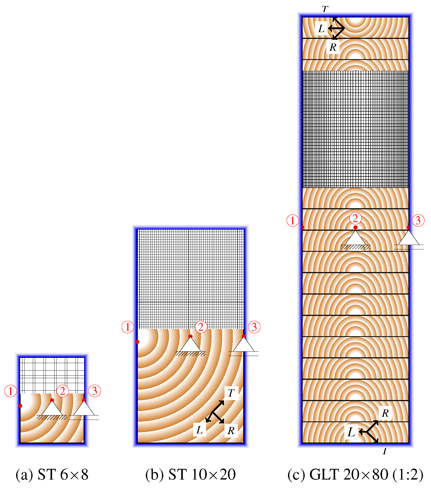
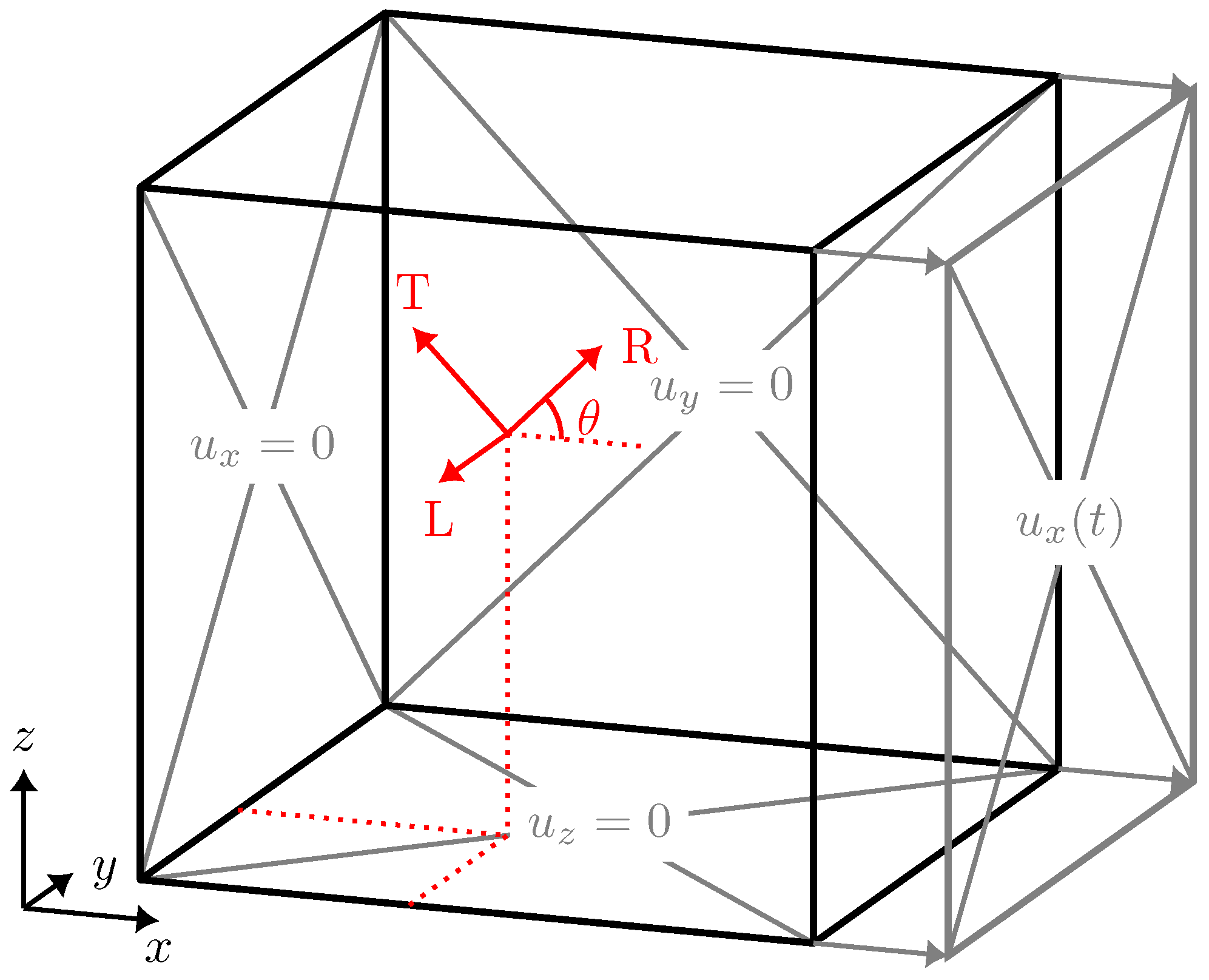
2.3. Geometries, Initial and Boundary Conditions

The long-term influence is investigated using three different rectangular cross-sections with dimensions of 6 × 8 cm and 10 × 20 cm made of solid timber (ST) and 20 × 80 cm made of GLT. The pith, as shown in Figure 1, is located in the center of the left edge for the ST cross-sections and in the axis of symmetry for the GLT cross-section. It defines the center of the cylindrical-orthotropic material coordinate system. The upper lamella of the GLT beam is rotated by 180°. Throughout the hygrothermal analysis, all four edges are exposed to the surrounding climate. The initial conditions correspond to a relative humidity of 65% at 293.15 K, resulting in an MC of 11.73%. The climate conditions over the 14-month period are from Linz, Austria, from 1 November 2014, to 1 January 2016, as given in [23].

The boundary conditions during the mechanical simulation, as depicted in Figure 1, consist of a hinged support in the center of the cross-section and a roller support in the center of the right edge to facilitate free deformation. Given that the cross-section represents a slice of a beam, plane strain conditions were applied in the longitudinal direction.

Figure 1 shows the spatial discretization of the investigated specimens. The finite element meshes consist of 8-node linear brick elements (C3D8). To ensure spatial convergence, a relatively fine mesh with 2542 nodes for the ST 6 × 8, 10,302 nodes for the ST 10 × 20 and 19,642 nodes for GLT 20 × 80 was used.

For an initial study of the model’s prediction capabilities, a single-finite element cube shown in Figure 2, with constant material orientation and an edge length of 20 mm was studied. The setup is similar to the one used in [15], but instead of a load-controlled simulation, a deformation-controlled one is performed.

3. Results and Discussion

The aforementioned material model is applied to various geometries subjected to different load cases. Section 3.1 and Section 3.2 discuss a cube width an edge length of 20 mm and spatially constant material orientation (see Figure 2). The specimen is mechanically deformed and subjected to a hygric loading of five wetting and drying cycles. The same loading is then studied in Section 3.3 using a small ST 6 × 8 cm cross-section. Instead of a uniform MC field, a hygrothermal analysis was performed to determine the non-uniform MC field. Subsequently, in Section 3.4, the cross-sections shown in Figure 1 are analyzed over a 14-month period under real climate conditions.

3.1. Performance of the Mechanical Material Model

The cube specimen was subjected to a radial load ($\theta =0$ in Figure 2) with a constant rate from 0 to 0.025 in 150 h and then unloaded with a constant rate back to 0 over another 150 h. During loading and unloading, five cycles of spatially uniformly distributed wetting to 18% MC and drying to 12% MC were applied. The drying and wetting cycles are observable in Figure 3 in the hygroexpansion strain ${\mathit{\epsilon }}_{\mathrm{RR}}^u$.

All resulting strain components, throughout the investigated time period, are shown in Figure 3. During the first 50 h, the prescribed strain leads to an increase in the elastic and viscoelastic components. Once the stress reaches the yield strength, the elastic strain remains constant and the plastic strain increases. After 62.5 h, the MC increases from the initial level of 12% to 18%, resulting in additional elastic strain and an increase in the irrecoverable mechanosorptive strain, which depends on the highest MC reached so far. The change in MC also induces hygroexpansion and mechanosorption. In the fourth cycle, the stress reaches the yield strength again, leading to a further increase in plastic strain. After the last MC cycle, the prescribed strain continues to increase up to the maximum value, leading to an increase in stress below the yield strength.

During unloading, the prescribed strain decreases. Correspondingly, the elastic and viscoelastic components reduce until another five MC cycles occur. Subsequently, hygroexpansion and mechanosorptive strains vary again. Fracture is not accounted for in this simulation, which leads to the stresses exceeding the tensile strength after about 250 h. The irrecoverable mechanosorptive strains remain constant also during unloading, as the previously highest MC level was not surpassed. In [2], a different approach to determine the irrecoverable mechanosorptive strain was presented, in which the value of the highest MC reached during the analysis was reset after each mechanical loading phase. This method would decrease the component after unloading. The simulation shows that the implemented rheological model behaves as expected during drying and wetting as well as loading and unloading.

3.2. Effect of Uniform Moisture Field Variations

For a detailed study of the influence of a changing MC field on the different components of the rheological model, a cube with a length of 20 mm (as before) was investigated. In this case, the material orientation was rotated by $\theta =45$ degrees (Figure 2) around the longitudinal axis to generate moisture-induced stresses depending on multiple orthotropic expansion coefficients. During the first 150 h, five wetting cycles occur with an increase in MC from 12% to 18%, followed by five drying cycles with a decrease in MC from 12% to 6%. The MC is always uniformly distributed across the sample. To better understand the different components of the rheological model, four different configurations were compared:

• The presented rheological model;
• The presented rheological model without irrecoverable mechanosorption;
• A material model not considering viscoelasticity and mechanosorption and;
• A material model not considering viscoelasticity and mechanosorption, with a constant compliance tensor.

Figure 4 shows the radial stress component for the four different configurations and the mechanosorptive, viscoelastic, and irrecoverable mechanosorptive strains. During an MC cycle, the mechanosorptive strains increase more during the wetting part and decrease less during the drying part, resulting in an overall stepwise increase. The irrecoverable mechanosorptive strains build up in the first cycle as the maximum MC of 18% is reached. During the drying cycles, the mechanosorptive strains decrease after each cycle for opposite reasons as during wetting. This results in opposite signs of the mechanosorptive and irrecoverable mechanosorptive strains and, thus, reduces the overall mechanosorptive effect. A comparison of the material models with constant and MC-dependent stiffness parameters in Figure 4 shows that MC-dependent stiffness values lead to lower stresses during wetting (lower stiffness due to higher MC) than during drying (higher stiffness due to lower MC), as compared to constant stiffness values. This effect leads to larger viscoelastic strains during drying cycles than during wetting cycles. The irrecoverable mechanosorption component that occurs during the first wetting cycle reduces stress values during wetting cycles and enlarges them during drying cycles.

3.3. Effect with Non-Uniform Moisture Field Variations

To investigate the influence of a non-uniform MC field that develops when a wood element is exposed to a realistic climatic condition, the cross-section ST 6 × 8 (Figure 1a) with dimensions 6 by 8 cm was subjected to five wetting and drying cycles. The MC was spatially prescribed using a pre-computed MC field resulting from a multi-Fickian moisture transport model. This transport model accounts for moisture transport phenomena of wood, such as sorption hysteresis. The relative humidity of the ambient air changed in the simulations from an initial 65% to 84% during the wetting and to 26% during the drying cycles. Orthotropic expansion coefficients and a cylindrical coordinate system result in moisture-induced stresses, which are studied at the points shown in Figure 1. To highlight the impact of mechanosorption, creep and plasticity, as well as sorption hysteresis, an additional material model without viscoelasticity and mechanosorption and a model without sorption hysteresis were analyzed.

Figure 5a shows the evolution of the MC at the three points. The points near the boundary (① and ③) respond quickly to changes in the surrounding air, whereas point ② in the center of the cross-section shows very little change. Consideration of sorption hysteresis results in higher MC values at the points near the boundary since the decrease in MC follows a different isotherm that predicts a higher equilibrium MC. Therefore, the increase in the next cycle starts at a higher value, leading to increasing MC values after each cycle. During drying cycles, the decrease of the MC also starts at a higher level and follows the desorption isotherm, again leading to higher MC values. Comparing wetting and drying cycles, the latter shows a higher amplitude in both cases. The effect of hysteresis is also observable in Figure 5b–d, where it leads to smaller changes in stress compared to the simulation results disregarding hysteresis. Again, the amplitudes are smaller during wetting than during drying for both cases.

Comparing the model without viscoelasticity and mechanosorption with the rheological model in Figure 5b, the behavior equals that from Section 3.2: during wetting, the irrecoverable mechanosorptive and mechanosorptive strains have the same sign, i.e., the effects add up. The opposite is true during drying cycles. Throughout the simulation, the absolute viscoelastic strains are smaller than the mechanosorptive ones.

Figure 5c shows the cross-section’s center point values. The cycle’s duration of 15 h is too short for a significant change in MC at the center, thus, viscoelastic strains are dominant. The maximum absolute values of the stresses are also much smaller than those observed at the boundary. However, the stresses in the center of the cross-section are affected by the stresses at the boundary. as can be seen from the changes over time, which are not related to the MC changes, but arise because equilibrium must be reached throughout the cross-section.

Comparing Figure 5b,d, showing results at Points ① and ③ located at opposite sides of the cross-section, the influence of the material orientation becomes evident. As Point ① is close to the pith, for comparison, strains and stresses are shown for the radial direction. Although the MC at the two points is very similar, the resulting strains and stresses differ due to the material orientation-dependent MC expansion coefficients and material stiffness.

Except for the first drying cycle, the absolute values of the stresses from the rheological model in Figure 5b,d are all lower than in the model without viscoelasticity and mechanosorption. The difference is much more pronounced during the wetting cycles than during the drying cycles.

In Figure 6, the stresses resulting from changing the order of drying and wetting cycles (i.e., first drying, then wetting) are shown at the three points within the cross-section. Again, the stress reduction is much more pronounced during the wetting cycles due to the irrecoverable mechanosorptive part. The behavior observed in Figure 5, where drying cycles have larger amplitudes than wetting cycles, is unaffected by the order.

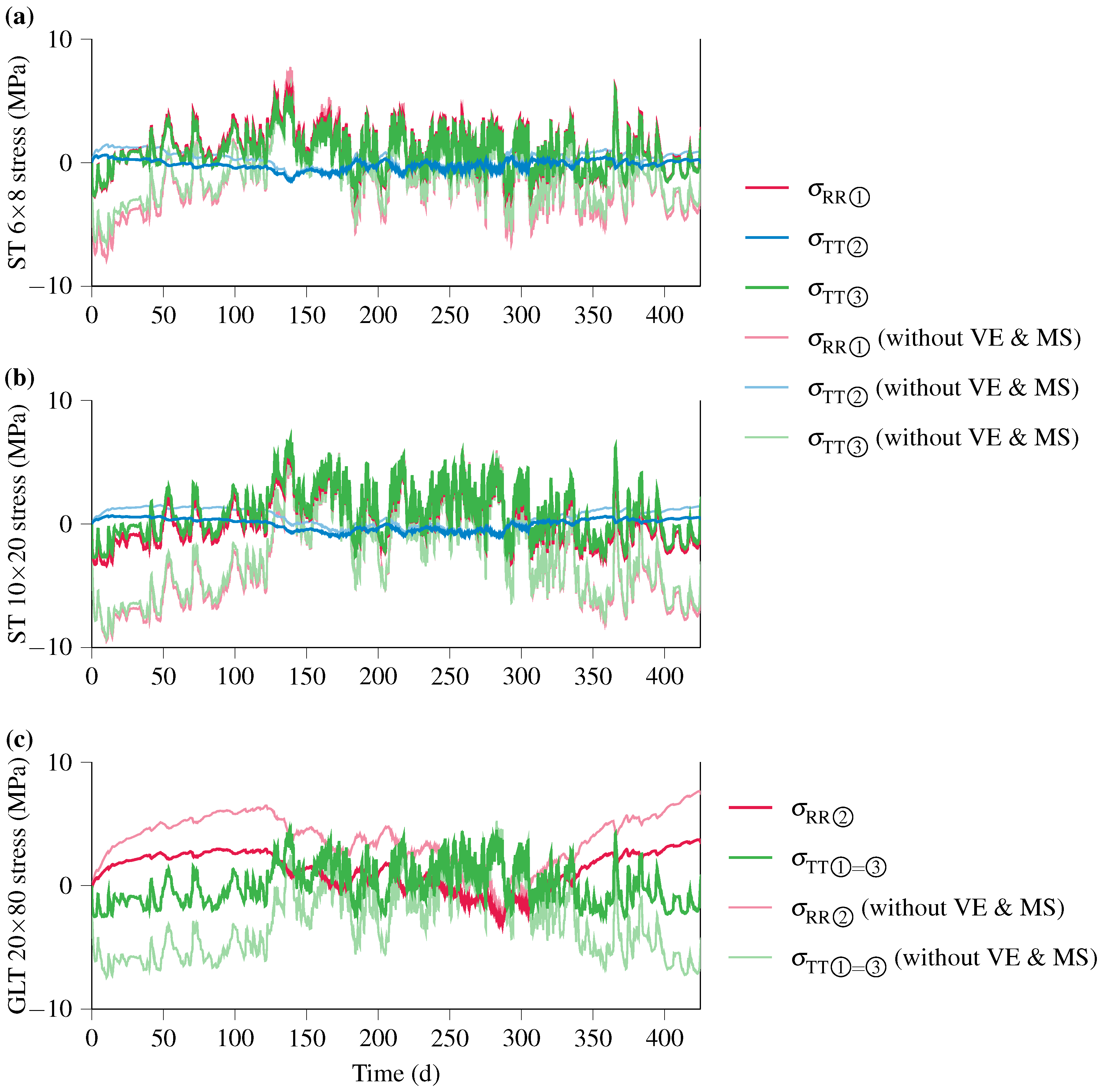
3.4. Effects under Realistic Long-Term Loading

The rheological model is applied to the three cross-sections shown in Figure 1 and analyzed for a 14-month climate of the city of Linz, Austria, between November 2014 and December 2015. First, the MC field, used as loading in the subsequent mechanical analysis step, was computed for the given climate boundary condition.

In Figure 7, the strain components and stress values in the tangential direction at Point ③ are investigated. Figure 7a shows the solution of the presented rheological model in comparison with a material model without viscoelasticity and mechanosorption. The compressive stresses are significantly reduced during the first 120 days, which, roughly, correspond to the months of November to February. This period is referred to as the “wetting period”, because the MC at the boundary is larger than in the center. Thus, the cross-section’s boundary is in compression, whereas the center is in tension. March and the following months until September (day 310) are the “drying period”, during which the MC at the boundary is less than in the center. Thus, tensile stresses dominate at the boundary. These stresses can also reach the tensile strength limit and lead to cracks in the boundary zone. The difference between the two studied material models is significantly smaller during the drying period.

Figure 7b shows the hygroscopic expansion, which is independent of the material model, and the plastic strain. This strain component increases at the beginning of the simulation due to the moist ambient climate, which leads to compressive stresses amounting to the compressive strength, resulting in the accumulation of plastic strains. At the end of the drying period, the plastic strains in Point ③ continue to increase. Figure 7c,d show the viscoelastic and mechanosorptive strains, respectively, resulting from the underlying Kelvin–Voigt elements with different retardation times and moisture contents. The irrecoverable mechanosorption is also shown in Figure 7d. It increases during the wetting periods at the beginning and at the end of the studied time frame.

In Figure 8, all studied cross-sections shown in Figure 1 are compared in terms of stress in the three Points ① to ③ during the 14-month period. The piths of the lamellae of GLT 20 × 80 are located in the symmetry axis. Therefore, in the center, the stress is shown in the radial direction and at the edge in the tangential direction. The behavior during the wetting and drying periods is similar to the previously mentioned examples: the absolute stress decreases more during the wetting period than during the drying period. Thus, the tensile stresses within the cross-section during wetting are smaller when mechanosorption, plasticity, and viscoelasticity are considered.

The significant influence of lower tensile stresses within the cross-section is shown in Figure 9. Each time step was assessed using the crack-prone volume method described in [23]. For a particular time, the crack-prone volume value is the sum of the corresponding volumes of the integration points violating the Tsai–Wu failure criterion presented in [26]. During the wetting period, the crack-prone volume value reaches its maximum value for the simulation without viscoelasticity and mechanosorption. There, as shown exemplarily for the GLT beam, cracks within the cross-section are dominant. In comparison, the rheological model shows far fewer cracks, reflected in an overall very low crack-prone volume.

4. Conclusions

In this work, we presented and applied a material model that combines a multisurface plasticity model [24] with a time-dependent viscoelastic and mechanosorptive material model [6,15], taking into account sorption hysteresis. We investigated the results of the rheological model and simplified material models in various simulations, which led us to the following conclusions:

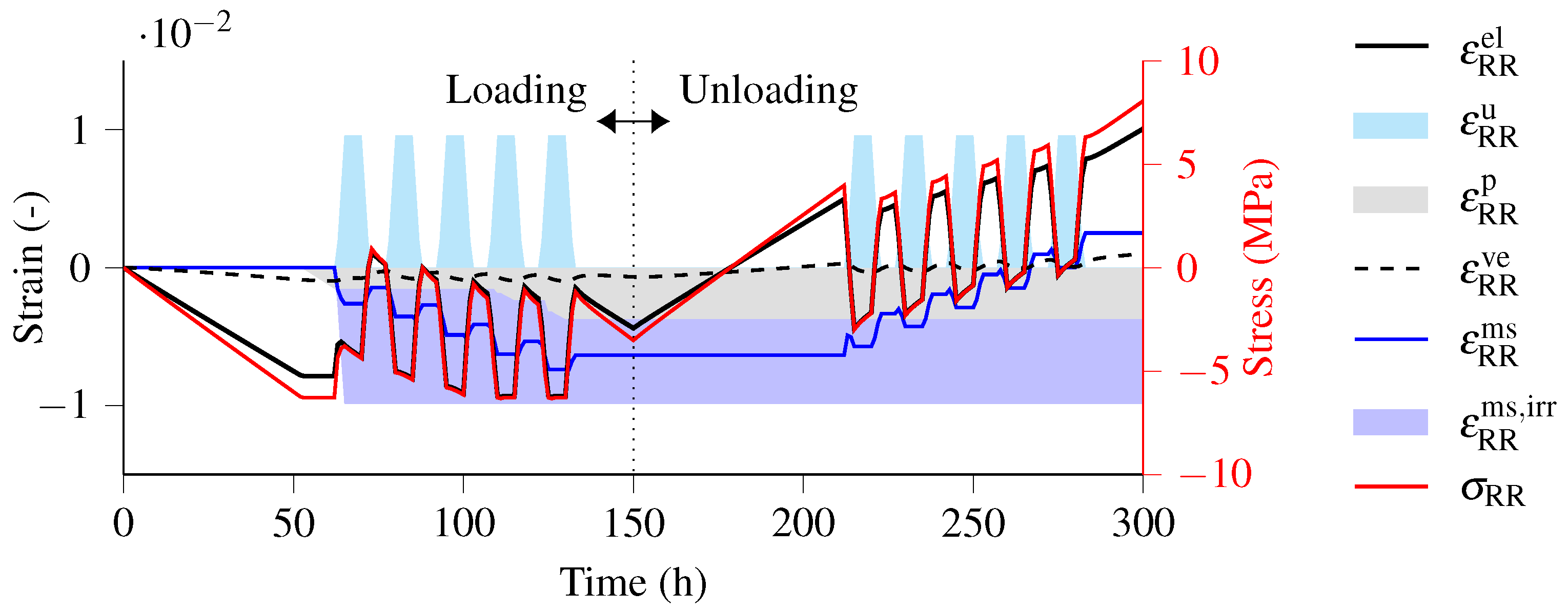
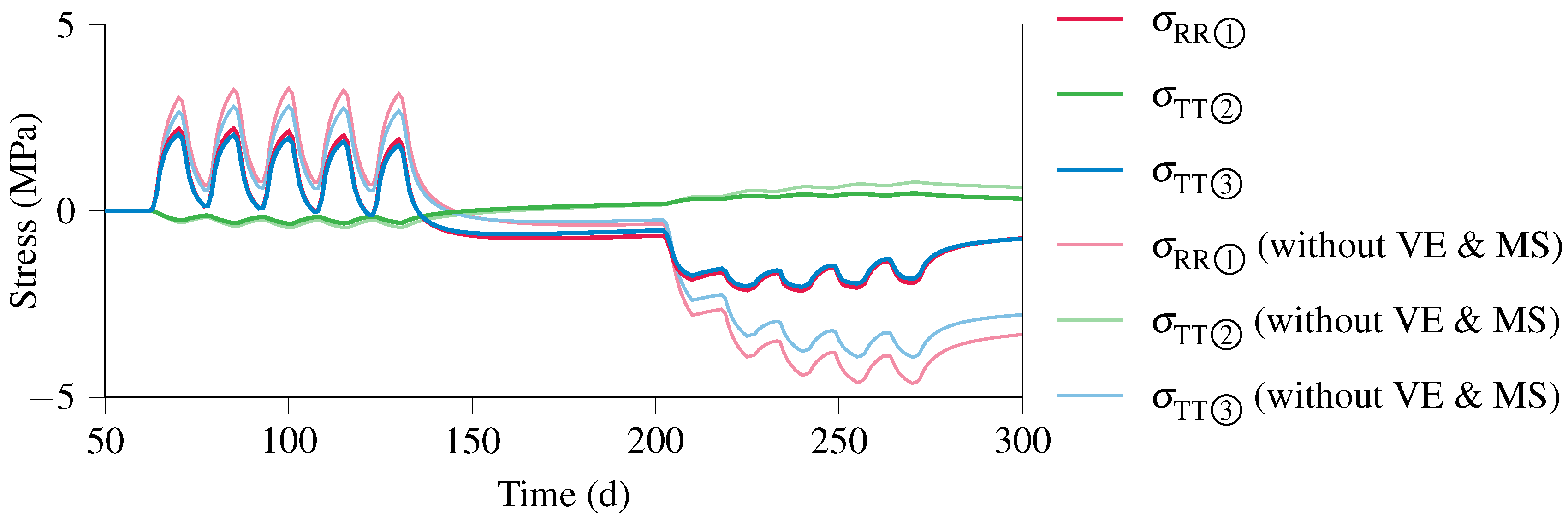
• A moisture-dependent compliance tensor results in smaller absolute stresses during wetting periods and larger absolute stresses during drying periods, as compared to a constant stiffness tensor (Figure 4).
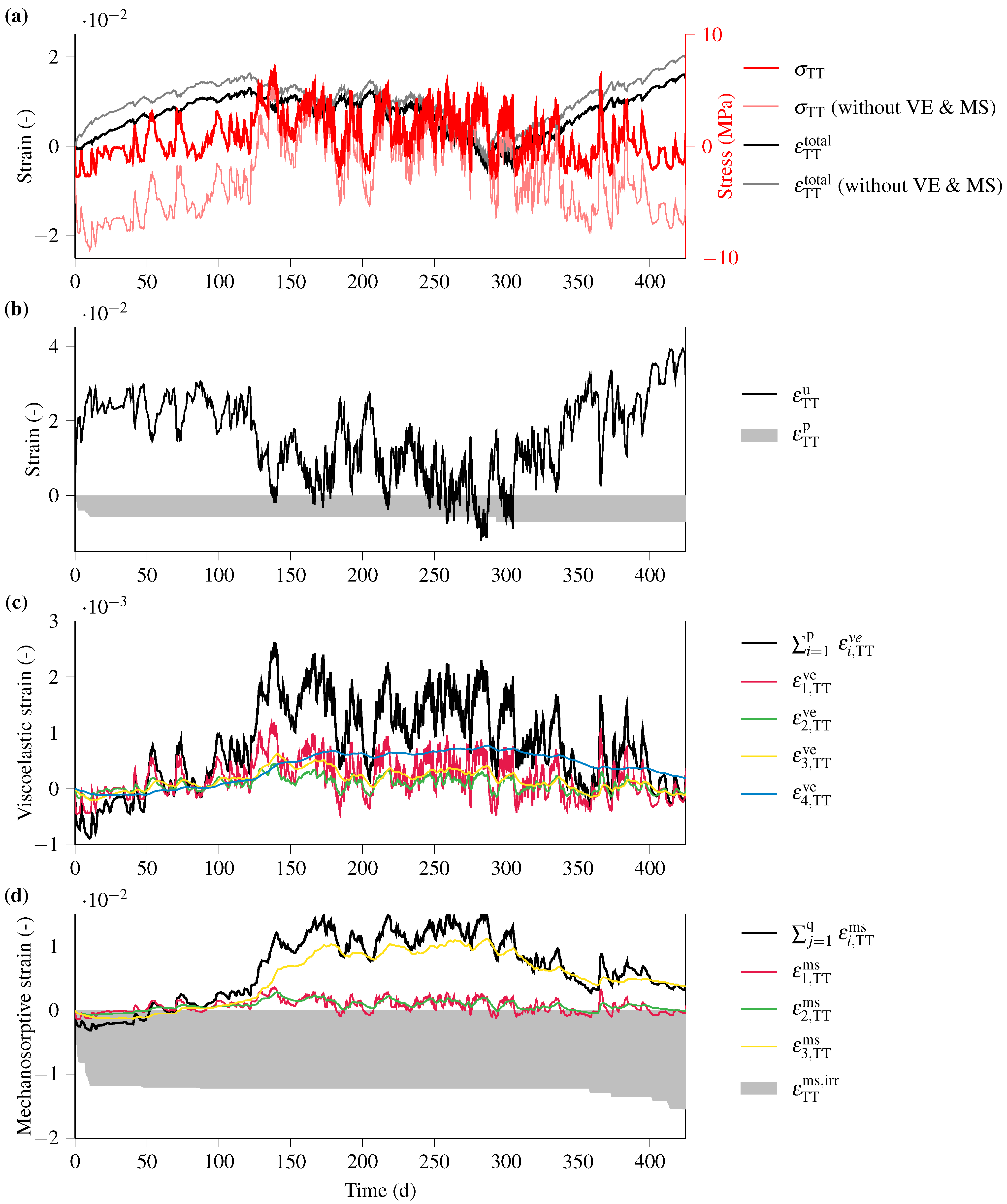
• The irrecoverable part of mechanosorption increases only during wetting periods, which are accompanied by compression, e.g., in the boundary region of the cross-section. During wetting periods, therefore, mechanosorption and irrecoverable mechanosorption add up. However, during drying periods, mechanosorption develops in the opposite direction, up to a value close to the irrecoverable mechanosorption, thus, significantly reducing the total mechanosorptive strains (Figure 5).
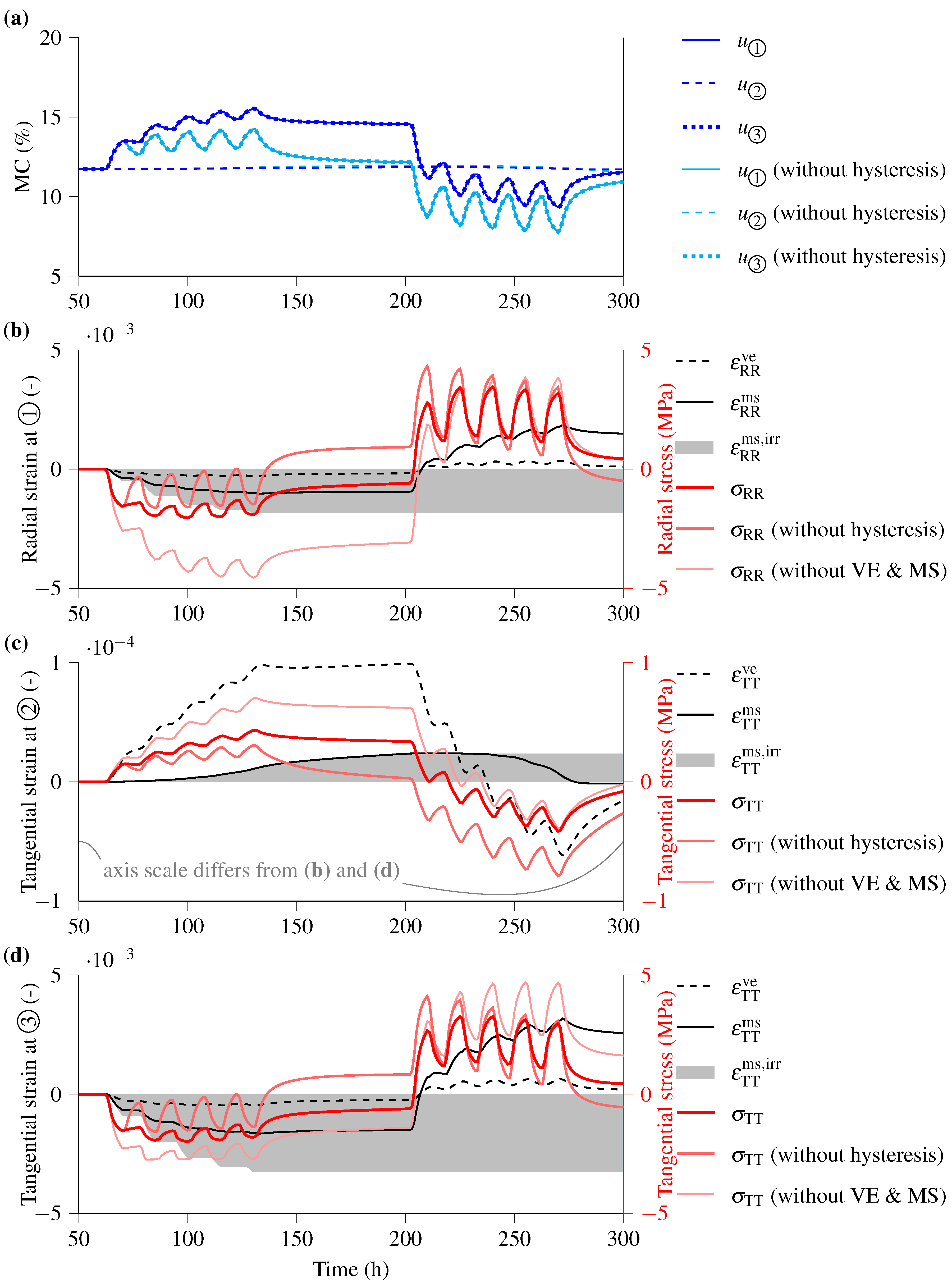
• The consideration of realistic sorption hysteresis affects the moisture content field and, consequently, the stresses under changing climatic conditions. This leads to a step-wise increase in moisture content under cyclic humidity changes, thus resulting in larger moisture-induced loading (Figure 5).
• During a 14-month climatic cycle, the resulting stresses were found to be significantly more affected during the wetting period (with moisture content being greater at the edge than in the center) than during the drying period.
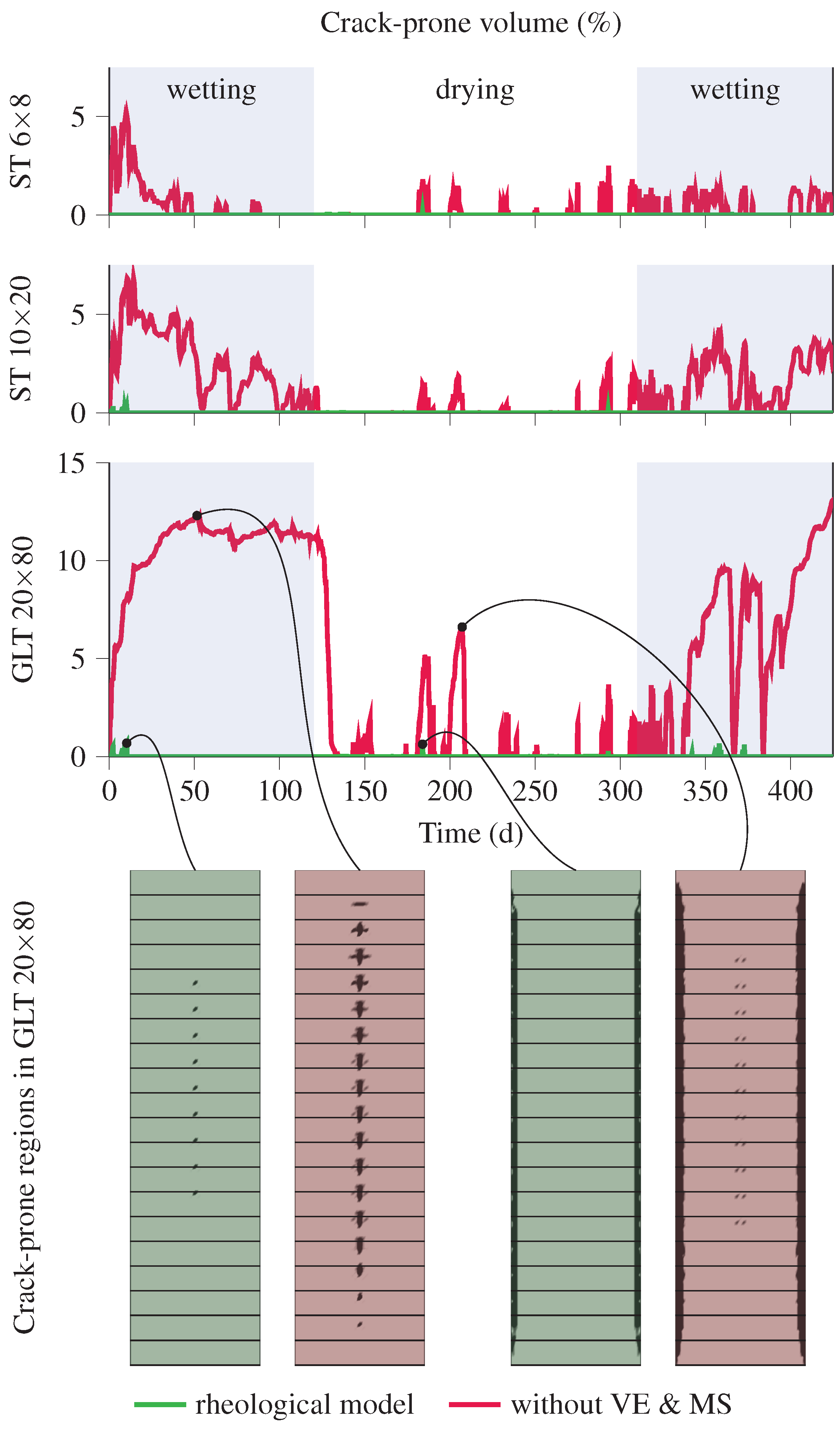
• During the wetting period, stress relaxation at the edge of the cross-section reduces the stress levels in the center of the cross-section, bringing them below the threshold where cracks could potentially form. This finding validates the empirical understanding that cracks are more likely to occur on the surface under drying conditions, rather than inside a cross-section due to wetting.

In conclusion, it can be stated that crack predictions based on models not accounting for viscoelasticity and mechanosorption are conservative, but under dry conditions, they offer valuable insights for engineering comprehension [34]. Conversely, in cases of wetting conditions, it is essential to consider time-dependent and moisture-dependent material effects to attain realistic stress levels.

References

1. Dietsch, P.; Gamper, A.; Merk, M.; Winter, S. Monitoring Building Climate and Timber Moisture Gradient in Large-Span Timber Structures. J. Civil Struct. Health Monit. 2015, 5, 153–165. [Google Scholar] [CrossRef]
2. Yu, T.; Khaloian, A.; van de Kuilen, J.W. An improved model for the time-dependent material response of wood under mechanical loading and varying humidity conditions. Eng. Struct. 2022, 259, 114116. [Google Scholar] [CrossRef]
3. Hanhijärvi, A.; Mackenzie-Helnwein, P. Computational Analysis of Quality Reduction during Drying of Lumber due to Irrecoverable Deformation. I: Orthotropic Viscoelastic-Mechanosorptive-Plastic Material Model for the Transverse Plane of Wood. J. Eng. Mech. 2003, 129, 996–1005. [Google Scholar] [CrossRef]
4. Toratti, T.; Svensson, S. Mechano-sorptive experiments perpendicular to grain under tensile and compressive loads. Wood Sci. Technol. 2000, 34, 317–326. [Google Scholar] [CrossRef]
5. Svensson, S.; Toratti, T. Mechanical response of wood perpendicular to grain when subjected to changes of humidity. Wood Sci. Technol. 2002, 36, 145–156. [Google Scholar] [CrossRef]
6. Fortino, S.; Mirianon, F.; Toratti, T. A 3D moisture-stress FEM analysis for time dependent problems in timber structures. Mech. Time-Depend. Mater. 2009, 13, 333. [Google Scholar] [CrossRef]
7. Reichel, S.; Kaliske, M. Hygro-mechanically coupled modelling of creep in wooden structures, Part I: Mechanics. Int. J. Solids Struct. 2015, 77, 28–44. [Google Scholar] [CrossRef]
8. Santaoja, K.; Leino, T.; Ranta-Maunus, A.; Hanhijärvi, A. Mechano-Sorptive Structural Analysis of Wood by the ABAQUS Finite Element Program; Number 1276 in Valtion Teknillinen Tutkimuskeskus; Tiedotteita, VTT Technical Research Centre of Finland: Espoo, Finland, 1991. [Google Scholar] [CrossRef]
9. Ranta-Maunus, A. Impact of mechano-sorptive creep to the long-term strength of timber. Holz Roh Werkst. 1990, 48, 67–71. [Google Scholar] [CrossRef]
10. Leicester, R.H. A Rheological Model for Mechano-Sorptive Deflections of Beams. Wood Sci. Technol. 1971, 5, 211–220. [Google Scholar] [CrossRef]
11. Salin, J.G. Numerical Prediction of Checking during Timber Drying and a New Mechano-Sorptive Creep Model. Holz Roh-und Werkst. 1992, 50, 195–200. [Google Scholar] [CrossRef]
12. Mackenzie-Helnwein, P.; Hanhijärvi, A. Computational Analysis of Quality Reduction during Drying of Lumber due to Irrecoverable Deformation. II: Algorithmic Aspects and Practical Application. J. Eng. Mech. 2003, 129, 1006–1016. [Google Scholar] [CrossRef]
13. Reichel, S.; Kaliske, M. Hygro-mechanically coupled modelling of creep in wooden structures, Part II: Influence of moisture content. Int. J. Solids Struct. 2015, 77, 45–64. [Google Scholar] [CrossRef]
14. Fortino, S.; Hradil, P.; Metelli, G. Moisture-induced stresses in large glulam beams. Case study: Vihantasalmi Bridge. Wood Mater. Sci. Eng. 2019, 14, 366–380. [Google Scholar] [CrossRef]
15. Hassani, M.M.; Wittel, F.K.; Hering, S.; Herrmann, H.J. Rheological model for wood. Comput. Methods Appl. Mech. Eng. 2015, 283, 1032–1060. [Google Scholar] [CrossRef]
16. Frandsen, H.L. Selected Constitutive Models for Simulating the Hygromechanical Response of Wood. Ph.D. Thesis, Aalborg University, Aalborg, Denmark, 2007. [Google Scholar]
17. Schniewind, A.P.; Barrett, J.D. Wood as a Linear Orthotropic Viscoelastic Material. Wood Sci. Technol. 1972, 6, 43–57. [Google Scholar] [CrossRef]
18. Huč, S.; Svensson, S. Influence of Grain Direction on the Time-Dependent Behavior of Wood Analyzed by a 3D Rheological Model. A Mathematical Consideration. Holzforschung 2018, 72, 889–897. [Google Scholar] [CrossRef]
19. Huč, S.; Svensson, S.; Hozjan, T. Hygro-Mechanical Analysis of Wood Subjected to Constant Mechanical Load and Varying Relative Humidity. Holzforschung 2018, 72, 863–870. [Google Scholar] [CrossRef]
20. Huč, S.; Svensson, S.; Hozjan, T. Numerical Analysis of Moisture-Induced Strains and Stresses in Glued-Laminated Timber. Holzforschung 2020, 74, 445–457. [Google Scholar] [CrossRef]
21. Autengruber, M.; Lukacevic, M.; Gröstlinger, C.; Eberhardsteiner, J.; Füssl, J. Numerical assessment of wood moisture content-based assignments to service classes in EC5 and a prediction concept for moisture-induced stresses solely using relative humidity data. Eng. Struct. 2021, 245, 112849. [Google Scholar] [CrossRef]
22. Autengruber, M.; Lukacevic, M.; Füssl, J. Finite-element-based moisture transport model for wood including free water above the fiber saturation point. Int. J. Heat Mass Tran. 2020, 161, 120228. [Google Scholar] [CrossRef]
23. Autengruber, M.; Lukacevic, M.; Gröstlinger, C.; Füssl, J. Finite-element-based prediction of moisture-induced crack patterns for cross sections of solid wood and glued laminated timber exposed to a realistic climate condition. Constr. Build. Mater. 2021, 271, 121775. [Google Scholar] [CrossRef]
24. Pech, S.; Lukacevic, M.; Füssl, J. A robust multisurface return-mapping algorithm and its implementation in Abaqus. Finite Elem. Anal. Des. 2021, 190, 103531. [Google Scholar] [CrossRef]
25. Lukacevic, M.; Füssl, J.; Lampert, R. Failure mechanisms of clear wood identified at wood cell level by an approach based on the extended finite element method. Eng. Fract. Mech. 2015, 144, 158–175. [Google Scholar] [CrossRef]
26. Lukacevic, M.; Lederer, W.; Füssl, J. A microstructure-based multisurface failure criterion for the description of brittle and ductile failure mechanisms of clear-wood. Eng. Fract. Mech. 2017, 176, 83–99. [Google Scholar] [CrossRef]
27. Krabbenhøft, K.; Damkilde, L. A model for non-Fickian moisture transfer in wood. Mater. Struct. 2004, 37, 615–622. [Google Scholar] [CrossRef]
28. Frandsen, H.L.; Damkilde, L.; Svensson, S. A revised multi-Fickian moisture transport model to describe non-Fickian effects in wood. Holzforschung 2007, 61, 563–572. [Google Scholar] [CrossRef]
29. Frandsen, H.L.; Damkilde, L.; Svensson, S. A hysteresis model suitable for numerical simulation of moisture content in wood. Holzforschung 2007, 61, 175–181. [Google Scholar] [CrossRef]
30. Frandsen, H.L.; Damkilde, L.; Svensson, S. Implementation of sorption hysteresis in multi-Fickian moisture transport. Holzforschung 2007, 61, 693–701. [Google Scholar] [CrossRef]
31. O’Ceallaigh, C.; Sikora, K.; McPolin, D.; Harte, A.M. Modelling the hygro-mechanical creep behaviour of FRP reinforced timber elements. Constr. Build. Mater. 2020, 259, 119899. [Google Scholar] [CrossRef]
32. Tsai, S.W.; Wu, E.M. A General Theory of Strength for Anisotropic Materials. J. Compos. Mater. 1971, 5, 58–80. [Google Scholar] [CrossRef]
33. Simo, J.C.; Hughes, T.J. Computational Inelasticity; Springer Science & Business Media: Berlin/Heidelberg, Germany, 1998; Volume 7. [Google Scholar] [CrossRef]
34. Brandstätter, F.; Autengruber, M.; Lukacevic, M.; Füssl, J. Prediction of Moisture-Induced Cracks in Wooden Cross Sections Using Finite Element Simulations. Wood Sci. Technol. 2023, 57, 671–701. [Google Scholar] [CrossRef] [PubMed]
Figure 1. Investigated cross-sections ST 6 × 8, ST 10 × 20 and GLT 20 × 80, with the used finite element mesh (the reader is referred to the online version of this article for a more precise visualization of the element edges). Result values are evaluated at Points ① to ③, marked in red. The blue boundary depicts the location of the boundary conditions during the hygrothermal analysis, and the supports show the type and location of the boundary conditions during the mechanical analysis. The material orientation is shown for each cross-section individually. The size of the GLT 20 × 80 is scaled by 0.5 compared to the other cross-sections.
Buildings 14 00937 g001
Figure 2. Boundary conditions and local material coordinate system for the investigated cube with an edge length of 20 mm.
Buildings 14 00937 g002
Figure 3. Resulting radial elastic (el), hygroexpansion (u), plastic (p), viscoelastic (ve), meachnosorptive (ms), and irrecoverable meachnosorptive (ms,irr) strain components and radial stress when a cube with a length of 20 mm is subjected to a predefined strain in the radial direction. Five wetting cycles take place during loading (0–150 h) and unloading (150–300 h).
Buildings 14 00937 g003
Figure 4. Viscoelastic (ve), mechanosorptive (ms), and irrecoverable mechanosorptive (ms,irr) strains (black) during five wetting followed by five drying cycles in radial direction as well as stresses (red) evaluated for four material models.
Buildings 14 00937 g004
Figure 5. (a) MC and (bd) strains (black) and stresses (red) during five wetting followed by five drying cycles, evaluated at three points of the cross-section shown in Figure 1a. Stresses are shown for models with and without mechanosorption, creep, and plasticity, as well as without sorption hysteresis.
Buildings 14 00937 g005
Figure 6. Comparison of stresses during five drying followed by five wetting cycles at three points of the cross-section shown in Figure 1a. Stresses of the rheological model and the linear model without viscoelasticity and mechanosorption are shown.
Buildings 14 00937 g006
Figure 7. Additively combined strains and stresses for the cross-section ST 10 × 20 at Point ③ (Figure 1) in tangential direction. (a) shows the stresses, and total strains of a material model with and without viscoelasticity and mechanosorption. (bd) show the individual values of the strain components part of the rheological model from Equation (1).
Buildings 14 00937 g007
Figure 8. Stresses of cross-sections ST 6 × 8 (a), ST 10 × 20 (b) and GLT 20 × 80 (c) (shown in Figure 1) at Points ① to ③, evaluated with the presented rheological model and a model without viscoelasticity and mechanosorption.
Buildings 14 00937 g008
Figure 9. Assessment of the crack-prone volume when taking into account the presented rheological model. Damaged areas withing the cross-section are visualized for the GLT 20 × 80. The amount of crack-prone volume can be heavily reduced by considering a comprehensive rheological model.
Buildings 14 00937 g009
Disclaimer/Publisher’s Note: The statements, opinions and data contained in all publications are solely those of the individual author(s) and contributor(s) and not of MDPI and/or the editor(s). MDPI and/or the editor(s) disclaim responsibility for any injury to people or property resulting from any ideas, methods, instructions or products referred to in the content.