
A Machine Learning Model to Predict the Seismic Lifecycle Behavior of a Cross-Sea Cable-Stayed Bridge

School of Civil Engineering and Architecture, Hainan University, Haikou 570228, China
*
Author to whom correspondence should be addressed.
Buildings 2024, 14(5), 1190; https://doi.org/10.3390/buildings14051190
Submission received: 3 April 2024
/
Revised: 18 April 2024
/
Accepted: 20 April 2024
/
Published: 23 April 2024
(This article belongs to the Topic New Trends in Advanced Construction Technology, Sustainable Construction Materials and High-Performance Building Structures)
Abstract
:Cross-sea cable-stayed bridges encounter challenges associated with cable corrosion and cable-force relaxation during their service life, which significantly affects their structural performance and seismic response. This study focuses on a cross-sea cable-stayed bridge located in Hainan Province. Utilizing an LSTM deep learning model, this study aims to fill in the gaps in short-term cable-monitoring data from the past year using the available cable-force-monitoring data from the same period. The authors of this study interpolated the cable-force data in the absence of sensors and employed a SARIMA machine learning time-series-prediction model to predict the future trends of all cable forces. A finite-element model was constructed, and a dynamic time-history analysis of the seismic response of the cross-sea cable-stayed bridge was conducted, considering the influence of cable-force relaxation and cable corrosion in the future. The findings indicate that the LSTM-SARIMA model predicted an average decrease of 11.81% in the cable force of the cable-stayed bridge after 20 years. During the lifecycle of the cables, cable corrosion exerts a significant impact on the variation in cable stress within the bridge structure during earthquakes, while cable-force relaxation has a more pronounced effect on the vertical displacement of the main beam of the bridge structure during seismic events. Compared to when using the traditional model that only considers cable corrosion, the maximum negative vertical displacement of the main beam increases by 29.7% when using the proposed model if the earthquake intensity is 0.35 g after 20 years, which indicates that the proposed machine learning model can exactly determine the seismic behavior of the lifecycle cross-sea cable-stayed bridge, considering the impacts of both cable-force relaxation and cable corrosion.
1. Introduction
Cable-stayed bridges have emerged as the primary bridge type for long-span structures due to their elegant design and remarkable load-bearing capacity. Currently, cable-stayed bridges often face issues such as corrosion, cable tension relaxation, and seismic events, which pose threats to their safety. In contemporary research, the combined effects of cable corrosion and tension relaxation under seismic conditions throughout the lifecycle of the cables are generally not considered. Given that many bridges are equipped with sensors that have gathered extensive data on cable tensions, it is feasible to employ machine learning models to predict cable tensions. In cable-stayed bridges, monitoring the cable force is essential to ensure their safe operation and promptly detect any risks. However, due to cost or technological constraints, many cable-stayed bridges do not implement full cable monitoring, often equipping only a portion of the cables with force sensors [1]. Additionally, monitoring processes frequently encounter missing or abnormal values [2]. As a result, the cable-force-monitoring data on the entire bridge are typically incomplete, necessitating the supplementation of corresponding cable forces.
Machine learning is a method that enables computer systems to automatically improve and optimize performance by learning patterns and rules from data. It focuses on discovering patterns, making predictions, or making decisions based on data by constructing and training models. Driven by advancements in computer and artificial intelligence technologies, machine learning is increasingly applied in civil engineering. Zain et al. [3,4] proposed a novel framework for assessing the vulnerability of tubular structures using machine learning algorithms and investigated the effectiveness of using vulnerability information for tubular buildings through machine learning. Xu et al. [5] assessed the seismic damage to reinforced concrete structures using computer vision and machine learning. Asgarkhani et al. [6] applied machine learning to the prediction of residual drift and seismic risk in moment-resisting frames considering soil–structure interactions. Kazemi et al. [7] applied machine learning to assess the seismic fragility and seismic vulnerability of reinforced concrete structures. Ye et al. [8] utilized machine learning to predict and issue early warnings for wind-induced vibrations in cable-stayed bridge towers.
Deep learning, a special form of machine learning, mimics the structure and function of the human neural system and employs artificial neural networks to learn and make decisions. The long short-term memory (LSTM) network, introduced by Hochreiter [9], is a unique type of recurrent neural network proficient at efficiently processing and retaining long-term dependency information within sequence data. LSTM is extensively applied in bridge-health monitoring. For instance, Xu et al. [10] utilized LSTM to predict the time history of nonlinear structures under seismic excitation, with a confidence level within the ±5% interval at 90.2%. Additionally, Liu et al. [11] employed the BP-LSTM hybrid model to evaluate and predict the spatial temperature field and temperature effect of a steel–concrete composite bridge deck system in real-time. Finally, Liu et al. [12] utilized the LSTM model to predict missing data in the temperature monitoring of the Nanjing Dashengguan Yangtze River bridge structure. At the highest prediction accuracy, the mean squared error value was only 0.36.
The seasonal autoregressive integrated moving average (SARIMA) is a widely utilized machine learning time-series-prediction model designed for handling data that exhibit seasonal patterns. It serves as an extension of the ARIMA model, enabling the capture of seasonal variations in data and providing more accurate predictions for time series data with seasonal patterns. SARIMA is recognized as a powerful tool for processing time series data. Cheng et al. [13] employed the SARIMA time-series-forecasting model to forecast the price trends of Bitcoin. Agyemang et al. [14] utilized the SARIMA time-series forecasting model to predict the occurrence of road traffic accidents. Cui et al. [15] applied the SARIMA time-series-forecasting model to the prediction of carbon emissions. In the domain of bridge-health monitoring, Chen et al. [2] employed the SARIMA model to forecast the changes in acceleration values at certain monitoring points on a bridge, and the MAE value was only 0.013. Ping [16] utilized the SARIMA model to forecast and impute missing values for the internal temperature of the main beam in bridge-monitoring data, and the MAE value was only 0.102. Thus, it is evident that the SARIMA model is highly precise in data forecasting during the operation and maintenance of bridges.
For bridges lacking full cable monitoring of the stay cables, the absence of monitoring data for unmonitored stay cables presents a challenge. Therefore, investigating the spatial correlation of stay-cable-force data and predicting the force data on unmonitored stay cables is necessary. Yin et al. [17] discovered in their research on the spatial correlation among groups of stay cables that neighboring stay cables exhibited a high degree of spatial correlation. Additionally, the stay cables with high spatial correlation demonstrated a high level of consistency in terms of cable-force trends and fluctuation magnitudes. Zeng [18] utilized an initialization method based on the improved grey relational analysis theory to study the spatial correlation of stay cables. Correlation data were obtained through the method of cable-break analysis.
Following the completion and opening of cable-stayed bridges, the bearing capacity of stay cables diminishes due to the influence of roadway loads and various environmental factors [19,20,21]. Corrosion, in particular, poses a significant threat to stay cables, leading to a decrease in their seismic resistance. The reduction in the strength of these wires, primarily caused by corrosion, is the primary reason for the decrease in the strength of stay cables [22]. Fuente [23] conducted experiments to investigate the corrosion rate of low-carbon steel under different environmental conditions. Taking into account the influences of environmental temperature, relative humidity, and chloride-ion-corrosion concentration, Klinesmith et al. [24] developed a corrosion-rate-calculation model for stay-cable steel wires. Building on the formula proposed by Klinesmith, Lu and He [25] considered the impact of steel-wire stress on the corrosion of stay cables and proposed a calculation model for the corrosion amount of stay-cable steel wires, taking stress into account.
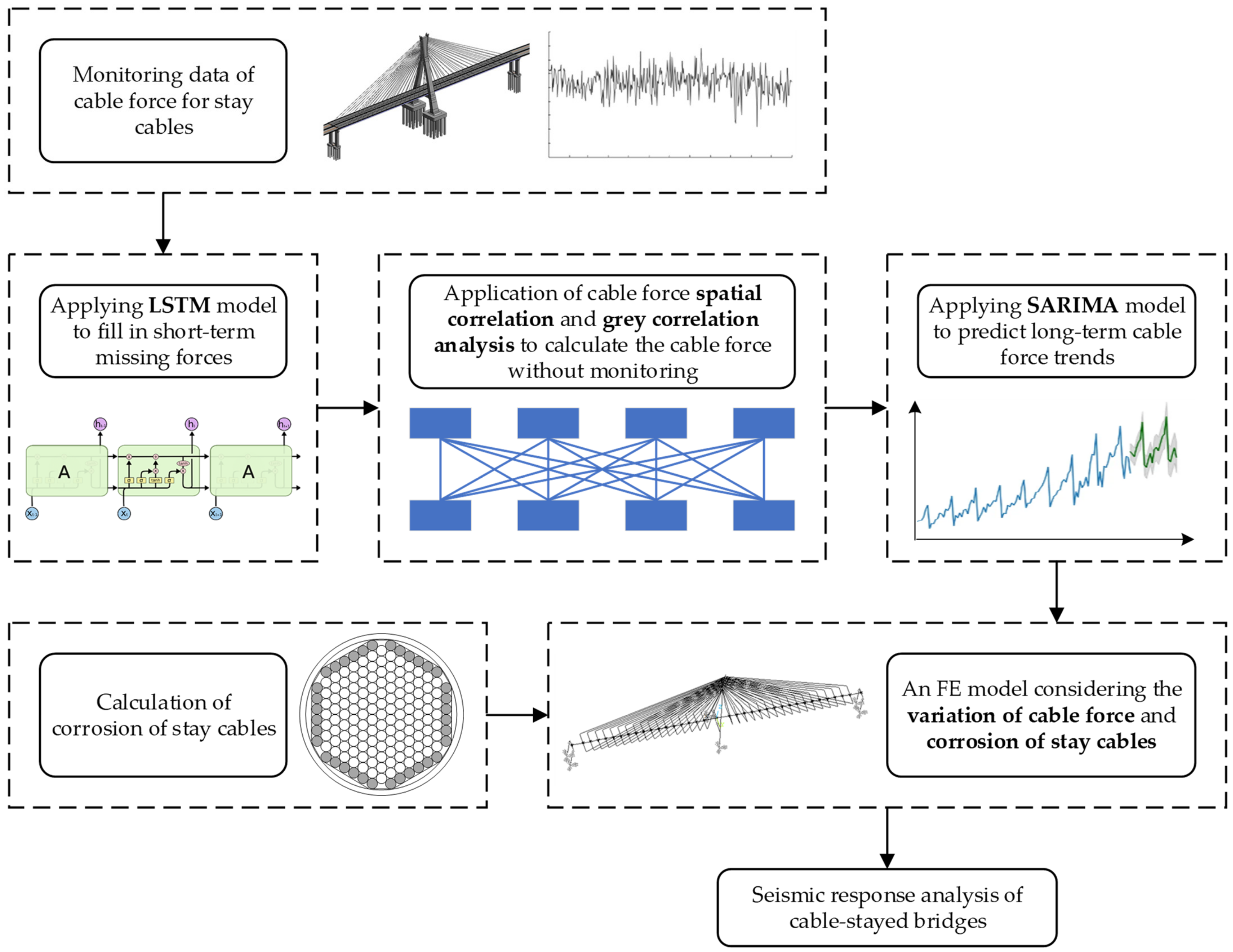
The authors of this study employed the LSTM model, which can effectively capture data patterns, to fill in the missing data of stay cables, and subsequently utilized the spatial correlation of stay-cable forces to gather comprehensive data on the forces exerted by all stay cables. The SARIMA model, which can better reflect the data periodicity and trends, was then utilized to predict the trend of long-term cable-force data, enabling the future state of cable force to be determined. Based on existing research findings and experimental data, the corrosion condition of the stay cables was calculated to determine their future corrosion status. Finally, considering the long-term variation in the cable force and corrosion of stay cables, a long-term seismic-response analysis of a cable-stayed bridge was conducted using the finite-element (FE) method. The application process is illustrated in Figure 1. The innovative work presented in this paper is manifested in the following aspects: (1) The introduction of an LSTM-SARIMA forecasting model for the long-term trend of cable forces in cable-stayed bridges. Compared to conventional calculations, this model incorporates the impacts of various external loads such as wind load and lane load on cable tension. It allows for predictions to be directly made from existing cable-force-monitoring data, thereby enhancing the accuracy of cable-force forecasts. (2) In current seismic analyses of the lifecycles of cable-stayed bridges, traditional methods generally do not consider the combined effects of cable relaxation and corrosion. This study considers both factors simultaneously, making the seismic response more consistent with actual working conditions.
2. Methods
2.1. FE Model of Cross-Sea Cable-Stayed Bridge
The main bridge of the cable-stayed bridge is a single-tower, double-plane, steel box beam cable-stayed bridge, with the stay cables arranged in a fan pattern, utilizing 1670 MPa parallel steel wire stay cables; the stay-cable sheaths are made of PE, and the wires are composed of galvanized steel wire with a 7 mm diameter. The main tower part has an “A”-shaped structure, and the main beam is constructed using a steel box girder. A schematic diagram of the cable-stayed bridge is shown in Figure 2a, and the sheathing of the stay cable and the steel wires are as illustrated in Figure 2b. This cable-stayed bridge is located in Haikou, Hainan Province, China, situated in a tropical marine and humid environment, and is subjected to severe corrosion threats. Moreover, this cable-stayed bridge is located in the Dongzhai Port-Qinglan Port fault zone, where the probability of seismic activity is high. Therefore, this cable-stayed bridge has high research value. This bridge is equipped with cable-force sensors on selected stays, providing a foundational dataset for subsequent research.
The FE model of the cable-stayed bridge was created using ANSYS 2022R2 APDL [26] software. To reduce the computational load of the model, the model’s solid elements were simplified into beam elements, link elements, combined elements, etc., with the main bridge employing a simplified modeling approach based on a spine-beam-calculation model. The definition of a simplified element is as described in Table 1.
The cross-section of the steel box beam is shown in Figure 3. Its cross-sectional area is 2.024 m2, and the moments of inertia are Iyy = 3.420 m4 and Izz = 231.624 m4.
The bridge piers and the bottom of the main tower are fully constrained. The constraints of the main beam, main tower, and auxiliary pier are shown in Table 2.
The method for defining the initial strain of the cable Link10 element was used to apply the cable force. The initial strain was calculated using the cable force, cross-sectional area, elastic modulus, etc. For specific details regarding FE modeling, one may refer to reference [27]. The FE model of the main bridge of the constructed cable-stayed bridge is depicted in Figure 4.
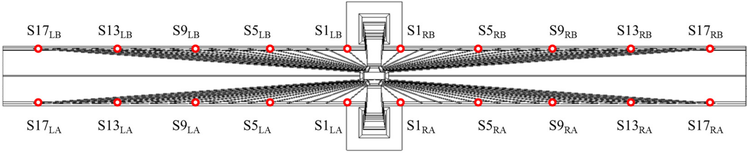
The cable-force sensors of the cable-stayed bridge are arranged on the cables at S1, S5, S9, S13, and S17, as shown in Figure 5. Angle markers L, R, A, and B are used to distinguish the cables in different areas.
2.2. LSTM Model for Short-Term Cable Monitoring
2.2.1. Data Preprocessing of LSTM Model
In LSTM networks, the propagation of gradients is expanded over time, and long-sequence data may cause gradients to gradually disappear or explode in the process of back propagation. By normalizing the input data to an appropriate range, these problems can be alleviated, making the gradient propagation more stable and helping to improve the training efficiency and performance of the model. At the same time, normalization processing can reduce the complexity of the data and reduce the sensitivity of the model to noise and outliers, to improve the generalization ability of the model to unknown data.
Common normalization methods include min–max normalization and standard score normalization. Standard score normalization is a technique that scales data attributes to have a zero mean and unit variance. This method is suitable for cases where the attributes follow a normal distribution. Standard score normalization is conducted according to Formula (1):
where x = the original data point; μ = the average value of the data; and σ = the standard deviation of the data.
The Shapiro–Wilk test is a statistical method used to test whether a sample comes from a normal distribution. This test is predicated on the discrepancies between the observed values of the sample and the expected values under normal distribution. The null hypothesis of the Shapiro–Wilk test posits that the sample is derived from a normal distribution. Should the p-value be less than the significance level (commonly set at 0.05), sufficient evidence exists to reject the null hypothesis, thereby disputing the assumption that the sample is from a normal distribution. The statistic is computed in accordance with Formula (2).
where x(i) = the ordered sample values; = the sample mean; and ai = specific coefficients based on the sample size and the normal distribution. The p-value represents the probability of observing the test statistic W as being as extreme as, or more extreme than, the actual observed values, under the assumption that the null hypothesis is true.
2.2.2. Application of LSTM Model in Short-Term Cable Monitoring
A short-term prediction model of stay-cable force based on the LSTM algorithm was realized by compiling a Python program. After the data were tested for normal distribution using the Shapiro–Wilk test, they were normalized and brought into the model for learning and prediction. The output results were de-normalized and restored to the order of magnitude of the original data.
One of the cable-force test datasets for a period of time was selected as the sample data, taking the first 70% as the training set and the last 30% as the test set, and the accuracy of the model prediction was evaluated. As shown in Figure 6, the predicted and actual values fit well. The average error between the predicted values calculated by the LSTM model and the original values measured by sensors is 0.16%.
2.3. Grey Relation Analysis for Cable-Force Spatial Correlation
2.3.1. Grey Relation Analysis Theory
Grey relational analysis (GRA) is a multifactor statistical analysis method employed to examine the relative intensity of influence exerted by various factors on a particular item of interest within a grey system. It measures the magnitude of association among factors by calculating the grey relational degree among them, which clarifies which factors have a greater impact on the system and which have lesser. This method facilitates the ranking and analysis of factors within complex systems, thereby enhancing their understanding and optimization.
In grey relational analysis, commonly employed data-standardization methods include mean normalization, normalization, interval scaling, and initial-value processing, among others. These techniques are integral for preparing the data for analysis, ensuring comparability and consistency across different scales and dimensions. Formulas (3) and (4) represent the calculation formulas for the mean normalization process; ξ = 0.5 is typically assumed.
2.3.2. The Application of Grey Relational Analysis in Determining the Cable-Force Spatial Correlation
Based on the previous studies by Yin and Zeng et al. [17,18], considering the disconnection of each stay cable, the average change rate of other cable forces was calculated, which is used as the critical index to discriminate the strength of spatial correlation. The change rates of cable forces that exceed the critical index were brought into Formulas (3) and (4) to obtain the weighting coefficients of the cable-force spatial correlation, and then the calculation expressions of the unknown cable forces could be derived by these weighting coefficients.
Using the FE model, the stay cables were broken in turn, and the changes in the cable forces of the remaining stay cables were recorded. The stay cables on both sides of the road of the cable-stayed bridge were symmetrically arranged. In the same section of the main beam, using cable-breaking analysis, it was found that after disconnecting a single stay cable, the change value of the cable force on the broken cable side was larger, and the change rate of the stay cable on the other side of the road was smaller. Taking the disconnection of the stay cable S5LA as an example, the change range of the cable force on side A was large, while that on side B was small. Figure 7 shows the variation values of different regions of the stay cable, where ⊗ represents the disconnected stay cable. The change rates of cable forces in different areas after disconnecting the other stay cables are consistent with this result. Based on this result, the correlation of cable forces on the same side was mainly considered.
Five typical locations of stay cables, S1, S5, S9, S13, and S17, were selected. The impact of cables breaking on other stay cables is shown in Figure 8, where ⊗ is the disconnected stay cable. It was found that the distribution trend of the cable-force change rate has an obvious correlation with the spatial relationship of the cable. The closer the cable is to the disconnected cable, the greater the cable-force change rate; that is, the closer the spatial position is, the stronger the spatial correlation of the cable is.
By comparing several groups of disconnected cables, it was found that the spatial correlation of stay cables at different locations to other stay cables is different. The closer the cable is to the center of the cable-stayed bridge, the greater the spatial correlation of the remaining cables. On the contrary, the spatial correlation between the outer stay cables and the other stay cables is smaller. For example, when each stay cable is disconnected, the impact on stay cable S17 is small, and when stay cable S17 is disconnected, the impact on other stay cables is also small.
After disconnecting a single stay cable, the average value of the cable-force changes of the remaining stay cables was used as the threshold to evaluate whether there was a correlation. The relevant stay cables were weighted according to the change rate of cable force, and the influence degree of the remaining stay cables on the cable force was calculated.
Taking the S2 stay cable as an example, the variation in the tensile force can be represented by Formula (5).
In Formula (5), the variations in the tensile forces of stay cables S1, S3, S4, S5, and S6 are related to that of S2, with only the tensile forces of S1 and S5 being monitored. The unmonitored cable-force change value, such as the cable-force change value ΔS3 of the stay cable, can be expressed by Formula (6). In the same way, the expressions of equations ΔS4 and ΔS6 can be substituted in turn. By compiling a Python program, after repeated iterations, the weight of the unmonitored cable force can be reduced until the iteration can be expressed only by the monitored stay cable. The coefficient of the unmonitored cable force can be assigned to the monitored cable force according to a certain quantity relationship, the expression of which is Formula (7) after multiple iterations.
Following the same methodology, the formulae for calculating the variations in the tensile forces of the remaining stay cables can be derived.
2.4. SARIMA Model for Long-Term Prediction of Cable Forces
2.4.1. Model Parameters of the SARIMA Model
The SARIMA model is developed from the ARIMA model by incorporating considerations for seasonal factors. The fundamental principles of the SARIMA model include the autoregressive (AR) component, the moving-average (MA) component, the differencing (I) component, and the seasonal differencing (S) component. In the AR component, the model employs a linear combination of historical time-series data to forecast the current value, whereas the MA component constructs an error model based on historical white noise and lagged error terms. The I component addresses non-stationary time series by applying differencing operations to achieve stationarity, facilitating subsequent modeling. For time series with pronounced seasonal patterns, the S component is utilized to capture seasonal variations more effectively.
The parameter set of the SARIMA model comprises P, D, and Q, which correspond to the orders of the autoregressive (AR), differencing (I), and moving-average (MA) components in the ARIMA model, respectively. Additionally, p, d, and q represent the orders of the autoregressive, differencing, and moving-average components in the seasonal ARIMA model, reflecting the effects of autocorrelation, differencing, and moving average related to seasonal variations.
The methods for determining the model parameters mainly include the graphical method and the grid-search method. The graphical method determines parameters by observing the ACF and PACF plots, which is subjective and makes it difficult to determine accurate parameters. Therefore, the authors of this paper adopted the grid-search method to determine the parameters.
The basic principle of the grid-search method is to traverse all possible values through a program, compare the merits and demerits of all values, and select the optimal parameter values. The use of computers for calculation and comparison can avoid the subjective issues inherent to the graphical method. In the grid-search approach, the Akaike information criterion (AIC) is used as an evaluation metric to select the best parameters. Generally, the AIC criterion is represented as Formula (8).
where k = the number of parameters, and L = the likelihood function.
2.4.2. Application of the SARIMA Model in Long-Term Prediction of Cable Forces
For data preprocessing, the isolation forest algorithm was used to filter and eliminate outliers. Because SARIMA time-series prediction requires data to maintain the continuity of time series, the moving-average method is used to replace outliers.
The isolation forest algorithm is a machine learning algorithm used for anomaly detection. It identifies outliers within a dataset by constructing randomized binary search trees.
The long-term trend prediction of cable forces is primarily accomplished through the SARIMA machine learning prediction method. For addressing the issue of missing cable-force-monitoring data encountered during the monitoring process of stay cables, the LSTM deep learning algorithm was employed to fill in the missing segment data of individual cable forces. The method of grey relational theory, combined with the FE model of the bridge, was used to calculate the correlations among different stay-cable forces. These correlations were utilized to estimate the forces of the unmonitored stay cables.
Initially, one year’s worth of cable-force-monitoring data was selected as the research subject, employing the daily average of cable forces to represent the cable-force condition for each day. The LSTM prediction model was utilized to fill in the gaps of the missing cable forces.
In Section 2.3.2, the formula for calculating the change in the cable force of stay cables is introduced. In practical applications, the baseline for the change in cable force is taken as the average cable force, with the variation being the difference between the cable force and its average value. The variation in cable force was calculated based on the monitored values and the average cable force. Utilizing the formula for the change in cable force of the stay cables presented in Section 2.3.2, and in conjunction with the initial force of the unmonitored stay cables, calculations were performed to fit the time-series data of the cable force over a year for the unmonitored stay cables. Based on these time-series data, the SARIMA machine learning algorithm was employed to predict the trend of the stay-cable force.
A program employing the SARIMA algorithm was developed in Python, considering the variation in cable force due to the differing traffic volumes on weekdays and non-workdays, with a seasonal cycle set to 7 days. According to the requirements of Article 5.1.3 of the “Specifications for Design of Highway Cable-stayed Bridge” [28], the design should clearly specify the service life of the main structure as well as replaceable components such as stay cables, damping devices, bearings, and expansion devices. Among these, the design service life of stay cables is set at 20 years. The S1 stay cable was selected as an example for forecasting the cable force over the next 20 years. In the process of forecasting this dataset, the parameters (p, d, q, P, D, and Q) of the SARIMA model were set to 2, 1, 2, 1, 1, and 1. The trend of cable-force reduction is illustrated in Figure 9, indicating a decrease of approximately 300 kN over a 20-year period.
Based on the forecast results, the future 20-year cable-force predictions for all the stay cables were compiled annually. Table 3 lists the predicted values of cable force at five-year intervals. In the 5th year, the average cable-force loss is 2.96%; in the 10th year, the average cable-force loss is 5.91%; in the 15th year, the average cable-force loss is 8.86%; in the 20th year, the average cable-force loss is 11.81%.
For machine learning algorithms, there is a significant dependency on data quality; it is essential to select data that are relatively complete and of high quality. Before applying data to a SARIMA machine learning model, minor incomplete datasets can be complemented using an LSTM model, while small quantities of lower-quality data can be cleaned using methods such as the Isolation Forest algorithm. Data that are excessively deficient or erroneous should be avoided.
2.5. Lifecycle-Corrosion Model of Stay Cables
2.5.1. Corrosion-Calculation Theory for Stay Cables
The stay cable is composed of a sheath and galvanized steel wires, which are arranged in multiple layers, as shown in Figure 10a. The corrosion of stay cables is primarily categorized into the corrosion of the stay-cable sheaths, the corrosion of the galvanized protective layer of stay cables, and the corrosion of the wires. As depicted in Figure 10b, the corrosion of the stay cable is classified into three stages, based on the different stages of corrosion [29].
The initial stage of corrosion involves the onset of corrosion on the protective sheathing of the stay cable, progressing to visible damage on the sheathing and the commencement of corrosion effects on the galvanized protective layer. This marks the first phase. The second phase begins with the onset of corrosion on the galvanized protective layer, advancing to the localized failure of the protective layer and the subsequent corrosion impact on the internal steel wires. The third phase is initiated by the occurrence of corrosion on the internal steel wires, extending until the wires reach a critical threshold of corrosion. At this point, although the steel wire has not completely corroded, its bearing capacity is no longer able to withstand the tension caused by the main beam and the bridge deck loads, resulting in cable breakage. Typically, the stay cables are replaced once the steel wires corrode to a point of posing risks, preventing progression to the latter stages of the third phase in practical engineering applications.
The stay-cable sheath and the galvanized protective layer serve as protective elements for the steel wires, acting as the non-load-bearing components of the stay cables. Consequently, the corrosion of the sheath and galvanized protective layer does not affect the load-bearing capacity of the stay cables. In the third stage, the primary focus is on the reduction in the cross-sectional area of the stay-cable wires due to corrosion, utilizing the effective load-bearing area of the stay-cable wire matrix, namely, the remaining area of the wire matrix A(t), to reflect the condition of the stay cables. This serves as an evaluation criterion for the degree of corrosion of the stay cables.
The initial cross-sectional area of the stay cable is defined as A0, and the effective load-bearing area of the stay-cable wire matrix can be expressed as
where ΔA(t) represents the corrosion amount of the base area of the stay-cable steel wire.
The core of the construction of the cable-corrosion-calculation model is to determine the times of the first and second stages and the corrosion rate of the third stage, to determine the effective stress area of the cable at different times.
In the first and second stages, statistical methods can be applied to estimate the damage time of cable sheaths and the failure time of galvanized protective layers in marine environments through random sampling statistics.
In the third stage, the corrosion-rate-calculation model can be applied to calculate the corrosion rate of steel wires.
Considering the effects of the environmental temperature, relative humidity, and the concentration of chloride ion corrosion, Klinesmith et al. [24] established a corrosion-rate-calculation model for the steel wires of cable-stayed bridges.
In this model, y = the corrosion of the steel wires, expressed in terms of the corrosion depth and measured in units of μm/year; TOW = the exposure time in environmental conditions where the relative humidity exceeds 80% and the temperature is above 0 °C; SO2 = the concentration of sulfur dioxide, measured in units of g/m3; Cl = the sedimentation rate of chloride ions, measured in units of mg/m2/day; and A, B, C, D, E, F, G, H, J, and T0 represent the experience coefficients.
Building upon the formula proposed by Klinesmith, Lu and He [25] considered the impact of wire stress on the corrosion of stay cables, proposing a model to quantify the corrosion of stay-cable wires that takes stress effects into account.
where D = the amount of corrosion of the wire, expressed in terms of corrosion depth, which is a function of t and is measured in μm; t = time, measured in years; CL = the concentration of chloride ions, measured in mg/m3; = the average stress level of the wire, measured in MPa; and C1, β, G, H, and F represent the experience coefficients.
Lu and He [25] summarized the previous experimental results and statistical outcomes, adopting empirical coefficients of C1 = 66.26 μm, β = 0.516, G = 50 mg/m3, H = 0.34, and F = 1.258.
As the galvanized steel wires are arranged in multiple layers, the corrosion progression between different layers is different. Xu et al. [30] researched the corrosion levels between different layers of stay-cable wires, defining the outermost layer as the first layer. They introduced a corrosion ratio to represent the relationship between the degrees of corrosion across adjacent layers:
In the formula, Rc = the corrosion ratio of the cross-section of the stay-cable wires; d0 = the diameter of the uncorroded wire; dmin,i+1 = the minimum diameter of the wire in the i + first layer; and dmin,i is the minimum diameter of the wire in the ith layer.
After conducting corrosion tests [30] on the stay cables, it was concluded that Rc = 0.48.
2.5.2. Application of Corrosion Model in the Cross-Sea Cable-Stayed Bridge
In the case of the cable-stayed bridge in this study, the stay-cable sheaths are made of PE, and the wires are composed of galvanized steel wire with a 7 mm diameter. The stress level of the stay cable is determined by the steel-wire area and the cable force of the stay cable in the current year, and the cable force is that predicted in the previous chapter.
The cable-stayed bridge is located in a tropical island environment, near the estuary. According to the bridge-design-exploration document, the annual average temperature of the environment is 23.7 °C, and the annual relative humidity is 85%. Based on data from the local meteorological monitoring station, the concentration of airborne chloride ions is 38.7 mg/m³.
Based on the results of random-sampling statistics [31], the protective sheath and galvanized protection layer of stay cables generally fail at around 10 years; thus, the authors of this paper assumed that the substrate part of the steel wire begins to corrode in the 10th year, meaning the first and second stages span 10 years. In calculating the corrosion of the steel-wire substrate during the third stage, the formula from the previous section was utilized, considering the radial non-uniform corrosion of the stay-cable wires. Since the cable force changes annually, it was calculated on a yearly basis starting with the onset of substrate corrosion. The designed service life of stay cables is 20 years, with the substrate-corrosion stage spanning 10 years. The final calculation results are expressed using the effective stress-bearing-area reduction rate, as shown in Table 4.
The stay cables evenly distributed at the five locations of stay cables, S1, S5, S9, S13, and S17, were selected, and a reduction-rate image of the effective stressed area of the stay cables was constructed (Figure 11) for research. It was found that the reduction of the effective stressed area of the stay cables due to corrosion is approximately linear.
3. Lifecycle Seismic Analysis for Cross-Sea Cable-Stayed Bridge
3.1. Analysis Cases
Based on the results of the changes in the cable force and corrosion extent, the seismic response of the cable-stayed bridge was analyzed, with four different combinations of working conditions being set up, as shown in Table 5, considering the variation in cable force and the corrosive damage to the stay cables.
Considering the variation in cable force and corrosion extent over the service life of a cable-stayed bridge, seismic waves were applied to the Case 2, Case 3, and Case 4 conditions, considering different cable-force values and corrosion states at the 0th, 5th, 10th, 15th, and 20th years of operation.
The most widely used El Centro seismic wave was selected, and the seismic wave intensity is expressed using the maximum ground acceleration. In this study, the seismic response of the cable-stayed bridge was observed by applying seismic waves with different strengths of 0.1 g, 0.2 g, 0.3 g, and 0.35 g.
3.2. Seismic-Response Results for Stay Cables
The seismic response caused by the cable stress and corrosion of the stay cable is mainly reflected in the stress change of the stay cable and the displacement change of the main beam. This chapter analyzes and compares the seismic response under different conditions in different years around the cable stress of the stay cable and the displacement of the main beam.
Seismic waves were applied along the transverse and longitudinal directions of the bridge. Due to the different modes in the two directions, there was a large difference in seismic response, so they needed to be considered separately. When considering the seismic damage, the worst case of the two loading methods was selected.
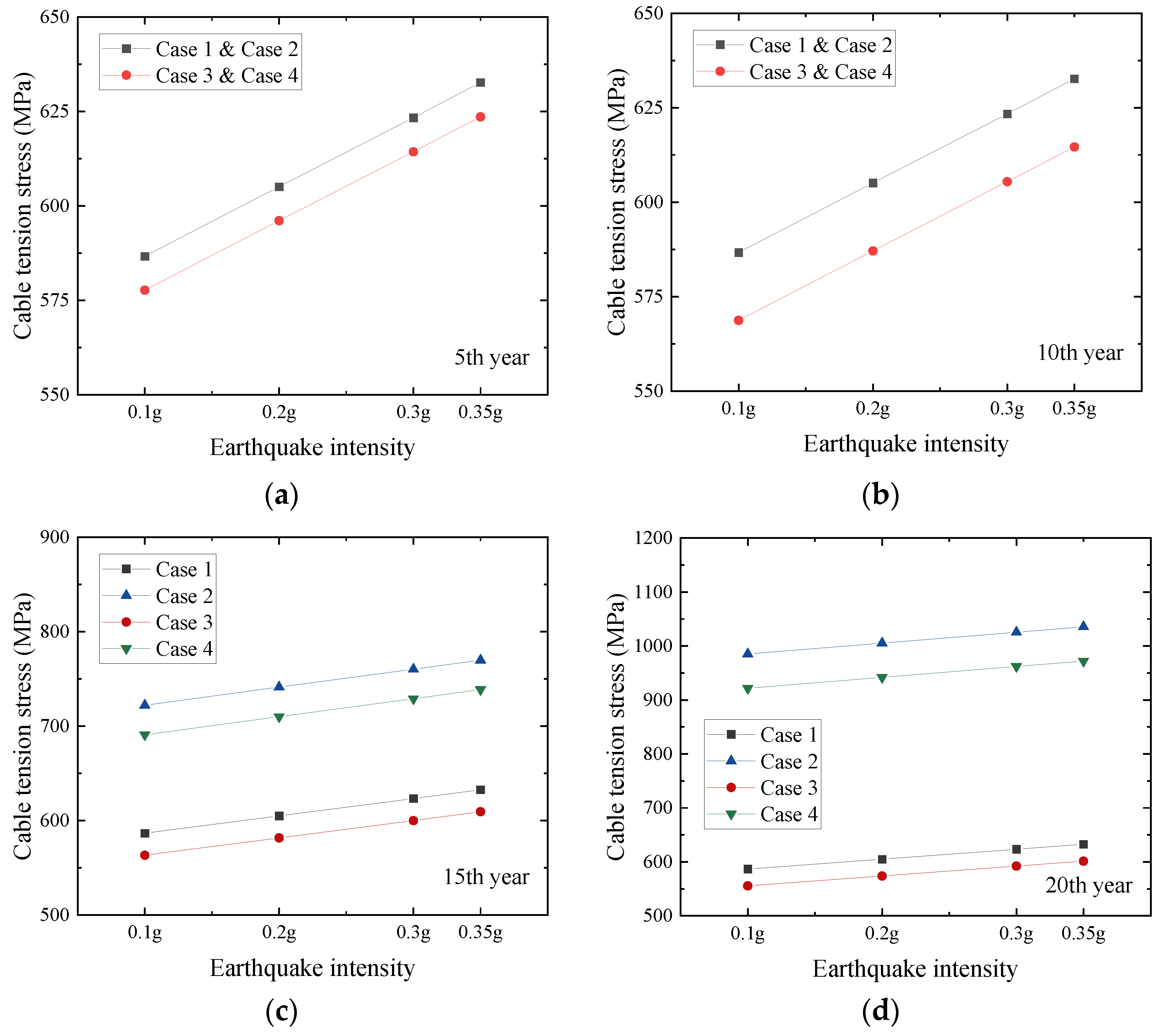
Taking the S1 stay cable as an example, the maximum stress values under different working conditions in various years are illustrated in Figure 12.
Comparing the other stay cables in turn, it was found that the following applied for a single stay cable:
(1) Corrosion has a great adverse effect on the cable stress of stay cables;
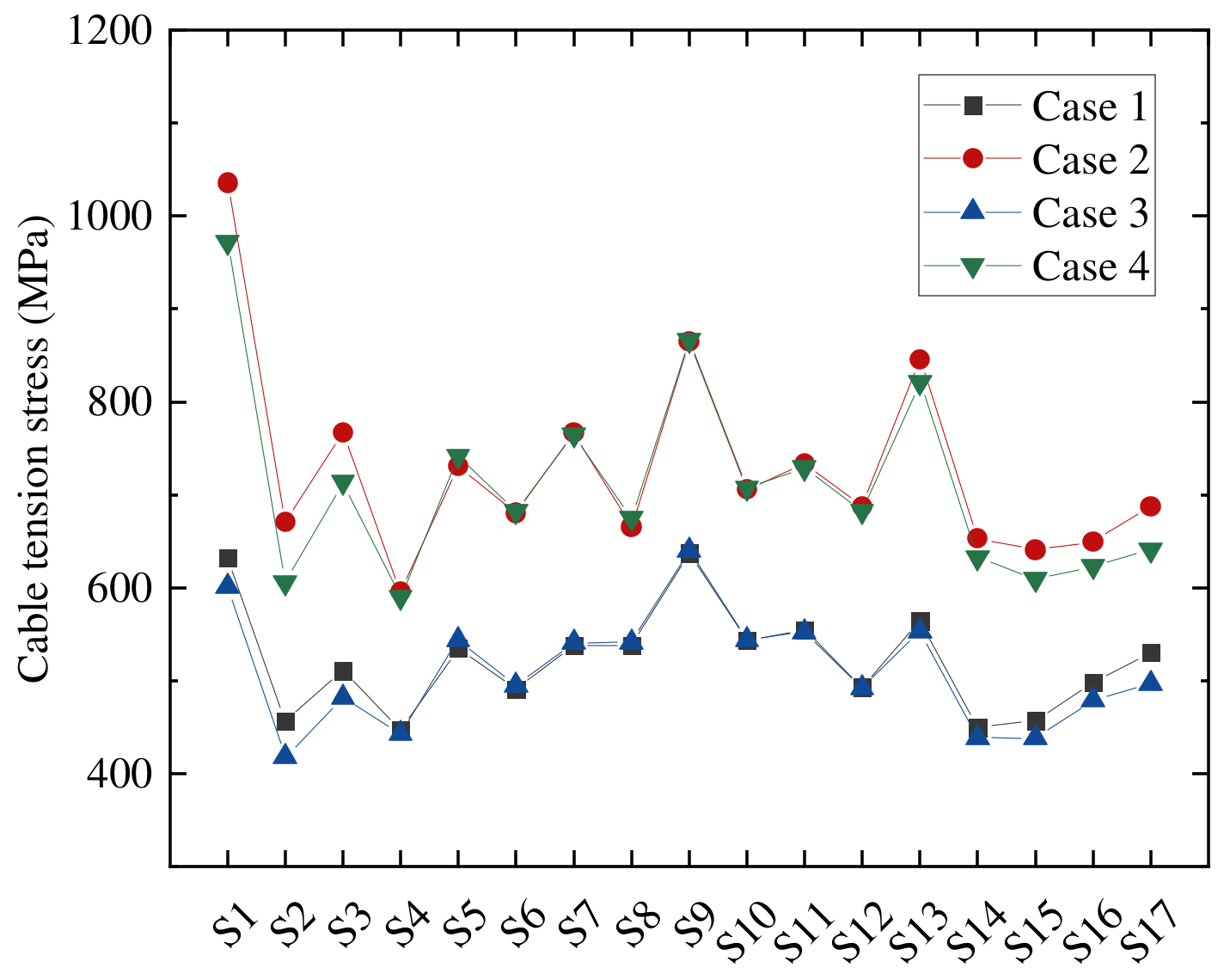
(2) In most cases, the relaxation of the cable force is beneficial to reducing the seismic stress of the cable. However, considering the influence of change in the cable force on the overall deformation of the cable-stayed bridge during earthquakes, as shown in Figure 13, and taking the maximum value of the cable tensile stress under the 0.35 g earthquake intensity in the 20th year as an example, in the middle of a single span, the attenuation of the cable force is not all beneficial to the tensile stress, and there are some adverse changes in the cable tensile stress, such as in cable S5, so it is necessary to prevent possible damage risks.
The tensile strength of each stay cable is 1670 Mpa. According to the design specifications, under the action of the most adverse standard value load combination, the tensile stress of the stay cable is less than 40% of its ultimate strength [28]. When the tensile stress of the cable exceeds 668 Mpa, it is considered that the stay cable has a risk of damage.
According to the statistics of the number of stay cables with damage risk, it was found that under the Case 1 condition, the number of stay cables with damage risk under different seismic intensities is zero, without considering the corrosion of the stay cables and the change in cable force. Under the condition of Case 3, only the gradual attenuation of cable force is considered, and the number of cables with damage risks is zero. Under the condition of Case 2, which only considers the corrosion of stay cables, the reduction in the effective area of stay cables greatly increases the risk of damage to the stay cables. Compared to the Case 2 condition, Case 4 additionally considers the change in the cable force of the stay cables, and the damage risk to the stay cables is relatively reduced. The numbers of stay cables with damage risk under the conditions of Cases 2 and 4 are shown in Table 6.
3.3. Seismic-Response Results for Main-Beam Displacement
Based on the seismic time-history analysis under various working conditions, it was discovered that the cable force and the degree of corrosion of the stay cables have a certain impact on the displacement of the main beam.
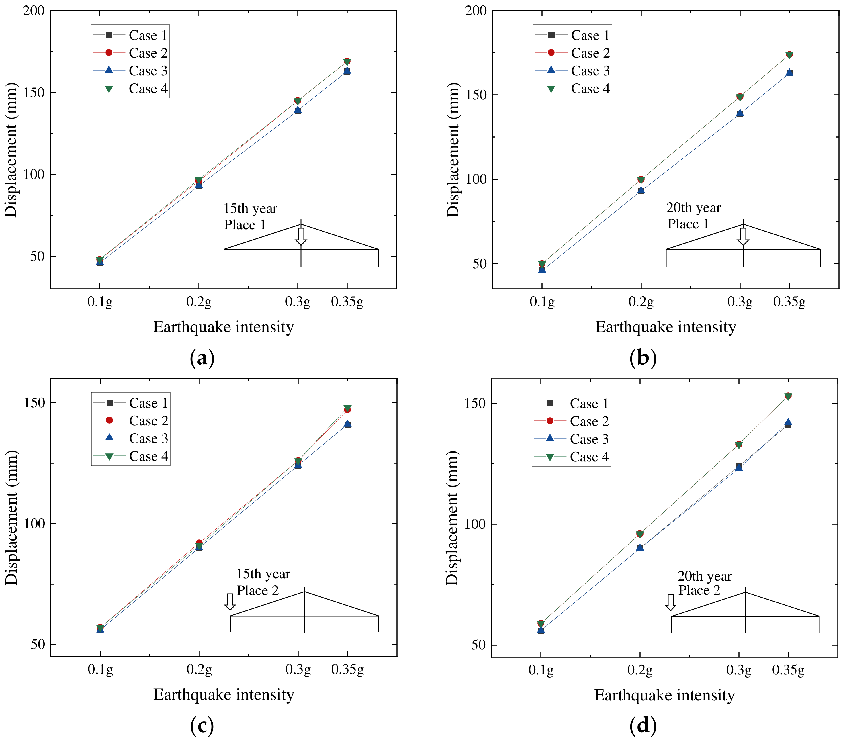
In terms of the longitudinal displacement of the main beam, variations in the cable force have virtually no impact, and the corrosion of the stay cables has a more significant effect. Since it is assumed that the stay cables do not corrode in the first 10 years, the longitudinal displacement of the main beam under different conditions remains almost identical during this period. Therefore, differences in the longitudinal displacement of the main beam under various conditions can be observed in the 15th and 20th years. Figure 14 illustrates the longitudinal displacement of the main beam in the 15th and 20th years under different conditions. The main tower location is denoted as Place 1, and the auxiliary pier location is denoted as Place 2. In the 15th year, the impact of corrosion on the longitudinal displacement of the main beam remained inconspicuous. However, as the extent of corrosion deepened, by the 20th year, it became evident that the corrosion of the stay cables had a significant influence on the longitudinal displacement of the main beam.
The results also found that the corrosion of the stay cables and the changes in cable force in Place 1 and Place 2 have little effects on the transverse displacement of the main beam under different working conditions.
Both changes in the cable force and corrosion have an impact on the vertical displacement of the main beam. Due to the fact that the cable body did not undergo corrosion in the first 10 years of the task, and that the degree of change in the cable force of the stay cable was relatively small, according to the results of the FE simulation, the difference in the vertical displacement of the main beam is small under different working conditions, and the change is more significant in the 15th and 20th years. The maximum displacement change in the positive vertical direction is shown in Figure 15a,b, while the maximum displacement change in the negative vertical direction is shown in Figure 15c,d. The corrosion of the stay cables has a relatively small impact on displacement, which is not beneficial for positive vertical displacement and is beneficial for negative vertical displacement. The influence of the variations in the force of the stay cables on displacement is significant. Owing to the effect of gravity, changes in the force of the stay cables are advantageous for displacement in the positive vertical direction and disadvantageous for displacement in the negative vertical direction. Compared to traditional analytical methods that consider only the corrosion conditions of stay cables, it is observable that, when both the cable corrosion and variation in cable force are considered, under an earthquake intensity of 0.1 g, the negative vertical displacement of the main beam increases by 164.9%. Under an earthquake intensity of 0.35 g, the displacement increases by 29.7%. To prevent the bending failure of the main beam, it is necessary to consider the combined effects of changes in cable force, stay-cable corrosion, and their impact on the negative vertical displacement of the main beam during an earthquake.
In summary, the variation in the force of stay cables has a minimal impact on the seismic displacement of the main beam in both the longitudinal and transverse directions of the bridge. The corrosion of the stay cables hardly affects the transverse seismic displacement of the main beam but has a certain degree of impact on the longitudinal seismic displacement. Therefore, it is necessary to be vigilant against the potential increase in the longitudinal displacement of the main beam caused by the corrosion of the stay cables, as well as against the potential risk of the beam falling. The corrosion and force variation in the stay cables significantly affect the vertical displacement of the main beam. Specifically, the corrosion of the stay cables is more detrimental to the positive vertical displacement, while the variation in cable force is more detrimental to the negative vertical displacement. Compared to the effects of corrosion, the impact of cable-force variation is more significant. Hence, it is essential to consider the effects of force variation, cable corrosion, and their combined effects on the vertical displacement of the main beam during seismic events, with caution toward the risk of the bending failure of the main beam.
4. Conclusions
This study introduces an LSTM-SARIMA combined model for predicting the future trends of cable forces in stay cables based on monitoring data. An FE model was developed to examine the changes in cable stress and main-beam displacement during earthquakes in a cross-sea cable-stayed bridge. The key findings of this research work are summarized as follows:
- (1)
- The results suggest that the LSTM model proficiently addresses missing data during the monitoring of stay cables, ensuring comprehensive data coverage. Furthermore, the SARIMA model accurately predicted the long-term trend of stay-cable-force-detection data, revealing a discernible decline in the force exerted on stay cables over time. The findings indicate that the LSTM-SARIMA model predicted an average decrease of 11.81% in the cable force of the cable-stayed bridge after 20 years;
- (2)
- The corrosion of stay cables has a significant adverse effect on the maximum stress in the stay cables during seismic events. Considering the corrosion of stay cables, the risk of damage to them and the main beam during earthquakes increases. Under an earthquake intensity of 0.35 g in the 20th year, 70.59% of the stay cables’ maximum stress values exceeded the maximum stress values stipulated by the design specifications. Compared to Case 1, where there is no risk of damage, the number of stay cables at risk of damage has substantially increased;
- (3)
- The relaxation of cable forces in cable-stayed bridges predominantly exerts an adverse impact on the negative vertical displacement of the main girder during seismic events. Under a seismic intensity of 0.35 g in the 20th year, the negative vertical displacement increases by 19.6% compared to in Case 1. The cable-force relaxation of stay cables has a minor impact on the displacement of the main beam in both the transverse and longitudinal directions of the bridge;
- (4)
- The detrimental effects of seismic activity on cable-stayed bridges, caused by variations in cable forces and corrosion, are partly mitigated by each other. However, when comparing the seismic response that accounts for both cable corrosion and force variations with traditional analysis methods that only consider corrosion, there remains a significant discrepancy. Particularly notable is the negative vertical displacement of the main beam, which exhibits a variation of 29.7% under a seismic intensity of 0.35 g in the 20th year. Therefore, it is essential to consider both cable corrosion and force variations simultaneously, as the seismic response under these conditions more closely approximates real operational circumstances.
In future studies, the accuracy of the predictive models can be further assessed and validated based on monitoring data collected over the next few years.
Author Contributions
P.L.: conceptualization, methodology and resources; Z.L.: software, visualization, validation and writing—original draft; T.Z.: supervision, funding acquisition and writing—review and editing. All authors have read and agreed to the published version of the manuscript.
Funding
This research was funded by the Hainan Provincial Natural Science Foundation of China (Grant No. 520QN232) and the Graduate Innovation Research Project of Hainan Province (Qhys2023-126).
Data Availability Statement
The original contributions presented in the study are included in the article, further inquiries can be directed to the corresponding author.
Conflicts of Interest
The authors declare no conflicts of interest.
References
- JT/T 1037—2022; Technical Specifications for Structural Monitoring of Highway Bridges. China Architecture & Building Press: Beijing, China, 2022.
- Chen, Z.-W.; Chang, J. Application of Integrated Ridge Regression and SARIMA Methods in the Analysis of Bridge Health Monitoring Data. Sci. Technol. Eng. 2023, 23, 8846–8853. (In Chinese) [Google Scholar]
- Zain, M.; Prasittisopin, L.; Mehmood, T.; Ngamkhanong, C.; Keawsawasvong, S.; Thongchom, C. A Novel Framework for Effective Structural Vulnerability Assessment of Tubular Structures Using Machine Learning Algorithms (GA and ANN) for Hybrid Simulations. Nonlinear Eng. 2024, 13, 20220365. [Google Scholar] [CrossRef]
- Zain, M.; Keawsawasvong, S.; Thongchom, C.; Sereewatthanawut, I.; Usman, M.; Prasittisopin, L. Establishing Efficacy of Machine Learning Techniques for Vulnerability Information of Tubular Buildings. Eng. Sci. 2024, 27, 1008. [Google Scholar] [CrossRef]
- Xu, Y.; Li, Y.; Zheng, X.; Zheng, X.; Zhang, Q. Computer-Vision and Machine-Learning-Based Seismic Damage Assessment of Reinforced Concrete Structures. Buildings 2023, 13, 1258. [Google Scholar] [CrossRef]
- Asgarkhani, N.; Kazemi, F.; Jankowski, R. Machine Learning-Based Prediction of Residual Drift and Seismic Risk Assessment of Steel Moment-Resisting Frames Considering Soil-Structure Interaction. Comput. Struct. 2023, 289, 107181. [Google Scholar] [CrossRef]
- Kazemi, F.; Asgarkhani, N.; Jankowski, R. Machine Learning-Based Seismic Fragility and Seismic Vulnerability Assessment of Reinforced Concrete Structures. Soil Dyn. Earthq. Eng. 2023, 166, 107761. [Google Scholar] [CrossRef]
- Ye, X.-W.; Sun, Z.; Lu, J. Prediction and Early Warning of Wind-Induced Girder and Tower Vibration in Cable-Stayed Bridges with Machine Learning-Based Approach. Eng. Struct. 2023, 275, 115261. [Google Scholar] [CrossRef]
- Hochreiter, S.; Schmidhuber, J. Long Short-Term Memory. Neural Comput. 1997, 9, 1735–1780. [Google Scholar] [CrossRef] [PubMed]
- Xu, Z.; Chen, J.; Shen, J.; Xiang, M. Recursive Long Short-Term Memory Network for Predicting Nonlinear Structural Seismic Response. Eng. Struct. 2022, 250, 113406. [Google Scholar] [CrossRef]
- Liu, Y.; Xiang, S.-T.; Wang, D. Real-time evaluation and prediction of spatial temperature field and temperature effect of steel-concrete composite bridge deck system based on BP-LSTM hybrid model. China Civ. Eng. J. 2021, 54, 57–70+78. (In Chinese) [Google Scholar]
- Liu, H.; Ding, Y.; Zhao, H.-W.; Wang, M.; Geng, F. Deep Learning-Based Recovery Method for Missing Structural Temperature Data Using LSTM Network. Struct. Monit. Maint. 2020, 7, 109–124. [Google Scholar] [CrossRef]
- Cheng, J.; Tiwari, S.; Khaled, D.; Mahendru, M.; Shahzad, U. Forecasting Bitcoin Prices Using Artificial Intelligence: Combination of ML, SARIMA, and Facebook Prophet Models. Technol. Forecast. Soc. Chang. 2024, 198, 122938. [Google Scholar] [CrossRef]
- Agyemang, E.F.; Mensah, J.A.; Ocran, E.; Opoku, E.; Nortey, E.N.N. Time Series Based Road Traffic Accidents Forecasting via SARIMA and Facebook Prophet Model with Potential Changepoints. Heliyon 2023, 9, e22544. [Google Scholar] [CrossRef] [PubMed]
- Cui, T.; Shi, Y.; Lv, B.; Ding, R.; Li, X. Federated Learning with SARIMA-Based Clustering for Carbon Emission Prediction. J. Clean. Prod. 2023, 426, 139069. [Google Scholar] [CrossRef]
- Ping, C.-L. Missing Data Imputation in Bridge Health Monitoring System Base on Hybrid Model of SARIMA and Neural Network. Master’s Thesis, Chongqing University, Chongqing, China, 2011. (In Chinese). [Google Scholar]
- Yin, H.-M. Research on State Evaluation Method of Cable Group Based on Spatial Correlation. Master’s Thesis, Harbin Institute of Technology, Harbin, China, 2018. (In Chinese). [Google Scholar]
- Zeng, X.-L. Research on Cable Relevance Based on Grey Relevance Theory. Master’s Thesis, Hubei University of Technology, Wuhan, China, 2019. (In Chinese). [Google Scholar]
- Iordachescu, M.; Valiente, A.; De Abreu, M. Damage Tolerance and Failure Analysis of Tie-down Cables after Long Service Life in a Cable-Stayed Bridge. Eng. Fail. Anal. 2021, 125, 105437. [Google Scholar] [CrossRef]
- Yuan, Y.; Liu, X.; Pu, G.; Wang, T.; Zheng, D. Temporal and Spatial Variability of Corrosion of High-Strength Steel Wires within a Bridge Stay Cable. Constr. Build. Mater. 2021, 308, 125108. [Google Scholar] [CrossRef]
- Jiang, C.; Wu, C.; Jiang, X. Experimental Study on Fatigue Performance of Corroded High-Strength Steel Wires Used in Bridges. Constr. Build. Mater. 2018, 187, 681–690. [Google Scholar] [CrossRef]
- Lu, W.; He, Z. Effect of Uncertainties in Cable Corrosion and Material Strength on Seismic Fragility of Long-Span Cable-Stayed Bridges in Marine Environments. Structures 2024, 62, 106274. [Google Scholar] [CrossRef]
- De La Fuente, D.; Díaz, I.; Simancas, J.; Chico, B.; Morcillo, M. Long-Term Atmospheric Corrosion of Mild Steel. Corros. Sci. 2011, 53, 604–617. [Google Scholar] [CrossRef]
- Klinesmith, D.E.; McCuen, R.H.; Albrecht, P. Effect of Environmental Conditions on Corrosion Rates. J. Mater. Civ. Eng. 2007, 19, 121–129. [Google Scholar] [CrossRef]
- Lu, W.; He, Z. Vulnerability and Robustness of Corroded Large-Span Cable-Stayed Bridges under Marine Environment. J. Perform. Constr. Facil. 2016, 30, 04014204. [Google Scholar] [CrossRef]
- Ansys Help. Available online: https://ansyshelp.ansys.com/ (accessed on 1 April 2024).
- Wang, H.; Chen, C.; Xing, C.; Li, A. Influence of Structural Parameters on Dynamic Characteristics and Wind-Induced Buffeting Responses of a Super-Long-Span Cable-Stayed Bridge. Earthq. Eng. Eng. Vib. 2014, 13, 389–399. [Google Scholar] [CrossRef]
- JTG/T3365-01-2020; Specifications for Design of Highway Cable-Stayed Bridge. China Architecture & Building Press: Beijing, China, 2020.
- Bao, X.-P. Cable’s Seismic Vulnerability in Cable-Stayed Bridges under Corrosive Service Environment. Master’s Thesis, Dalian University of Technology, Dalian, China, 2014. (In Chinese). [Google Scholar]
- Xu, J.; Chen, W. Behavior of Wires in Parallel Wire Stayed Cable under General Corrosion Effects. J. Constr. Steel Res. 2013, 85, 40–47. [Google Scholar] [CrossRef]
- Zhang, J. Study on Lifetime System Reliability of Long-Span Cable Stayed Bridge under Earthquake Diasaster. Ph.D. Thesis, Southwest Jiaotong University, Chengdu, China, 2018. (In Chinese). [Google Scholar]
Figure 1.
Application process.

Figure 2.
Schematic diagram of cable-stayed bridge. (a) Aerial photograph of the main bridge of a cable-stayed bridge; (b) the schematic diagram of the stay-cable sheathing and steel wires.
Figure 2.
Schematic diagram of cable-stayed bridge. (a) Aerial photograph of the main bridge of a cable-stayed bridge; (b) the schematic diagram of the stay-cable sheathing and steel wires.

Figure 3.
Section diagram of steel box girder.

Figure 4.
FE model of cable-stayed bridge.

Figure 5.
Layout of cable-force sensors for inclined cables.

Figure 6.
Fitting results of LSTM model.

Figure 7.
Comparison of cable-force changes on the broken and opposite sides of the cable.

Figure 8.
Rate of change after cable breakage in inclined cables.

Figure 9.
Long-term trend prediction of cable force for stay cables.

Figure 10.
Corrosion diagram of a stay cable. (a) The entire process curve of diagonal cable corrosion; (b) schematic diagram of the multi-layer arrangement of diagonal cable steel wires.
Figure 10.
Corrosion diagram of a stay cable. (a) The entire process curve of diagonal cable corrosion; (b) schematic diagram of the multi-layer arrangement of diagonal cable steel wires.

Figure 11.
Reduction rate of equivalent-force area of stay cables.

Figure 12.
Tensile stress of stay cables under different working conditions. (a) In the 5th year; (b) in the 10th year; (c) in the 15th year; and (d) in the 20th year.
Figure 12.
Tensile stress of stay cables under different working conditions. (a) In the 5th year; (b) in the 10th year; (c) in the 15th year; and (d) in the 20th year.

Figure 13.
Comparison of stress of stay cables across the entire bridge.

Figure 14.
Longitudinal displacement of the main beam. (a) Place 1 in the 15th year; (b) Place 1 in the 20th year; (c) Place 2 in the 15th year; and (d) Place 2 in the 20th year.
Figure 14.
Longitudinal displacement of the main beam. (a) Place 1 in the 15th year; (b) Place 1 in the 20th year; (c) Place 2 in the 15th year; and (d) Place 2 in the 20th year.

Figure 15.
Vertical negative displacement of the main beam under different working conditions. (a) Positive displacement in the 15th year; (b) positive displacement in the 20th year; (c) negative displacement in the 15th year; and (d) negative displacement in the 20th year.
Figure 15.
Vertical negative displacement of the main beam under different working conditions. (a) Positive displacement in the 15th year; (b) positive displacement in the 20th year; (c) negative displacement in the 15th year; and (d) negative displacement in the 20th year.


Table 1.
Constraint methods for the cable-stayed bridge.
| Types of Bridge Components | Finite-Element Type | Specific Type of Element |
|---|---|---|
| Main beam | Beam element | Beam188 |
| Main tower | Beam element | Beam188 |
| Auxiliary pier | Beam element | Beam188 |
| Stayed cable | Link element | Link10 |
| Rigid beam | Beam element | Beam188 |
| Added mass | Mass element | Mass21 |
| Fluid viscous damper | Combined elements | Combin14 |
| Steel bearings | Combined elements | Combin40 |
Table 2.
Constraint methods for the cable-stayed bridge.
| Place | Longitudinal Bridge Direction | Transverse Bridge Direction | Vertical Direction |
|---|---|---|---|
| Main tower | Damping constraint | Damping constraint | Constraint |
| Auxiliary pier | Release | Damping constraint | Constraint |
Table 3.
Prediction of cable force of stay cables over the next 20 years.
| Prediction Value (kN) | 0 Year | 5th Year | 10th Year | 15th Year | 20th Year |
|---|---|---|---|---|---|
| S1 | 3158 | 3077 | 2995 | 2914 | 2833 |
| S2 | 1443 | 1370 | 1298 | 1225 | 1153 |
| S3 | 1591 | 1520 | 1449 | 1377 | 1306 |
| S4 | 1792 | 1721 | 1649 | 1578 | 1506 |
| S5 | 2164 | 2107 | 2050 | 1993 | 1936 |
| S6 | 2208 | 2135 | 2063 | 1990 | 1917 |
| S7 | 2430 | 2357 | 2284 | 2211 | 2138 |
| S8 | 2623 | 2546 | 2469 | 2392 | 2315 |
| S9 | 3460 | 3379 | 3299 | 3218 | 3137 |
| S10 | 2877 | 2798 | 2719 | 2640 | 2560 |
| S11 | 3000 | 2921 | 2842 | 2763 | 2684 |
| S12 | 3099 | 3020 | 2941 | 2863 | 2784 |
| S13 | 3762 | 3674 | 3585 | 3497 | 3409 |
| S14 | 3117 | 3039 | 2962 | 2884 | 2806 |
| S15 | 3089 | 3009 | 2929 | 2850 | 2770 |
| S16 | 3800 | 3720 | 3640 | 3560 | 3480 |
| S17 | 3841 | 3745 | 3648 | 3552 | 3456 |
Table 4.
Reduction rate of the effective stress area during the corrosion stage of steel-wire substrate.
Table 4.
Reduction rate of the effective stress area during the corrosion stage of steel-wire substrate.
| Time (Year) | 1 | 2 | 3 | 4 | 5 | 6 | 7 | 8 | 9 | 10 |
|---|---|---|---|---|---|---|---|---|---|---|
| S1 | 0.048 | 0.095 | 0.142 | 0.188 | 0.233 | 0.278 | 0.322 | 0.364 | 0.405 | 0.445 |
| S2 | 0.039 | 0.078 | 0.115 | 0.153 | 0.190 | 0.226 | 0.261 | 0.296 | 0.330 | 0.363 |
| S3 | 0.041 | 0.082 | 0.122 | 0.162 | 0.201 | 0.239 | 0.277 | 0.314 | 0.350 | 0.385 |
| S4 | 0.032 | 0.063 | 0.094 | 0.125 | 0.155 | 0.184 | 0.213 | 0.241 | 0.269 | 0.296 |
| S5 | 0.036 | 0.071 | 0.106 | 0.140 | 0.173 | 0.206 | 0.239 | 0.271 | 0.302 | 0.332 |
| S6 | 0.039 | 0.077 | 0.115 | 0.152 | 0.188 | 0.224 | 0.259 | 0.294 | 0.327 | 0.360 |
| S7 | 0.041 | 0.081 | 0.121 | 0.160 | 0.199 | 0.237 | 0.274 | 0.310 | 0.346 | 0.380 |
| S8 | 0.028 | 0.055 | 0.082 | 0.109 | 0.135 | 0.160 | 0.186 | 0.210 | 0.234 | 0.258 |
| S9 | 0.036 | 0.071 | 0.106 | 0.140 | 0.173 | 0.206 | 0.238 | 0.269 | 0.299 | 0.329 |
| S10 | 0.032 | 0.063 | 0.094 | 0.125 | 0.155 | 0.184 | 0.213 | 0.241 | 0.268 | 0.295 |
| S11 | 0.033 | 0.065 | 0.097 | 0.128 | 0.159 | 0.189 | 0.218 | 0.247 | 0.275 | 0.302 |
| S12 | 0.037 | 0.073 | 0.109 | 0.145 | 0.179 | 0.213 | 0.247 | 0.279 | 0.311 | 0.341 |
| S13 | 0.041 | 0.082 | 0.122 | 0.162 | 0.201 | 0.239 | 0.276 | 0.312 | 0.347 | 0.381 |
| S14 | 0.037 | 0.074 | 0.110 | 0.145 | 0.180 | 0.214 | 0.247 | 0.280 | 0.312 | 0.343 |
| S15 | 0.037 | 0.073 | 0.109 | 0.144 | 0.179 | 0.213 | 0.246 | 0.278 | 0.310 | 0.341 |
| S16 | 0.031 | 0.062 | 0.093 | 0.123 | 0.152 | 0.181 | 0.209 | 0.236 | 0.263 | 0.289 |
| S17 | 0.032 | 0.063 | 0.093 | 0.123 | 0.152 | 0.181 | 0.209 | 0.236 | 0.263 | 0.289 |
Table 5.
Working conditions of seismic-response analysis.
| Case | Considering Changes in Cable Force | Considering Corrosion of Stay Cables |
|---|---|---|
| Case 1 | × | × |
| Case 2 | × | √ |
| Case 3 | √ | × |
| Case 4 | √ | √ |
Table 6.
Case 1: Number of inclined cables at risk of damage under different earthquake intensities.
Table 6.
Case 1: Number of inclined cables at risk of damage under different earthquake intensities.
| Service Time | Case | Earthquake Intensity | |||
|---|---|---|---|---|---|
| 0.1 g | 0.2 g | 0.3 g | 0.35 g | ||
| 0~10th year | Case 2 | 0 | 0 | 0 | 0 |
| Case 4 | 0 | 0 | 0 | 0 | |
| 15th year | Case 2 | 4 | 4 | 8 | 12 |
| Case 4 | 4 | 8 | 8 | 8 | |
| 20th year | Case 2 | 20 | 28 | 40 | 48 |
| Case 4 | 12 | 28 | 32 | 44 | |
Disclaimer/Publisher’s Note: The statements, opinions and data contained in all publications are solely those of the individual author(s) and contributor(s) and not of MDPI and/or the editor(s). MDPI and/or the editor(s) disclaim responsibility for any injury to people or property resulting from any ideas, methods, instructions or products referred to in the content. |
© 2024 by the authors. Licensee MDPI, Basel, Switzerland. This article is an open access article distributed under the terms and conditions of the Creative Commons Attribution (CC BY) license (https://creativecommons.org/licenses/by/4.0/).
Share and Cite
MDPI and ACS Style
Lu, P.; Liu, Z.; Zhang, T. A Machine Learning Model to Predict the Seismic Lifecycle Behavior of a Cross-Sea Cable-Stayed Bridge. Buildings 2024, 14, 1190. https://doi.org/10.3390/buildings14051190
AMA Style
Lu P, Liu Z, Zhang T. A Machine Learning Model to Predict the Seismic Lifecycle Behavior of a Cross-Sea Cable-Stayed Bridge. Buildings. 2024; 14(5):1190. https://doi.org/10.3390/buildings14051190
Chicago/Turabian StyleLu, Ping, Zichuan Liu, and Tianlong Zhang. 2024. "A Machine Learning Model to Predict the Seismic Lifecycle Behavior of a Cross-Sea Cable-Stayed Bridge" Buildings 14, no. 5: 1190. https://doi.org/10.3390/buildings14051190
Note that from the first issue of 2016, this journal uses article numbers instead of page numbers. See further details here.