
Research on Complex Network Models and Characteristics of Building Material Enterprises Based on Competitive Relationships

School of Civil Engineering, North China University of Technology, Beijing 100144, China
*
Author to whom correspondence should be addressed.
Buildings 2024, 14(5), 1192; https://doi.org/10.3390/buildings14051192
Submission received: 19 February 2024
/
Revised: 26 March 2024
/
Accepted: 31 March 2024
/
Published: 23 April 2024
(This article belongs to the Section Construction Management, and Computers & Digitization)
Abstract
:Based on complex network theory, this paper establishes a Boolean competitive relationship network model and a weighted competitive relationship network model for building material enterprises based on big data and performs empirical analyses with construction prefabricated component (PC) enterprises in the Beijing–Tianjin–Hebei region as research samples. Results show the competitive relationship network of PC enterprises in the Beijing–Tianjin–Hebei region is characterised by the development of a small-world network, and its cumulative degree and out-degree (in-degree) intensity distributions are single-scale networks with fast-decaying tails. The network has strong network clustering and assortativity, and it can truly reflect the competitive status and dynamics of the enterprises.
1. Introduction
The construction supply chain involves the flow of materials, information, and capital through various components of a construction project. The construction supply chain is a complex, large system that includes multiple participants such as building material suppliers, manufacturers, contractors, distributors, and logistics companies [1]. In the new digital era of escalating demand from construction clients, the building material enterprises are increasingly characterised by competition [2]. In addition, according to China’s Statistical Analysis of the Development of the Construction Industry 2022, the number of construction enterprises has continued to increase yearly; by the end of 2022, the total of number of construction enterprises nationwide is 143,621, with fierce competition amongst them. Although the building material enterprises feel strong competitive pressure in practice, they are not clear about who their competitors are, and they lack a basic understanding of how to cope with the fierce competitive environment and develop.
A complex network is an abstract model for understanding real-world complex systems. A complex network abstracts entities in complex systems as nodes and relationships between entities as connectivity. Since 2000, complex network research has been rapidly applied to practical areas such as computer networks [3,4,5], biological networks [6,7,8], technological networks [9,10,11], brain networks [12,13,14], climate networks [15,16,17] and social networks [18,19,20]. Competitive relationships are pervasive in the real world, such as species competition in ecosystems, corporate competition in economic markets and individual competition in social networks. The study of competitive relationships can improve the understanding and explain the behavioural evolution of these complex systems, predict and manage competitive behaviour in complex systems, and optimise resource allocation and decision making. In existing studies, the research on complex networks based on competitive relationships is mainly conducted for industries such as logistics [21,22,23], manufacturing [24,25], and software [26,27], and they mostly use enterprises as nodes and competitive relationships between enterprises as edges to construct complex network models. Furthermore, some scholars construct complex networks with countries as nodes and trade rivalries as edges, such as Long et al. [28] and Wang et al. [29].
The competitive relationship between enterprises is primarily defined the derivation of the concept of niche overlap [30], which states that competition exists between enterprises when they compete for limited market resources, human resources, and capital resources. Thus, firms’ competitive relationships can be defined as follows: (a) Competitive relationships arise when firms have similar products, which follows Watts et al.’s [31] definition, namely, to take a dichotomous network model of component firms and products, and then convert it into a model of competitive network relationships between firms [32,33]. (b) The competitive relationship between firms is defined in terms of two dimensions: homogeneous products and the geographic location of firms. For example, Hou et al. [34] defined the competitive relationship between logistics firms based on two dimensions: the type of service and the geographical location of the logistics service provided by the logistics firms. Gao et al. [35] argued that a competitive relationship exists between the community of logistics enterprises in the same region or neighbouring regions with the same type of business operation; they provided a method for calculating the degree of market commonality of logistics enterprises in the same region and neighbouring regions. In addition, George [36] suggested that in the same competitive field, firm i will try to avoid competing with rival j whose market share is 50% higher. Zhu et al. [37] used this approach to model the network of competitive relationships in the property and casualty insurance industry.
Building material enterprises play a remarkable role as crucial entities within the construction supply chain. Conducting qualitative and quantitative analyses of the market-competition status of these enterprises is a vital prerequisite for optimising the resilience of the construction supply chain. However, compared with other types of enterprises, building material enterprises often face unique challenges due to the varying service radii of different materials, hampering the qualitative and quantitative study of their competitive relationships. To date, few scholars have embarked on research in this area. This paper aims to analyse the market-competition status of building material enterprises qualitatively and quantitatively. Drawing on previous research achievements in enterprise competition relationships and the application status of complex network theory, this paper focuses on building material enterprises, considering factors such as geographic location, service radius, and theoretical market size to explore the mechanisms and calculation methods for defining competitive relationships and intensity. Based on complex network theory and using enterprise transaction data as a foundation, this paper constructs a Boolean (unweighted and symmetric) competitive relationship network model, with enterprises as nodes and competition relationships as edges, as well as a weighted competitive relationship network (WCRN) model, with enterprises as nodes and competition intensity as edge weights. This approach achieves the objective of quantitative and qualitative analyses of the market competition status of building material enterprises. This paper offers new perspectives and methods for the study of competitive relationships amongst enterprises within the construction supply chain. Further, this paper adopts prefabricated component (PC) enterprises as the subject for empirical research. Using web-crawling techniques, this paper collects data on bid wins by building PC enterprises and their actual geographical distribution in the Beijing–Tianjin–Hebei region from 2016 to 2022. This paper constructs the Boolean competitive relationship network (BCRN) and the WCRN of PC enterprises in the Beijing–Tianjin–Hebei region for 2016–2020. This paper facilitates the qualitative and quantitative analyses of the market competition status of PC enterprises in the Beijing–Tianjin–Hebei region, thereby verifying the effectiveness of the model.
The key issues addressed in this paper include (a) investigating the mechanisms and calculation methods for defining the competitive relationships and intensity amongst building material enterprises and (b) quantifying the market competition pressure between building material enterprises, breaking through the limitations of previous purely qualitative research. The innovative aspects of this research are (a) constructing a dynamic competition model for building material enterprises based on complex network theory and (b) fully considering the characteristics of construction enterprises when studying the construction mechanism of competitive relationship networks, making their service radius an important factor in defining competitive relationships.
2. Modelling
2.1. Competitive Relationships
Firstly, the geographical region where a firm is located decides the amount of resources it can compete for. In this paper, regarding the definition of the competitive relationship between enterprises in the nodes of the construction supply chain, the service radius is a very typical characteristic of the enterprise, and is determined by the size of the enterprise. Moreover, the enterprise’s product supply capacity is largely dependent on the service radius, which has a strong spatial distribution characteristic. Therefore, the competitive relationship between node enterprises should firstly be expressed as whether the region where the service radius of the enterprise is located is cross. If the node enterprises have the same demand side or target customers within their respective service radii, then a competitive relationship exists amongst the enterprises.
Secondly, the bidding owner pays great attention to the overall scale strength of the bidding party in the bidding. They review the overall qualifications of the bidders, and different project sizes require that the qualifications of the bidders are not the same. Usually, the bidding enterprises involved in the same project are similar in size. When defining the competitive relationship in this paper solely through George’s theory, the leading or monopolistic enterprises in the market have a large difference in market share with other enterprises. This kind of enterprise is shown as an isolated node in the network by defining the competitive relationship in this manner, and it is not conducive to the analysis of the overall competitive relationship in the market. Therefore, in this paper, based on George’s theory, the theoretical market share is replaced with the theoretical market (the amount of supply required by all the demanders within the service radius) within the service radius and stipulates that firms do not compete with firms with more than 50% of their theoretical market share.
Figure 1 shows the specific process of defining competitive relationships.
(1) If the areas included in the service radii of building material enterprises i and j do not overlap, their customer goals are completely different, and they have no competitive relationship, that is, wij = wji = 0, where wij is the intensity of competition given by enterprise i to enterprise j, that is, the competitive pressure that enterprise j feels from enterprise i; wji is the intensity of competition that enterprise j gives to enterprise i, that is, the competitive pressure that enterprise i feels from enterprise j.
(2) If the areas included in the service radius of building material enterprises i and j are completely coincident, their customer goals are exactly the same. Combined with George’s theory, when the theoretical market of enterprises i and j are less than 50%, the competition intensity is 1, that is, wij = wji = 1. When the theoretical markets of enterprises i and j are ≥50%, although enterprises i and j have the same target customers, they have no competitive relationship due to the large gap in the theoretical market, that is, wij = wji = 0.
(3) If the areas included in the service radius of the building material enterprises i and j intersect, then combined with George’s theory, when the theoretical market of enterprises i and j are less than 50%, the competition intensities are wij and wji, respectively. When the theoretical markets of enterprises i and j are ≥50%, although they have the same target customers, they have no competitive relationship due to the large gap in the theoretical market, that is, wij = wji = 0.
2.2. Complex Network Modelling
2.2.1. Boolean Competitive Relationship Network Model
Taking an enterprise in the construction supply chain as a node, two enterprises are connected to form an edge when the ranges covered by their respective service radii intersect and the theoretical market difference is less than 50%. According to the above rules, a BCRN model is constructed. The set of BCRN is expressed as G = (F, A), where F is the set of node firms in the construction supply chain, and A is the adjacency matrix of the competitive relationships between node firms in the construction supply chain.
2.2.2. Weighted Competitive Relationship Network Model
BCRN only considers whether a competitive relationship exists between the firms in the construction supply chain and how many competitors the firms face; it does not consider the intensity of competition in the market. Grasping the intensity of business competition amongst firms in the construction supply chain to develop a competitive strategy is even more relevant. In this paper, the intensity of the competitive relationship between firms at the nodes of the construction supply chain is measured by the theoretical market commonality, which is the degree to which firms i and j share the theoretical market. The competitive pressure between firms is quantified based on the concept of theoretical market commonality. Then, a WCRN model is constructed using competitive pressures as side weights. The theoretical market commonality is calculated as shown in Equation (1). The geospatial distance between firms in the construction supply chain is fully considered in determining the theoretical market commonality.
where mij is the theoretical market commonality between firms i and j, seti is the area covered by the service radius of enterprise i, setj is the area covered by the service radius of enterprise j and pij is the demand at any demand point in the region where firms i and j intersect.
where pi is the theoretical market for firm i, and pj is the theoretical market for firm j. Figure 2 shows the detailed model construction.
In Figure 2, rik is the straight-line distance from enterprise i to all demand points k that it can supply, and rjk is the straight-line distance from enterprise j to all demand points k that it can supply.
(a) i and j are any two enterprises, whose service radii are determined and denoted as Ri and Ri, respectively.
(b) According to Ri and Ri, the service areas of the i and j are determined, and the theoretical markets pi and pj within the service radius of i and j are calculated.
(c) The intersection state of the service areas of i and j are determined. If they do not intersect, then no competitive relationship exists between i and j; otherwise, go to the next step.
(d) The market mutuality mij of enterprises i and j is calculated according to Equation (1).
(e) wij and wji are calculated according to Equation (2).
2.3. Comparison with Existing Research
Table 1 shows the comparison between the constructed model of this paper and the existing research results, and it can be found that the research of this paper opens up a new perspective in the study of the competitive relationship of construction enterprises, and at the same time, it enriches the application field of complex networks in the study of the competitive relationship of enterprises.
3. Model Analysis
The main difference between the BCRN and WCRN to be constructed in this paper is that the former builds the network from the number of competitive relationships, whereas the latter mainly establishes the network from the strength of competitive relationships. Thus, the following indicators are introduced to compare and analyse the topological indicators of the model.
3.1. Node Degree and Degree Distribution
Node degree (ND) is an important statistic for Boolean networks. ND is the number of neighbouring edges of a node, as shown in Equation (3).
where ki is the degree of node i, and aij is the matrix element of the adjacency matrix. When a relationship exists between nodes i and j, aij = aji = 1 and 0 otherwise.
In addition, degree distribution is one of the important indicators to describe the network structure. This property is often expressed in terms of the distribution function of the ND P(k) or the cumulative degree distribution function P(>k) [40]. P(k) denotes the ratio of the number of nodes with ND k to the number of all nodes in the network. P(>k) is the probability distribution of nodes with degree not less than k, as described in Equation (4).
According to the findings of Amaral et al. [41]: the ND distribution characteristics in many real networks belong to three types, namely, scale-free network, wide-scale network and single-scale network.
3.2. Node Strength
To describe the weighted network, two important concepts are introduced: edge weight and point weight. Edge weight wij refers to the connection weight of nodes i and j. Point weight represents the node strength (NS), and in an undirected network, the point weight denotes the sum of all edge weights of a node. NS is defined by Equation (5) [42].
Point weights in directed networks are accordingly split into out- and in-degree weights. The out-degree weight of a node is the sum of all edge powers from that point, representing the sum of competitive pressures brought by the firms at that node to the other firms, as defined by Equation (6).
The corresponding total weight is defined by Equation (7).
NS difference is the gap between the out-degree weight and the in-degree weight, which decides the competitive position of the node firm in the market, as defined by Equation (8).
If si(Δ) > 0, node enterprise i brings competitive pressure to its neighbouring enterprises and has a competitive advantage. If si(Δ) ≤ 0, node enterprise i is mainly under the pressure of its neighbouring enterprises and does not have a competitive advantage.
3.3. Average Nearest-Neighbour Degree
ND only represents the number of adjacent edges to node i. However, even if some nodes have the same ND in the network structure, their positions in the network are dissimilar due to the different connectivity of adjacent edge nodes. Average nearest-neighbour degree (ANND) refers to the average degree of nodes adjacent to node i, which can measure how connected the neighbours of node i are in the network, as defined by Equation (9).
where v(i) is the set of all neighbour nodes of node i, and kj is the degree of neighbour j.
The ANND of the network is the mean of the ANND of all nodes, as defined by Equation (10).
3.4. Average Nearest-Neighbour Strengths
By calculating the average of nearest-neighbour strengths (ANNS), the closeness of the connection between the neighbours of a node can be measured. Even if two nodes have the same ANND, their ANNS may be substantially different. The ANNS of node i is defined by Equation (11).
The ANNS of the network is the mean of the ANNS of all nodes, as defined by Equation (12).
3.5. Clustering Coefficient
Clustering coefficient (CC) indicates the clustering of network nodes and describes the proportion of neighbours of nodes in the network that are also neighbours of one another. The CC of node i is the ratio of the number of existing connected edges to the maximum possible number of connected edges amongst all its neighbours. The CC of node i is defined by Equation (13).
where ki is the degree of node i, li is the number of connected edges between the neighbours of node i and cci is the CC of node i.
The CC of the network is the mean of the CC of all nodes, as defined by Equation (14).
3.6. Weighted Clustering Coefficient
If border weighted are considered, the weighted clustering coefficient (WCC) of node i is defined by Equation (15).
where wij is the edge weight of nodes i and j, and si is the NS of node i.
The WCC of the network is the mean of the WCC of all nodes, as defined by Equation (16).
3.7. Small World Quotient
This paper uses the ‘Small World Quotient (SWQ)’ proposed by Davis [43] to detect whether BCRN and WCRN have small-world characteristics. The calculation method is as follows:
where C is the average CC of BCRN or WCRN; L is the average path length of BCRN or WCRN; Crandom and Lrandom are the average CC and average path length of random networks, respectively, which have the same number of nodes and average degree as BCRN and WCRN.
If SWO is greater than 1, the network has ‘small world’ characteristics.
4. Empirical Research
4.1. Data Sources
PC is a type of building construction in which building components are prefabricated in a factory or manufacturing site and then assembled and installed on site. Traditional building construction methods usually require many manual operations and cumbersome construction processes on site, which is not only time consuming and labour intensive but also prone to quality problems. The emergence of PC has changed this situation. By standardising production in factories, PCs enable the precise control of processes and quality assurance. Therefore, building PCs have been widely used in the construction industry as a modern way of building construction. As early as 2016, the Chinese government started to promote the development of assembled buildings with the Beijing–Tianjin–Hebei region and other urban agglomerations as pilot areas, aiming to bring the proportion of assembled buildings in new construction to 30% in about 10 years. The national 14th Five-Year Plan further proposed vigorously developing prefabricated buildings. Until now, the assembly building market in the Beijing–Tianjin–Hebei region has a certain scale.
The research data for this paper were sourced from the China Construction Market Supervision Public Service Platform [44], which is an official data website established by the Ministry of Housing and Urban-Rural Development of the People’s Republic of China. It encompasses databases of enterprises, personnel, and projects, as well as a database for enterprise integrity within the construction field across the whole country. The project database includes information such as project names, project addresses, and project bidding information. The data collection process is as follows:
(a) Source Data Acquisition: We used “prefabricated components” as the search term, with the time range set from 2016 to 2022 and the geographical scope limited to the Beijing–Tianjin–Hebei region. Through web crawling, we obtained bid-winning information for a total of 8964 projects. Each project’s bid-winning entry includes information such as the project name, project address, tendering owner, bid-winning date, bid-winning enterprise, and bid-winning amount.
(b) Acquisition of Latitude and Longitude Coordinates: We utilized the Python programming language to call the Google Maps API, obtaining the latitude and longitude coordinates for each project address and bid-winning enterprise.
(c) Data Input: We divided all the bid-winning information from 2016 to 2022 into seven parts by year and input them into the model constructed in Section 2. The data input into the model include project address, project latitude and longitude coordinates, name of the bid-winning enterprise, latitude and longitude coordinates of the bid-winning enterprise, and the bid-winning amount of the project.
4.2. BCRN and WCRN of PC Enterprise
The computational results of the model in this paper are output in the form of matrices, yielding a total of 14 matrices: the Boolean competitive relationship matrix and the weighted competitive relationship matrix for each year from 2016 to 2022. The matrices for the same year have the same order, and the order of the matrices represents the number of enterprises. Table 2 lists the order of matrices for each year, indicating that within the network of competitive relationships among PC component enterprises in the Beijing–Tianjin–Hebei region, there were 12 enterprises in 2016, 37 enterprises in 2017, 54 enterprises in 2018, 397 enterprises in 2019, 568 enterprises in 2020, 323 enterprises in 2021, and 168 enterprises in 2022.
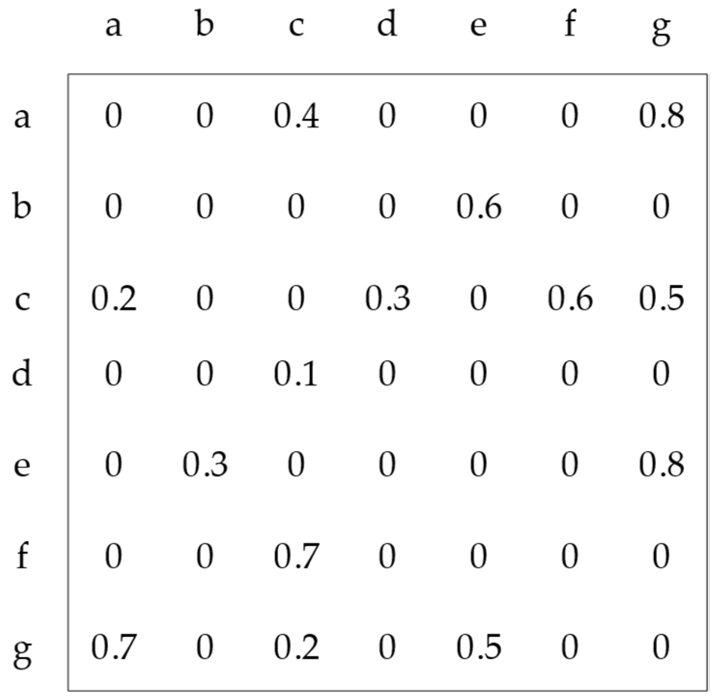
Figure 3 shows a part of the Boolean competitive relationship matrix for the year 2020, where letters a-g represent different enterprises. An element of 1 in the matrix indicates the existence of a competitive relationship, while an element of 0 indicates the absence of such a relationship. Figure 4 presents a part of the weighted competitive relationship matrix for 2020. The elements in the matrix indicate the intensity of competition; for example, wbe = 0.6 indicates the competitive pressure enterprise b places on enterprise e, while web = 0.3 indicates the competitive pressure enterprise e places on enterprise b.
4.2.1. BCRN of PC Enterprise
We use the Boolean competitive relationship matrix for each year as the source data and combine it with the Gephi 0.10.1 software to draw the BCRN graph. Figure 5 shows the BCRN graph for each year from 2016–2022, the nodes in the graph indicate different enterprises, the grey connecting lines indicate the competitive relationships existing between enterprises, the more competitive relationships enterprises have, the larger their node degree is node, and the colour is closer to red.
4.2.2. WCRN of PC Enterprise
Similarly, we use the weighted competitive relationship matrix of each year as the source data and combine it with the Gephi software to draw the WCRN graph, and Figure 6 shows the WCRN graph for each year from 2016 to 2022. The nodes in the graph represent different firms, and the colour of the line connecting the nodes indicates the intensity of competition between firms, and the greater the intensity of competition between firms, the closer the colour of the line is to red.
4.3. Characteristics
4.3.1. Connectivity
- Degree
In the BCRN model of construction-PC firms, the ND represents how many competitors each construction-PC firm has in the study area. Table 1 presents the average degree, maximum value and standard deviation of nodes in the BCRN of PC construction enterprises in the Beijing–Tianjin–Hebei region from 2016 to 2022. The maximum average of ND in BCRN is 142 in 2020, the minimum is 1.8 in 2016 and the average is 402.2. The remaining parameters such as mean, maximum, and standard deviation of ND for each year are shown in Table 3. The average ND of the Boolean competitive network model of construction-PC company i in the study area during 2016–2022 continued to increase until 2020 and then began to decrease; the degree of dispersion of the distribution of the ND in each year is consistent with the trend of the average ND of the network.
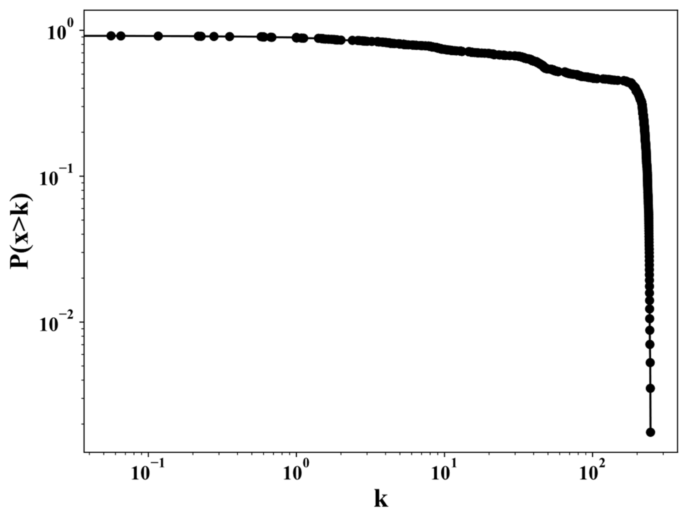
The distribution of node cumulative degree is the same in each year, taking the cumulative degree distribution of the enterprise competition network in 2020 as an example (Figure 7). As the ND k increases, the cumulative degree distribution in 2020 exhibits a rapidly decaying tail, which belongs to a single-scale network.
- 2.
- Node strength
The WCRN is constructed based on the theoretical market commonality, and the NS portrays the competitive intensity of construction-PC firms. Table 4 shows the average, maximum and standard deviation of NS in the WCRN of PC construction enterprises in the Beijing–Tianjin–Hebei region from 2016 to 2022. The maximum NS in 2016 to 2022 is 479.62 in 2020, and the minimum is 6.01 in 2016. The average value of each year increased from 2016 to 2020, reached the maximum value every year, then began to decrease. The increase and decrease trend is consistent with the ND.
Similarly, the cumulative distribution of nodal entry and exit intensities is generally consistent across years. Taking 2020 as an example (Figure 8 and Figure 9), the cumulative in-degree distribution and the cumulative out-degree distribution exhibit rapidly decaying tails, consistent with single-scalar properties.
Figure 10 shows the scatter diagram of the difference in corporate strength in each year. The maximum value of competitive pressure that companies export to the outside world, namely, 65.51, was observed in 2020, and companies were affected by the outside world. The maximum value of competitive pressure is 57, but the overall distribution shows that the distribution of competitive pressure in each year is balanced.
4.3.2. Assortativity
Assortativity refers to the competition amongst enterprises with large NDs. On the contrary, disassortativity refers to enterprises with large NDs competing only with enterprises with small NDs. To study whether the competition network of construction-PC enterprises has assortativity, firstly, the average degree of neighbours of nodes is studied from the perspective of Boolean competition network, and the correlation between this index and ND is analysed.
Table 5 presents the ANND of the BCRN of PC construction enterprises in the Beijing–Tianjin–Hebei region from 2016 to 2022. Table 6 shows the correlation coefficients between the ANND and ND for the BCRN in each year. ANND rose from 2.1 in 2016 to 147 in 2020 and then dropped to 44.5 in 2022. Except for the ND–ANND correlation coefficient in 2016, namely, 0.77, which is lower than 0.9, the correlation coefficients of ND–ANND for the rest of the years are greater than 0.9, and the ND and the average degree of neighbouring points correlation coefficients are large and stable.
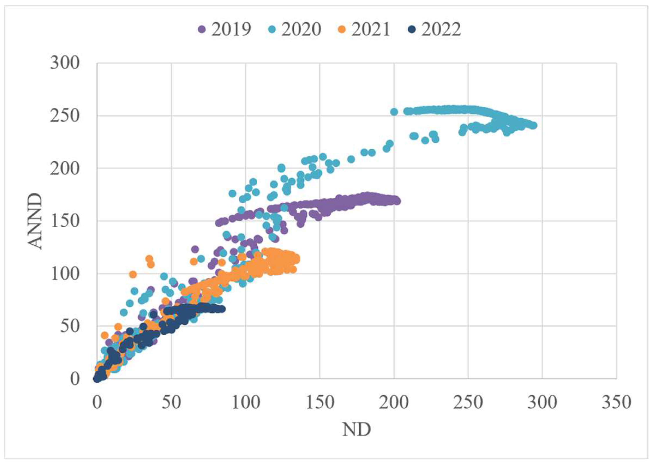
Figure 11 also shows that ND and ANND are linearly distributed, indicating that the competition amongst building PC enterprises in the network model occurs amongst enterprises with similar NDs. The network belongs to assortative network and has strong stability.
Table 7 presents the ANNS of the WCRN of PC enterprises in the Beijing–Tianjin–Hebei region from 2016 to 2022. Table 8 shows the correlation coefficients between the ANNS and the NS for the WCRN in each year. Analysis in terms of a weighted network of competitive relationships leads to the same conclusions as the Boolean competitive network. The change in ANNS of construction-PC companies is similar to that of ANND, which increased from 2016 to 2020 and then began to decrease. The correlation coefficients of NS-ANNS are in the range of 0.82–0.97 during the study period. From the perspective of the WCRN, the results of the competitive relationship network assortativity test of the construction-PC firms are also very satisfactory, and the network has strong assortativity, which can also be illustrated by combining with the NS–ANNS scatter distribution of 2019–2022 in Figure 12.
4.3.3. Clustering
The CC of node i is the ratio of the number of existing connected edges to the maximum possible number of connected edges amongst all its neighbours in the network. which represents the completeness of the network. Analysing the relationship between the CC and the ND reveals the general situation of the competitive relationship between the enterprise group with strong clustering and the enterprise with large ND. Table 9 lists the CC of the BCRN and the WCC of the WCRN of PC enterprises in the Beijing–Tianjin–Hebei region from 2016 to 2022. The network CC is small in 2016 to 2018, all less than 0.5, indicating the network does not have a strong clustering during this period, and the CC is between 0.65 and 0.71 from 2019 to 2022, indicating the network during this period has a certain degree of agglomeration. In addition, the weighted CC of each year is larger than the Boolean CC, indicating the weighted network has higher clustering.
Table 10 shows the correlation coefficients of the CC–ND in BCRN and WCC–NS in WCRN for PC enterprises in the Beijing–Tianjin–Hebei region from 2016 to 2022. During 2016–2022, the correlation coefficients between Boolean network CC and ND, weighted network CC and NS are all positive, the minimum value is 0.40 and the maximum value reaches 0.85. This outcome shows that most construction-PC enterprises have large ND (strength) values, and their clustering is large. For enterprises with large ND (strength) values, the competition between adjacent enterprises is also strong.
4.3.4. Small World
The SWQ of each year is calculated from Equation (17), as shown in Table 11.
The results show that whether for BCRN or WCRN, the SWQ in 2016–2018 is less than 1, which does not have the small-world characteristic, and the SWQ in 2019–2020 is greater than 1, indicating that the competitive relationship network during the period has the small-world characteristic. In 2021–2022, the SWQ of BCRN is greater than 1, but the SWQ of WCRN is less than 1, indicating that when only the number of competitions is considered but not the intensity of competition, the competitive relationship network during the period has small-world characteristics.
5. Economics Explanation
Changes in the topological indicators of the BCRN network can illustrate the evolving characteristics of the competitive relationships of construction-PC firms. From 2016 to 2022, the average ND and its standard deviation of the construction-PC firms in the BCRN became larger from 2016 and then decreased from 2020, suggesting more competitors and greater competition amongst the construction-PC firms, which intensified and peaked in 2020 mainly due to the national policy push. The indicator started to decrease after 2020 because of COVID-19 at the end of 2019, which led to a downturn in the market for construction-PC in the study area and even in the country. Moreover, many companies faced closure because they had not had any order for a long time, and this is why the overall volumes of network modelling for 2021 and 2022 were much smaller than that for 2020. The single-scale characteristic of the cumulative ND distribution shows that when only the number of competitions is considered, the competition pressure heterogeneity level faced by firms in the competition network is high.
WCRN’s NS analysis shows that the construction-PC market in the study area has always maintained a high level of competition even under the influence of COVID-19 when many companies closed and exited the market. However, with COVID-19, a downturn in the overall construction industry market was noted. For the existing companies, the competition did not decrease much. This outcome can also be seen from the scatter plot of enterprise intensity difference. Although the overall volume became smaller after the epidemic, the maximum-pressure output value and the maximum-pressure input value of each node company has a small difference, and the intensity of competition in the market is still high. Similarly, the cumulative distribution of node access intensity conforms to the single-scale feature, indicating that considering the intensity of competition, the level of heterogeneity of competitive pressure faced by firms in a competitive network is high.
The study of network assortativity reveals the competition network of building PC enterprises in the study area has a strong assortment. Amongst enterprises, competition is only formed when the ND (NS) is not much different, and situations where an enterprise with a large ND (NS) competes with an enterprise with a small ND (NS) are rare. This situation is mainly determined by the characteristics of the bidding on industrial projects. The scales of bidding enterprises for the same project are similar, and their ND (NS) in the network are also similar so that the competition network of construction-PC enterprises has a strong assortativity.
The results of aggregation analysis show that nodes with large ND (NS) values have a stronger ability to form reverse groups, which means their opponents have a higher probability of being competitors mainly because an enterprise with a large ND (NS) has a larger service radius and enterprise scale. Once they compete with other enterprises, enterprises have similar service areas and enterprise scales. Conversely, when some enterprises have similar enterprise scales and have large service radii, the key factor determining whether they can form competition is the location of the enterprises. Elements such as enterprise address, service radius, and enterprise size are key factors influencing the structure of the competitive relationship network of architectural PC firms.
The analysis results of the small-world characteristics of the network show that with the development of the construction-PC enterprise market, the competitive relationship network of construction-PC firms will begin to have small-world characteristics after 2019, and the market competition will be very fierce. However, in 2021 and 2022, when only the number of competitive relationships is considered, the competitive relationship network has the small-world characteristics, and the entire market is very competitive. but considering the intensity of competition, the network does not have the small-world characteristics, and the actual competition in the entire market is no longer fierce. However, as the industry slowly recovers, its competition intensity should gradually become stronger, so that the network has the small-world characteristics. The overall development trend shows that the competitive relationship network in the construction-PC enterprise market is developing towards a small-world network.
6. Conclusions
This paper, taking the building-materials enterprise as the research object, considers the geographical location, service radius, theoretical market size, and other factors of the enterprise to explore the mechanisms and calculation methods for defining competitive relationships and intensity. Based on complex network theory and using enterprise transaction data as a foundation, this paper constructs a BCRN model and WCRN model. The empirical study was conducted with the winning records of PC component enterprises in Beijing–Tianjin–Hebei region from 2016 to 2022 as the source data, and the results of empirical analyses are as follows:
(a) The competitive relationship network of architectural PC enterprises in the Beijing–Tianjin–Hebei region is characterised by the development of a network towards small-world characteristics, but due to the large effect of COVID-19 on the market, it has not yet recovered to the level of competition in the market before the epidemic.
(b) The competition network of construction-PC enterprises in the Beijing–Tianjin–Hebei region has a strong homogeneous nature. No situation exists where enterprises with large NDs (strength) continue to compete with companies with small NDs (intensity). The entire competitive market has strong stability.
(c) The cumulative degree (strength) distribution function curves of the competitive relationship network of construction-PC enterprises all show a rapidly decaying tail, indicating the heterogeneity level of competitive pressure faced by enterprises in the network is high, but no enterprise possesses a particularly highly competitive pressure.
The results of empirical research fully verify the feasibility and effectiveness of the model constructed in this paper. The research in this paper opens up a new perspective for the study of the competitive relationship of construction enterprises, and enriches the application field of complex networks in the study of the competitive relationship of enterprises. In addition, this paper realises the qualitative and quantitative analysis of the competitive relationship of the market of building-materials enterprises, which provides methodological guidance for the promotion of the sustainable market development of the main body of the supply side of the construction supply chain, and this paper has high theoretical significance and practical significance. There are some limitations in this paper, firstly, the empirical analyses in this paper are carried out in a specific region, and the results may be affected by geographical factors, and secondly, the smaller amount of data reduces the accuracy of the enterprise radius in the model calculation. Despite these limitations of this paper, this study still provides valuable insights into the quantitative study of the current state of competition in the market of construction enterprises, and lays the foundation for subsequent research on the identification of key nodes and network optimisation of the competitive relationship network of construction enterprises.
Author Contributions
Conceptualization, L.Z.; Data curation, M.A.; Formal analysis, H.Y. and X.B.; Funding acquisition, L.Z.; Methodology, L.Z. and H.Y.; Project administration, L.Z. and H.Y.; Resources, M.A. and X.B.; Software, H.Y. and M.A.; Supervision, H.Y. and X.B.; Visualization, M.A. and X.B.; Writing—original draft, L.Z. and H.Y.; Writing—review & editing, L.Z. All authors have read and agreed to the published version of the manuscript.
Funding
This work was supported by the Beijing Municipal Natural Science Foundation (No. 9202006). The authors gratefully acknowledge this funding.
Data Availability Statement
The data that support the findings of this study are available on request from the corresponding author. Data can be made available upon request for collaboration.
Conflicts of Interest
The authors declare no conflict of interest.
References
- O’Brien, W.J.; Formoso, C.T.; Ruben, V.; London, K. Construction Supply Chain Management Handbook; CRC Press: Boca Raton, FL, USA, 2008. [Google Scholar]
- Gu, Y. A study on the strategies for the building supply chain management. Macroecon. Manag. 2020, 10, 77–83. [Google Scholar] [CrossRef]
- Gan, C.; Yang, X.; Liu, W.; Zhu, Q.; Jin, J.; He, L. Propagation of computer virus both across the Internet and external computers: A complex-network approach. Commun. Nonlinear Sci. Numer. Simul. 2014, 19, 2785–2792. [Google Scholar] [CrossRef]
- Yang, L.-X.; Yang, X.; Liu, J.; Zhu, Q.; Gan, C. Epidemics of computer viruses: A complex-network approach. Appl. Math. Comput. 2013, 219, 8705–8717. [Google Scholar] [CrossRef]
- Liu, Z.; Li, S.; He, J.; Xie, D.; Deng, Z. Complex network security analysis based on attack graph model. In Proceedings of the 2012 Second International Conference on Instrumentation, Measurement, Computer, Communication and Control, Harbin, China, 8–10 December 2012; IEEE: Piscataway Township, NJ, USA, 2012. [Google Scholar] [CrossRef]
- Hu, Z.X.; Hua, J.; Li, Y.-M. Robustness analysis of wetland ecosytem network models. Chin. J. Ecol. 2023, 42, 237–247. [Google Scholar] [CrossRef]
- Liu, C.; Shu, S.-L.; Zhan, X.-X.; Zhang, Z.-K. Review of Network-Based Methods for Sythetic lethality prediction. Chin. J. Comput. 2023, 46, 1670–1692. [Google Scholar] [CrossRef]
- Lu, Y.; Gong, X.; Xie, F.; Qian, H.; Pang, L.; Wu, T. Advances in reserach of properties of the neural system in Caenorhabditis elegans based on complex network. Chin. J. Med. Phys. 2022, 39, 1431–1440. [Google Scholar] [CrossRef]
- Liu, M.; Xue, W.; He, L. Spatial Evolution and Path ldentification of lnternational Technology Spillover Network in the Belt and Road Region—Based on the Analytic Weighted Complex Network Process. Sci. Technol. Prog. Policy 2020, 37, 46–53. [Google Scholar] [CrossRef]
- Cao, P.; Lu, S. Research and Simulation on the Industrial Innovation Community Network of Information Technology Industry. Mod. Manag. 2020, 40, 29–39. [Google Scholar] [CrossRef]
- Bassett, D.S.; Sporns, O. Network neuroscience. Nat. Neurosci. 2017, 20, 353–364. [Google Scholar] [CrossRef]
- Saberi, M.; Khosrowabadi, R.; Khatibi, A.; Misic, B.; Jafari, G. Topological impact of negative links on the stability of resting-state brain network. Sci. Rep. 2021, 11, 2176. [Google Scholar] [CrossRef]
- Rubinov, M.; Sporns, O. Complex network measures of brain connectivity: Uses and interpretations. Neuroimage 2010, 52, 1059–1069. [Google Scholar] [CrossRef] [PubMed]
- Papo, D.; Buldú, J.M.; Boccaletti, S.; Bullmore, E.T. Complex network theory and the brain. Philos. Trans. R. Soc. B Biol. Sci. 2014, 369, 20130520. [Google Scholar] [CrossRef]
- Sun, X.; Li, Z.; Dong, J.; Luo, X.; Yang, Y. Complex Network Modeling and Visualization Analysis for Ocean Observation Data. J. Syst. Simul. 2018, 30, 2445–2452. [Google Scholar] [CrossRef]
- Donges, J.F.; Zou, Y.; Marwan, N.; Kurths, J. The backbone of the climate network. Europhys. Lett. 2009, 87, 48007. [Google Scholar] [CrossRef]
- Hu, H.-R.; Gong, Z.-Q.; Wang, J.; Qiao, P.-J.; Liu, L.; Feng, G.-L. Structural characteristics of ENSO air temperature correlation network and its cause analysis. Acta Phys. Sin. 2021, 70, 392–402. [Google Scholar] [CrossRef]
- Weng, K.; Shen, H.; Hou, J. On the Deterministic Competitive Diffusion of Social Influence. Complex Syst. Complex. Sci. 2021, 18, 21–29. [Google Scholar] [CrossRef]
- Li, D. A Review of Rumor Spreading Model in Complex Social Networks. Inf. Stud. Theory Appl. 2016, 39, 130–134. [Google Scholar] [CrossRef]
- Wei, J.; Jia, Y.; Zhu, H.; Huang, W.; Li, S. Users’ Opinion Evolution in Dynamic Networks Based on Cognitive Dissonance. J. Mod. Inf. 2023, 43, 104–113. [Google Scholar] [CrossRef]
- Xie, F.-J.; Cui, W.-T.; Wu, X.-P. The Model of Competitive Relationship Network of Express Enterprises and lts Structural Properties. Syst. Eng. 2017, 35, 101–106. [Google Scholar] [CrossRef]
- Xie, F.-J.; Cui, W.-T. Effect of express industry competition relation networks on price competition behavior. J. Syst. Eng. 2022, 37, 577–589. [Google Scholar] [CrossRef]
- Gao, X.-L.; Meng, F.-R. Complex network approach to competitive relationships between logistics enterprises. Appl. Res. Comput. 2013, 30, 3638–3642. [Google Scholar] [CrossRef]
- Yang, J.; Wang, W.; Chen, G. A two-level complex network model and its application. Phys. A Stat. Mech. Its Appl. 2009, 388, 2435–2449. [Google Scholar] [CrossRef]
- Jian-Mei, Y.; Xi-Zhong, H.; Dong, Z.; Sheng-Tao, Z. The complex network analysis of competitive relationships between manufacturers in Foshan ceramic industry cluster. In Proceedings of the 2006 International Conference on Management Science and Engineering, Lille, France, 5–7 October 2006; IEEE: Piscataway Township, NJ, USA, 2016. [Google Scholar] [CrossRef]
- Zakari, A.; Lee, S.P.; Chong, C.Y. Simultaneous localization of software faults based on complex network theory. IEEE Access 2018, 6, 23990–24002. [Google Scholar] [CrossRef]
- Yang, S.; Gou, X.; Yang, M.; Shao, Q.; Bian, C.; Jiang, M.; Qiao, Y. Software Bug Number Prediction Based on Complex Network Theory and Panel Data Model. IEEE Trans. Reliab. 2022, 71, 162–177. [Google Scholar] [CrossRef]
- Long, T.; Pan, H.; Dong, C.; Qin, T.; Ma, P. Exploring the competitive evolution of global wood forest product trade based on complex network analysis. Phys. A: Stat. Mech. Its Appl. 2019, 525, 1224–1232. [Google Scholar] [CrossRef]
- Wang, W.; Fan, L.; Li, Z.; Zhou, P.; Chen, X. Measuring dynamic competitive relationship and intensity among the global coal importing trade. Appl. Energy 2021, 303, 117611. [Google Scholar] [CrossRef]
- Chen, M.-J. Competitor analysis and interfirm rivalry: Toward a theoretical integration. Acad. Manag. Rev. 1996, 21, 100–134. [Google Scholar] [CrossRef]
- Watts, D.J.; Strogatz, S.H. Collective dynamics of ‘small-world’ networks. Nature 1998, 393, 440–442. [Google Scholar] [CrossRef] [PubMed]
- Li, D.; Yang, J.; Li, X.; Xie, W. The Model Group Analysis of the Enterprise Competitive Relationships Networks—Take the industry of Auto Parts in China as the Example. Chin. J. Manag. 2010, 7, 770–774. [Google Scholar] [CrossRef]
- Juan, Y.; Ning, Z. Analysis of corporation competition network topology. J. Univ. Shanghai Sci. Technol. 2007, 29, 37–41. [Google Scholar] [CrossRef]
- Rui, H.; Jianmei, Y.; Canzhong, Y. Research on Logistics Industry Competitive Relationship Model Based on Complex Networks. Chin. J. Manag. 2010, 7, 406–411. [Google Scholar] [CrossRef]
- Xiuli, G.; Feirong, M. The Complex Network Analysis of the Logistics Enterprises Competitive Relationship Evolution. Ind. Eng. Manag. 2012, 17, 60–65. [Google Scholar] [CrossRef]
- Day, G.S.; Reibstein, D.J.; Gunther, R.E. Wharton on Dynamic Competitive Strategy; John Wiley & Sons: Hoboken, NJ, USA, 1997. [Google Scholar] [CrossRef]
- Zhu, J.; Liu, L. Modeling of an underwriting competition network from the perspective of complex networ. J. Harbin Eng. Univ. 2021, 42, 439–446. [Google Scholar] [CrossRef]
- Wang, Y.; Wang, C. China Urban Construction Market Environment Analysis 2022. Constr. Archit. 2023, 3, 50–58. [Google Scholar] [CrossRef]
- Afraz, M.F.; Bhatti, S.H.; Ferraris, A.; Couturier, J. The impact of supply chain innovation on competitive advantage in the construction industry: Evidence from a moderated multi-mediation model. Technol. Forecast. Soc. Chang. 2021, 162, 120370. [Google Scholar] [CrossRef]
- Newman, M.E. The structure and function of complex networks. SIAM Rev. 2003, 45, 167–256. [Google Scholar] [CrossRef]
- Amaral LA, N.; Scala, A.; Barthelemy, M.; Stanley, H.E. Classes of small-world networks. Proc. Natl. Acad. Sci. USA 2000, 97, 11149–11152. [Google Scholar] [CrossRef] [PubMed]
- Scott, J. Social Networks: Critical Concepts in Sociology; Taylor & Francis: Abingdon, UK, 2002; Volume 4. [Google Scholar]
- Davis, G.F.; Yoo, M.; Baker, W.E. The small world of the American corporate elite, 1982–2001. Strateg. Organ. 2003, 1, 301–326. [Google Scholar] [CrossRef]
- Zeng, D.; Xu, P. Analysis of current situation and trend of construction market supervision informatization in China. Constr. Econ. 2018, 39, 5–9. [Google Scholar] [CrossRef]
Figure 1.
Specific process of defining competitive relationships.

Figure 2.
Model construction flowchart.

Figure 3.
Partial Boolean Competitive Relationship Matrix of 2020.

Figure 4.
Partial Weighted Competitive Relationship Matrix of 2020.

Figure 5.
BCRN in 2016–2022.


Figure 6.
WCRN in 2016–2022.

Figure 7.
Cumulative degree distribution in 2020.

Figure 8.
Cumulative out-degree distribution in 2020.

Figure 9.
Cumulative in-degree distribution in 2020.

Figure 10.
Scatter diagram of enterprise degree difference in 2016–2022.

Figure 11.
ND–ANND scatter distribution map in 2019–2022.

Figure 12.
NS–ANNS scatter distribution map in 2019–2022.


Table 1.
The node degree of BCRN in 2016–2022.
| Existing Research | Research Target | Analysis Methods | Factors in Competitive Analysis | Model |
|---|---|---|---|---|
| Xie [21] | logistics industry | quantitative | service area | WCRN |
| Gao [23] | logistics industry | quantitative | Enterprise size, business type | BCRN |
| Yang [25] | ceramic industry | quantitative | product category | BCRN |
| Long [28] | timber trade industry | quantitative | product source | BCRN, WCRN |
| Zhu [37] | Property insurance industry | quantitative | Business type, market share | WCRN |
| Afraz [38] | construction industry | qualitative | supply chain innovation | / |
| Wang [39] | construction industry | qualitative | Number of Bidding Companies, Number of Winning Projects | / |
| This Paper | construction industry | quantitative | Service radius, theoretical market, service area | BCRN, WCRN |
Table 2.
Order of the matrix in 2016–2022.
| Year | 2016 | 2017 | 2018 | 2019 | 2020 | 2021 | 2022 |
|---|---|---|---|---|---|---|---|
| order of the matrix | 12 | 37 | 54 | 397 | 568 | 323 | 168 |
Table 3.
Node degree of BCRN in 2016–2022.
| Year | Average | Maximum | Standard Deviation |
|---|---|---|---|
| 2016 | 1.8 | 5 | 1.6 |
| 2017 | 3.7 | 10 | 3.3 |
| 2018 | 6.5 | 20 | 7.5 |
| 2019 | 105.5 | 202 | 73.6 |
| 2020 | 142 | 294 | 110.1 |
| 2021 | 73.2 | 134 | 46.3 |
| 2022 | 42.6 | 84 | 28.4 |
Table 4.
Node strength of WCRN in 2016–2022.
| Year | Average | Maximum | Standard Deviation |
|---|---|---|---|
| 2016 | 2.27 | 6.01 | 1.96 |
| 2017 | 4.57 | 12.23 | 4.00 |
| 2018 | 11.1 | 33.44 | 13.17 |
| 2019 | 145.36 | 327.76 | 115.23 |
| 2020 | 226.97 | 479.62 | 200.96 |
| 2021 | 100.48 | 205.94 | 70.97 |
| 2022 | 62.20 | 140.14 | 49.02 |
Table 5.
ANND in 2016–2022.
| Year | 2016 | 2017 | 2018 | 2019 | 2020 | 2021 | 2022 |
|---|---|---|---|---|---|---|---|
| ANND | 2.1 | 3.9 | 6.8 | 110.4 | 147 | 76.6 | 44.5 |
Table 6.
ND–ANND correlation coefficient in 2016–2022.
| Year | 2016 | 2017 | 2018 | 2019 | 2020 | 2021 | 2022 |
|---|---|---|---|---|---|---|---|
| ND-ANND | 0.77 | 0.94 | 0.96 | 0.96 | 0.98 | 0.96 | 0.96 |
Table 7.
ANNS in 2016–2022.
| Year | 2016 | 2017 | 2018 | 2019 | 2020 | 2021 | 2022 |
|---|---|---|---|---|---|---|---|
| ANNS | 2.6 | 4.8 | 11.6 | 151.8 | 234.9 | 104.8 | 64.9 |
Table 8.
NS–ANNS correlation coefficient in 2016–2022.
| Year | 2016 | 2017 | 2018 | 2019 | 2020 | 2021 | 2022 |
|---|---|---|---|---|---|---|---|
| NS-ANNS | 0.82 | 0.91 | 0.96 | 0.96 | 0.98 | 0.94 | 0.96 |
Table 9.
CC of BCRN and WCC of WCRN in 2016–2022.
| Year | 2016 | 2017 | 2018 | 2019 | 2020 | 2021 | 2022 |
|---|---|---|---|---|---|---|---|
| CC | 0.41 | 0.46 | 0.46 | 0.66 | 0.71 | 0.65 | 0.64 |
| WCC | 0.6 | 0.57 | 0.77 | 0.86 | 0.96 | 0.9 | 0.92 |
Table 10.
Correlation coefficients of CC–ND in BCRN and WCC–NS in WCRN from 2016 to 2022.
| Year | 2016 | 2017 | 2018 | 2019 | 2020 | 2021 | 2022 |
|---|---|---|---|---|---|---|---|
| CC-ND | 0.40 | 0.84 | 0.76 | 0.68 | 0.68 | 0.60 | 0.64 |
| WCC-NS | 0.59 | 0.81 | 0.80 | 0.81 | 0.85 | 0.63 | 0.76 |
Table 11.
SWQ of BCRN and WCRN in 2016–2022.
| Year | 2016 | 2017 | 2018 | 2019 | 2020 | 2021 | 2022 |
|---|---|---|---|---|---|---|---|
| BCRN | 0.54 | 0.31 | 0.46 | 1.52 | 1.37 | 1.18 | 1.10 |
| WCRN | 0.37 | 0.25 | 0.28 | 1.16 | 1.01 | 0.86 | 0.77 |
Disclaimer/Publisher’s Note: The statements, opinions and data contained in all publications are solely those of the individual author(s) and contributor(s) and not of MDPI and/or the editor(s). MDPI and/or the editor(s) disclaim responsibility for any injury to people or property resulting from any ideas, methods, instructions or products referred to in the content. |
© 2024 by the authors. Licensee MDPI, Basel, Switzerland. This article is an open access article distributed under the terms and conditions of the Creative Commons Attribution (CC BY) license (https://creativecommons.org/licenses/by/4.0/).
Share and Cite
MDPI and ACS Style
Zhao, L.; Yuan, H.; An, M.; Bao, X. Research on Complex Network Models and Characteristics of Building Material Enterprises Based on Competitive Relationships. Buildings 2024, 14, 1192. https://doi.org/10.3390/buildings14051192
AMA Style
Zhao L, Yuan H, An M, Bao X. Research on Complex Network Models and Characteristics of Building Material Enterprises Based on Competitive Relationships. Buildings. 2024; 14(5):1192. https://doi.org/10.3390/buildings14051192
Chicago/Turabian StyleZhao, Likun, Hui Yuan, Mengqian An, and Xiaoqing Bao. 2024. "Research on Complex Network Models and Characteristics of Building Material Enterprises Based on Competitive Relationships" Buildings 14, no. 5: 1192. https://doi.org/10.3390/buildings14051192
Note that from the first issue of 2016, this journal uses article numbers instead of page numbers. See further details here.