
Improved FEM Natural Frequency Calculation for Structural Frames by Local Correction Procedure


Mechanical Engineering Department, Engineering School of Gipuzkoa, University of the Basque Country UPV/EHU, Plaza de Europa, 1, E-20018 Donostia-San Sebastián, Spain
*
Author to whom correspondence should be addressed.
Buildings 2024, 14(5), 1195; https://doi.org/10.3390/buildings14051195
Submission received: 18 March 2024
/
Revised: 12 April 2024
/
Accepted: 14 April 2024
/
Published: 23 April 2024
(This article belongs to the Special Issue Advances in Research on Structural Dynamics and Health Monitoring)
Abstract
:The accurate calculation of natural frequencies is important for vibration and earthquake analyses of structural frames. For this purpose, it is necessary to discretize each beam or column of the frame into one or more smaller elements. The required number of elements per member increases when the frame’s modal shapes have wavelengths similar to the beam lengths. This paper presents a method that reduces the number of elements needed for a precise calculation. This is achieved by implementing a straightforward local correction to the kinetic and elastic energy of certain elements, resulting in a substantial decrease in error. The validity of this method is demonstrated through a range of examples, from simple canonical cases to more realistic ones. Additionally, the paper discusses the unique features of this method and examines its relationship with other approaches.
1. Introduction
Modal analysis and natural frequency calculation by the FEM are very valuable tools to study the dynamic behavior of building structures [1]. For example, the Spanish Structural Code [2], the Eurocode [3] and the American Code ASCE [4,5] accept their validity for seismic analysis and wind load induced vibration analysis. Therefore, the most popular structural analysis programs such as ETABS, Robot or Staad implement these numerical techniques.
Frames are usually modelled using one element per member (beam or column), which is accurate enough for linear structural analysis, but it falls short for vibration eigenvalue problems [6,7] because of the inadequacy of polynomials to represent localized modal shapes. Therefore, the need arises to develop methods to perform modal analysis in a more accurate way with the least numerical cost and implementation effort. Consequently, several approaches have been proposed in the scientific literature to estimate the incurred error and possibly reduce it, including correction formulas, the superconvergent patch recovery technique (SPR), the hierarchical FEM (HFEM), the smoothed FEM (SFEM), the mass-redistributed FEM (MRFEM) and the use of various higher-order beam finite elements.
Correction formulas were applied by Xie and Steven [8] to improve the accuracy of the FEM calculation of natural frequencies in beam/column elements. Their approach stems from a previous study by Mackie [9] on the topic of numerical dispersion error reduction. A similar technique [10] can be applied to linear structural buckling critical load calculations. Their method can also be applied to structural frames by means of a weighted average of single beam/column correction terms.
FEM error estimates [11,12] deal with the problem of numerical inaccuracy induced by the discretization of the continuum of differential equations. They are more detailed than convergence graphs and can be used to refine the mesh where necessary to achieve a certain level of precision. Residual-based estimators measure the error on the exact differential equations [11] while recovery-based estimators build a better approximation of the displacement or stress field [13,14,15] that can be used to obtain a more precise value of the natural frequencies.
The superpatch recovery technique (SPR) [16] uses a patch of neighboring elements to adjust a higher order polynomial to approximate the stress in a finite element using the element values as well as those in the conveniently weighted patch. It originates [14,17] from the idea of fitting an improved stress distribution field to a set of so-called superconvergent points, when they exist, where stresses are calculated with a higher accuracy. Wiberg et al. [18] fitted the polynomial to displacements instead of stresses (SPRD) in order to improve the calculated value of natural frequencies, which depend not only on the displacement derivatives, but also on the displacements themselves.
The smoothed finite element method (SFEM) [19] uses a gradient smoothing technique to reduce the overstiffening of the FEM. This method is based on the G space theory [20] that makes it possible to use discontinuous shape functions in the element formulation while maintaining stability and convergence to the exact solution. The node-based smoothed finite element method (NS-FEM) [21] improves accuracy and gives an upper bound of the elastic energy, whereas the edge-based smoothed finite element method (ES-FEM) [22] provides a lower bound.
The hierarchical FEM [23] employs nested polynomial shape functions of different orders to increase the accuracy of the elements when necessary. Therefore, it can be used for error estimation and adaptative mesh refinement. Early application of the method to dynamic analysis focused on Bernoulli–Euler beams [24]. More recently, the method has been applied to various types of beams such as Timoshenko beams [25], three-dimensional sandwich beams [26], etc.
Modifying the element mass matrix is another strategy to improve natural frequency calculations. Fried and Chavez [27] used a weighted average of the consistent matrix and the lumped matrix to model strings and membranes. A more economical alternative was developed by Fried and Leong [28] using the consistent matrix for the modal shape calculation and a weighted mass matrix for a Rayleigh quotient correction. Li and He [29] changed the location of the Gaussian points used to integrate the element mass matrix. Their approach stems from previous work in acoustics by Gudatti [30].
Higher-order Euler–Bernoulli elements [31] and the Timoshenko element [32,33,34] provide improved accuracy due to the better representation of displacements. This leads to a reduction in the number of elements required to calculate natural frequencies. However, their implementation is more complex, and the resulting equations have more unknown variables and will be worse conditioned [35]. Thin-walled beams [36] also require enriched sets of modelling variables because of their complex geometrical and deformation patterns.
The present paper shows a new method for improving the accuracy of the calculation of the natural frequencies of structural frames when beams and columns are modelled with a small number of elements (possibly one or two). Sway frames can often be analyzed accurately with one element per member but non sway ones usually require a finer mesh or a higher precision technique like ours. The algorithm proceeds in two stages. In the first stage, a coarse solution is calculated whereas in the second one, local corrections are added at a finer level. If necessary, some elements are subdivided if the local correction excessively distorts the modal shape.
Concerning the novelty of this work, the authors recently wrote a closely related paper [37] about calculating the critical buckling loads of structural frames using one element per member. This latest work presents some fundamentally novel developments. First, preventing structural buckling requires knowing just the lowest critical load, but in order to model structural dynamics accurately, multiple natural frequencies are needed and the algorithm has to be modified accordingly. Second, the interplay between multiple frequencies coupled with the limited accuracy of individual elements leads to using two subelements instead of four. Third, because of the same reasons, some members will have to be modelled with more than one element per member according to a novel specific element distortion criterion that we will later introduce. Lastly, the derivation of the equations and algorithms has been optimized for clarity, ease of implementation and performance.
The subsequent sections of this paper are outlined next. First, natural frequency calculations are carried out for five fundamental cases of one-bar (beam/column) structural elements with the aim of assessing the error associated with coarse meshes and the problems arising from multiple modal interplay. Second, the vibration modes of these bars are modified by a local correction procedure and the elements are subdivided in two according to a distortion criterion. Third, the method is extended to structural frames made up of more than one bar. Next, the devised algorithms are validated using 2D and 3D cases representative of realistic building structures taken from [10,37]. Finally, the results, discussion and conclusions are presented.
2. Natural Frequency Analysis of Some Fundamental Cases Using One Element Per Bar
We have selected a set of fundamental cases [38] (see Figure 1) to test our method against the standard FEM. Various support conditions such as clamped (C), pinned (P) and free (F) are considered. We have added the case of the second mode of the pinned–pinned beam (PP2) because it will help us better explain the algorithm.
Natural frequencies of a structural frame can be calculated by the FEM as the solution of the eigenvalue problem
where and are the stiffness and mass matrices, is any natural frequency and is its corresponding modal shape.
Table 1 shows the accuracy of the FEM calculation with cubic elements. The relative errors using a single element are excessive in all cases except CF. Errors larger than 1% are considered excessive from a structural engineering point of view [37].
Looking at Figure 1 and by analogy with the column buckling problem, we can interpret that a single element is not accurate enough to model more than a quarter of a sinusoidal deformation wavelength. We will see how to reduce these errors in the next section.
3. Corrected Calculation of Natural Frequencies in Some Fundamental Cases Using One Element Per Bar
In this section, we will improve the quality of the displacements inside the structural element in two ways: (1) we will use an auxiliary discretization of the bar elements (see Figure 2) with two subelements and three nodes (1–3) to obtain a local correction of the coarse mesh solution and (2) we will split some elements in half when necessary (adaptive mesh refinement). This approximation results in acceptable errors near those obtained in Table 1 with four elements.
In our previous work on buckling [37] we used an auxiliary discretization of four subelements instead of two, but we will see that this approach is not possible when calculating multiple eigenvalues (or multiple frequencies) because of the override problem that is later explained.
We express the nodal displacements (r: 1–3) as the sum of a “global” term derived from the coarse solution and a “local” correction term.
The global displacement (see Figure 2) results from a static analysis in which we fix the external displacements and and obtain the value of the internal nodal displacement by condensation [7].
The nodal displacements of the element nodes in the local reference frame of the bar, and , can be expressed as
where and are the coarse modal shapes at nodes 1 and 2 expressed in the local reference frame and is a modal amplitude variable.
In order to find the inner nodal displacement we will need the element stiffness matrix. Assuming a uniform beam, each subelement (1-3 and 3-2) will have the same stiffness and mass matrices, and , which we can express in terms of their nodal submatrices:
Assembling these subelement matrices, we obtain the stiffness and mass matrices of the refined element, and :
Therefore, the sought internal displacement results in
where we define as
The local displacement term (see Figure 3), increases the internal node displacement () without modifying the external nodal displacements (for economy of notation, we group nodal rotations and displacements in one term).
Figure 4 shows the total nodal displacement of the refined element resulting from both the global and the local term.
Now, we define the refined element nodal displacements as a function of the modal coordinate and the internal incremental displacement using a projection matrix
where is the identity matrix. As a result, we can obtain a corrected natural frequency by solving the projected eigenvalue problem
We summarize the procedure to calculate the corrected natural frequency in Algorithm 1.
| Algorithm 1. Correction of the natural frequency of a one-element bar |
| Evaluate and as 2-subelement refinements of and using Equation (3) |
| Evaluate the projection matrix P with Equation (8) |
| Calculate as the lowest natural frequency in Equation (9) |
After the correction process the errors in natural frequencies change as shown in Table 2.
Looking at these results, we can see that correcting the one element per member model in the CC and PP2 cases does not reduce the error up to a level that is acceptable in engineering. We can understand what is happening if we study what we will designate as the distortion factor: the maximum change in V or T after applying the correction (see Table 3), where V and T are the stiffness and mass quadratic forms, respectively.
What we can see here is that the local correction has largely distorted V and/or T in both cases (most notably for PP2).
First, we will study the cause for the most troubling case, PP2. We can see a graphical depiction of its distortion with altered scales in Figure 5. The softer CC mode (K = 22.4) has almost completely overridden the stiffer PP2 mode (K = 39.5) thereby suppressing an existing mode and replacing it with a rough duplicate of a previously calculated one (CC).
Second, we turn our attention to the origin of the slightly unacceptable error of the CC case. We can attribute it to the fact that the correction process can never surpass the accuracy of doubling the element at the coarse level.
In order to solve both problems, we propose splitting elements in half when the distortion factor (from now on called ) surpasses the 100% threshold. The PP2 spurious modal override problem will be solved because the half element corrections cannot roughly represent the CC mode in isolation. In turn, the CC slightly unacceptable error will be reduced because of the superior quality of the refined coarse mesh.
It Is clear now that using a four subelement discretization for local element correction is not acceptable because it will be plagued by the override problem in the same way as the two-subelement one.
Therefore, we will allow one or two elements per member at the coarse level and two subelements at the local level, which allows for a total of four subelements per member, roughly equivalent to what we did for buckling in [37].
In the next section, we extend this correction/refinement process to general structural frames made up of multiple bars and one or two elements per bar.
4. Correction of Natural Frequencies for Multiple-Element Structures
Similarly to what we did in [37], we are going to generalize the procedure for single elements based on four main ideas:
- The local element corrections can be combined additively into an overall modal correction.
- When calculating local corrections for an element, the rest of the structure can be sufficiently represented by the frame modal shape and an amplitude variable .
- The corrected natural frequency for the whole frame can be calculated using Rayleigh’s quotient with the corrected modal shape.
- Local corrections for different natural frequencies can be calculated in isolation from each other once the distortion factor has been introduced to solve the override problem.
Let us examine how the whole procedure would work for our most problematic case, PP2. Figure 6 shows the modal shape of the PP2 case beam discretized at the coarse level with two elements per member. In order to improve the quality of the modal shape, we will fix the end nodal displacements of each coarse element and subsequently correct its inner displacements, and, as a result, we will obtain the corrected vibration shape in the same figure.
The local corrections for each element will be calculated separately (as shown in Figure 7). For this purpose, we maintain all the elements in the frame mesh except the one to be corrected, which is replaced with two subelements (see Figure 7).
The local modal shape correction is the solution of a projected eigenvalue problem that is derived below.
The structure stiffness quadratic form calculated with the coarse mesh can be expressed as:
where and K are the nodal displacement vector and stiffness matrix of the frame.
We can modify by replacing element e contribution with its refined counterpart
where and are the nodal displacement vector and stiffness matrix of element e, while and are their refined versions (using two subelements and three nodes) calculated in the local reference frame of the element.
Next, the nodal displacements can be expressed as a function of the modal coordinate and the incremental inner nodal displacement of the element being corrected , similarly to what we did for a single-element bar in Equation (8).
and the same operations can be performed on the mass quadratic form:
As a result, we obtain a projected eigenvalue problem whose solution contains the local modal shape correction:
where
We can partition the projected mode in terms of its modal amplitude part and its internal correction
and dividing the right-hand side by , we generate a projected mode
which represents the sum of the overall modal shape plus the local internal correction term
and this modal shape can be used to calculate the corrected mass and stiffness quadratic forms of the element.
We show in Algorithm 2 the complete procedure for computing and .
| Algorithm 2. Computation of the corrected quadratic forms of an element and |
| Overall frame inputs: , Frame element inputs: , , |
| Subelement inputs: |
| Evaluate and as 2-subelement refinements of and using Equation (3) |
| Convert to local element coordinates by the following operations: (: element rotation matrix) |
| Calculate , in Equations (6) and (19) |
| Calculate , in Equations (17) and (18) |
| Obtain as the first eigenvector of Equation (16) |
| Evaluate , by applying Equations (24)–(26) |
The element-corrected quadratic forms of the whole structure can be collected in Rayleigh’s quotient to obtain an improved value of the structure’s natural frequency
The complete procedure to calculate N natural frequencies is given in Algorithm 3.
| Algorithm 3. Computation of N corrected natural frequencies of whole frame |
| Receive as inputs frame magnitudes , , , , For all elements, receive as inputs one-element magnitudes , , |
| For , , For e = 1.. number of elements , Calculate , with Algorithm 2 End |
| Calculate with Equation (27) Calculate element distortion factor: End If > 100% in an element, split it in half and repeat |
It should be pointed out that the denominators of the distortion factor have been modified to cope with the possibility of elements with very small or , which would lead to near division by zero. Therefore, one hundredth of the frame or is distributed equally among all elements when measuring relative change, while the other 99% comes from the element itself.
Now we can preliminarily assess the merits of these algorithms by recalculating the natural frequencies of the fundamental cases discussed before. The associated relative errors and distortion factors are given in Table 4 and Table 5 respectively.
We can observe that after doubling the number of elements, the error becomes acceptable for all cases and the distortion factor falls to an acceptable value of 56%.
The algorithm admits further tweaks to reduce calculation time as follows:
- Axial displacements can be eliminated from the correction procedure on account of their higher stiffness [37].
- In most cases exactly or approximately and needs not be calculated.
- can often be calculated explicitly as a linear expression, and consequently, Equation (6) is unnecessary.
- Equations (17), (18), (25) and (26) can be easily programmed with scalar operations in terms of their constituent parts thereby avoiding matrix/vector operations.
- Using all of the above, the main component of the computational cost is the solution of the local eigenvalue problem which can be obtained with a few iterations of the power method.
5. Results
Our proposed novel algorithm has been coded into a custom MATLAB R2021b 2D and 3D vibration program. The program has been validated against Abaqus for some of the 2D and 3D cases presented below. Errors in natural frequency computations are measured against “near exact” values obtained when discretizing each structural member with ten elements. As shown below, the standard FEM with one or two elements per member calculated with Abaqus (or our code validated with Abaqus) gives errors that are 10 times larger or more.
5.1. 2D Building Portal Frame
This test case taken from [37] is shown in Figure 8. The first modal shape Ф1 (red dashed lines) is superimposed on the undeformed geometry (continuous black lines). The second and third modal shapes (Ф2 and Ф3) are shown on the right in smaller sizes.
Numerical results are shown in Table 6 with one element per structural member for the first four natural frequencies. The relative error of the corrected calculation is more than five times smaller than the non-corrected one. The one-element calculation without correction gives a low error as happens with sway structures because modal wavelengths are distributed over several elements. Distortion factors lie below 7% and therefore do not surpass our 100% threshold value that would require splitting highly distorted elements in half.
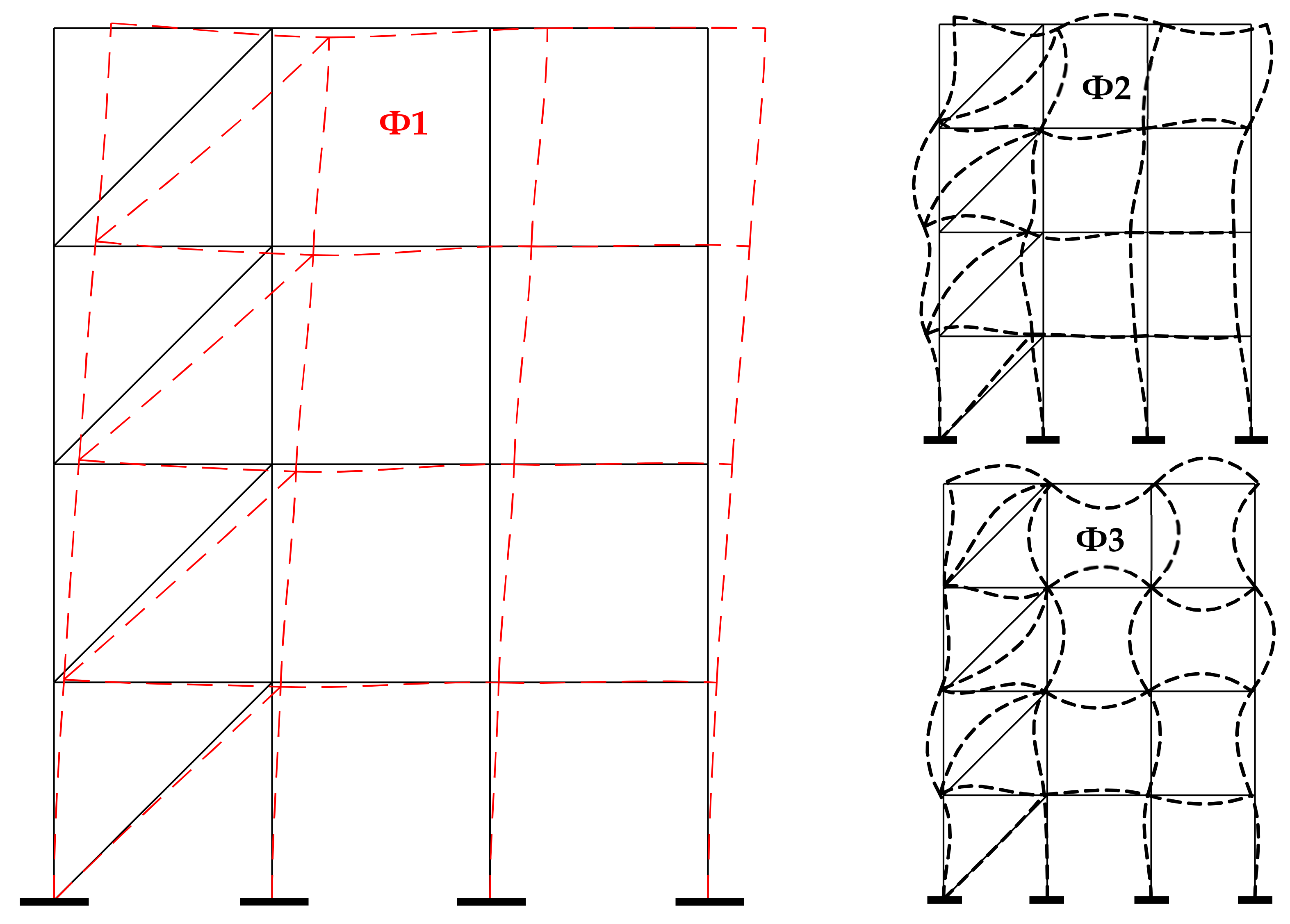
Next, the calculation is repeated with diagonal bracing added to each floor, restricting horizontal displacement and minimizing the side-sway frame effect as shown in Figure 9. The statistics of the corrected calculation are shown in Table 7, modelling bars with one element. The relative error is reduced significantly in all modes except the third. Our distortion criterion detects the problem since all distortion factors lie above 100% by a very wide margin. As expected, the one-element discretization leads to large errors for a non-sway structure with highly localized vibration shapes from the second mode on.
According to our distortion criterion, we should subdivide the 7 distorted elements from mode 3 onwards. However, for easiness of implementation we only split the four diagonals and that was enough to reduce the error to very low values (see Table 8). We inspect the second and third mode with subdivided diagonals in Figure 10 and we can see that those modes are highly localized in the diagonal bars. We can interpret that the one-element correction does not decrease error well in Table 7 because it replaces the second and third mode with local vibrations inside the bars, which is easily detected by our distortion factor.
Therefore, whenever the local correction can produce an inner vibration softer than the coarse mesh mode, it will distort all the modes from that frequency onwards. That is one of the reasons why we chose a two element submodel instead of a four element one like in our previous buckling study [37] because this problem does not appear when only the lowest eigenvalue is required.
5.2. 3D Stand Structure
This test case taken from [8] and fully defined in [37] is shown in Figure 11. This is not a typical portal frame structure, which confirms the validity of our approach for generic structural types.
The first modal shape Ф1 (red dashed lines) is superimposed on the undeformed geometry (continuous black lines). The second shape is very similar to the first one (also a translation of the roof but in a perpendicular direction). The third and fourth shapes (Ф3 and Ф4) are shown on the right in smaller sizes.
Numerical results are shown in Table 9 with one element per member. A relative error decrease exceeding a factor of 11 is obtained in all cases. The single-element-per-member discretization is quite accurate except for the 4th mode, which shows a distortion factor slightly larger than 100% and should therefore be split in half. Modes 1 to 3 can be considered sway modes (two translations and one rotation of the roof), whereas mode 4 almost keeps the beam ends in their original positions.
5.3. 3D Building Structure
This test case taken from [37] is shown in Figure 12. The 1st and 12th modal shapes, (red dashed lines) are superimposed on the undeformed geometry (continuous black lines).
Numerical results are shown in Table 10 for the first 12 modes (the number of floor translational and rotational movements). Although the frame is unbraced and thus does not localize vibration shapes, leading to quite accurate results with a one-element calculation, the relative error is still reduced by a factor greater than 10.
Figure 13 displays the same calculation after adding diagonal bracing bars. These bars help keep the structure from swaying side to side horizontally.
Numerical results are shown in Table 11 with one element per member. The relative error is largely decreased by the correction except for the last four modes, when distortion factors reach high values. Errors are higher in this case because of the bracing preventing large amplitude sway modes.
Numerical results are shown in Table 12 with two elements per member, even though according to our criterion only 42 out of the 160 bars would need two elements. By applying the correction, we reduce the relative error to a very good level of just 0.06%. It is worth noting that a two-element model of the structure with our correction could be an interesting alternative because of the low errors and distortion factors of the elements, which would make further subdivision unnecessary.
After examining the results, we can conclude that our models achieve the same level of accuracy as Abaqus standard FEM models with twice as many bars (on the condition that distortion factors lie below 100%), therefore they can work with stiffness and mass matrices twice smaller. In addition, we have attained calculation times 15% smaller measuring the main components of required processing power, i.e., the whole frame eigenvalue problem and the local beam eigenvalue problems.
6. Discussion
The method by Xie and Steven [10] provides local natural frequency updates for single bars rather than local modal shape corrections, which leads to using a weighted criterion with a weaker physical foundation than Rayleigh’s quotient. In addition, structural members are discretized with four or five elements while in our case one or two (in a few bars) elements are needed.
The SPRD technique by Wiberg et al. [18] bears some similarities with our approach. It relies on a polynomial fitting to the existing mode at some superconvergent points while our procedure completely updates the mode at inner points without being constrained by the coarse calculation on the inside. Plus, the whole structure rather than a single element and its neighboring patch participates in the adjustment by means of the coarse modal amplitude η. It can also be noted that SPR techniques use an external patch of elements while our method relies on an inner set of refined elements.
Gradient smoothing methods such as [19] also rely on neighboring elements to improve the quality of the solution but they do it before solving the system of equations of the whole structure, thereby increasing connectivity and the enhanced element matrix computation time. In addition, there is no straightforward way of applying the smoothing concept to beam elements of different sections and orientations sharing a node.
Modified stiffness and mass matrices [29], while improving the accuracy of dynamic analysis, are limited by the fact that they do not depend on the natural frequency being studied (like in the case of dynamic stiffness methods) or on the actual modal shape, as happens in our method.
Higher-order finite elements [31,32,33,34] provide better accuracy but are more complex to implement, have to solve larger systems of equations and lead to worse conditioned matrices. In contrast, our method works well with the standard finite element method and could work with higher-order finite elements as well to improve their accuracy. As for thin-walled beams [36], they require higher-order models in order to represent complex deformation patterns, but they are fully compatible with our correction algorithm.
The hierarchical FEM [23,24,25] relies on error estimators to refine the structural mesh and improve accuracy. In contrast, our correction does not need a full reanalysis to increase precision but an array of concurrent element-centered corrections. If necessary, the distortion factor indicates what bars require two elements instead of one. Like the higher-order elements discussed above, hierarchical elements of higher order can be used for the corrections instead of our two-subelement set.
As mentioned in the introduction, the authors recently wrote a closely related paper [37] about calculating the critical buckling loads of structural frames using one element per member. For this purpose, a local correction procedure was applied using four subelements. This latest work presents some fundamental differences. First, preventing structural buckling requires knowing just the lowest critical load, but in order to model structural dynamics accurately, multiple natural frequencies are needed. Second, the interplay between multiple frequencies coupled with the limited accuracy of individual elements makes it necessary to use two subelements instead of four. Third, because of the smaller number of subelements involved in the local corrections, some members have to be split into half beams according to a novel element distortion criterion which measures the relative change in kinetic and elastic energy caused by the correction of modal shapes.
As far as the efficiency of our method is concerned, most of what was stated in [37] remains applicable: the algorithm’s greatest source of efficiency comes from its fully parallelizable nature and the local eigenvalue problems can be solved with minimal computational resources by the power method. In addition, after shrinking the submodel to two elements, all the matrices that appear in the local eigenvalue problem can be easily programmed with scalar operators and functions, thereby reducing the cost to solving the eigenvalue problem.
Our technique can be applied to enhance the standard FEM analysis of any structure made up of beam/column elements. The structure could also contain shell, plate or lumped elements but the gain in accuracy would only occur for the bar elements. Our approach can be used to calculate natural frequencies with errors acceptable in engineering (below 1%) using one or two elements per member or to increase the accuracy of a calculation with any number of elements per member. Therefore, our approach offers the potential for a reduction in memory requirements and calculation speed when compared with the standard FEM at the cost of some additional coding. In order to fully exploit the advantages of the algorithm, it is advisable to distribute the correction calculations to the GPU.
Concerning future research developments based on the present work, we have selected a few areas of interest. First, there is always a significant discrepancy between numerical vibrational properties and experimental measurements [39,40] because of approximate modelling, nonlinearities, temperature effects, etc., which could be addressed advantageously with the proposed numerical technique or an enhanced version of it. Likewise, in the field of health structural monitoring, there is also the need to deal with discrepancies caused by structural failure or deterioration, and to diagnose their nature and location [41,42]. However, the present study is only concerned with numerical efficiency and has no direct application in these areas in its present form.
7. Conclusions
A new method for improving the accuracy of the standard FEM natural frequency calculation of structural frames made up of beam/column elements has been presented. The algorithms are based on previous work by the authors on structural frame buckling, but significant novel modifications have been made to improve efficiency and ease implementation, and to account for the challenges of calculating several eigenvalues instead of the lowest one. The fully parallel nature of the method makes it very convenient to take advantage of the current trend towards GPU-based architectures. For this purpose, the main calculation cost driver is a small individual nodal centered eigenvalue problem solvable with a few power iterations.
Structural members are modelled with one or two elements following a novel subdivision criterion based on the degree of distortion caused by the correction of the original modal shape. As a result, enough accuracy for engineering applications is achieved with a modest increase in computation time and storage requirements. The approach is very flexible and can accommodate different beam types, higher-order models and finer meshes and target precision levels, even though it has been demonstrated with simple cubic elements. Algorithm inputs are readily available data on FEM codes such as frame and element stiffness and mass matrices, rotations and modal shapes that can be processed with scalar functions and operators before the local eigensolver correction step.
Author Contributions
Conceptualization, J.U.: methodology, J.U.; software, J.U.; validation, J.U. and I.G.; writing, J.U. and I.G. All authors have read and agreed to the published version of the manuscript.
Funding
This research received no external funding.
Data Availability Statement
The original contributions presented in the study are included in the article. Further inquiries can be directed to the corresponding author.
Conflicts of Interest
The authors declare no conflict of interest.
References
- Chopra, A.K. Dynamics of Structures: Theory and Applications to Earthquake Engineering, 6th ed.; Pearson: London, UK, 2023. [Google Scholar]
- Spanish Structural Code (Código Estructural); Spanish Ministry of Transport, Mobility and the Urban Agenda (Ministerio de Transportes, Movilidad y Agenda Urbana): Madrid, Spain, 2021.
- EN1993-1-1; Eurocode 3: Design of Steel Structures. European Committee for Standardization: Brussels, Belgium, 2005.
- Staff, American Society of Civil Engineers (ASCE). Minimum Design Loads for Buildings and Other Structures, 3rd ed.; American Society of Civil Engineers: Reston, VA, USA, 2013. [Google Scholar]
- Biswas, P.; Peronto, J. Design and Performance of Tall Buildings for Wind, 1st ed.; American Society of Civil Engineers (ASCE): Reston, VA, USA, 2020. [Google Scholar]
- Petyt, M. Introduction to Finite Element Vibration Analysis, 2nd ed.; Cambridge University Press: Cambridge, UK, 2015. [Google Scholar]
- Zienkiewicz, O.C.; Taylor, R.L.; Zhu, J.Z. The Finite Element Method: Its Basis and Fundamentals; Butterworth-Heinemann: Cambridge, UK, 2013; Volume 3. [Google Scholar]
- Xie, Y.M.; Steven, G.P. Improving finite element predictions of buckling loads of beams and frames. Comput. Struct. 1994, 52, 381–385. [Google Scholar] [CrossRef]
- Mackie, R.I. Improving finite element predictions of modes of vibration. Int. J. Numer. Methods Eng. 1992, 33, 333–344. [Google Scholar] [CrossRef]
- Xie, Y.M.; Steven, G.P. Explicit formulas for correcting finite-element predictions of natural frequencies. Commun. Numer. Methods Eng. 1993, 9, 671–680. [Google Scholar] [CrossRef]
- Babuška, I.; Rheinboldt, W.C. A-posteriori error estimates for the finite element method. Int. J. Numer. Methods Eng. 1978, 12, 1597–1615. [Google Scholar] [CrossRef]
- Babuška, I. Accuracy Estimates and Adaptive Refinements in Finite Element Computations; Wiley: Chichester, UK, 1986. [Google Scholar]
- Zienkiewicz, O.C.; Zhu, J.Z. The superconvergent patch recovery (SPR) and adaptive finite element refinement. Comput. Methods Appl. Mech. Eng. 1992, 101, 207–224. [Google Scholar] [CrossRef]
- Boroomand, B.; Zienkiewicz, O.C. Recovery by equilibrium in patches (REP). Int. J. Numer. Methods Eng. 1997, 40, 137–164. [Google Scholar] [CrossRef]
- Sun, H.; Yuan, S. An improved local error estimate in adaptive finite element analysis based on element energy projection technique. Eng. Comput. 2023, 40, 246–264. [Google Scholar] [CrossRef]
- Wiberg, N.-E.; Abdulwahab, F.; Ziukas, S. Improved element stresses for node and element patches using superconvergent patch recovery. Commun. Numer. Methods Eng. 1995, 11, 619–627. [Google Scholar] [CrossRef]
- Wiberg, N.; Abdulwahab, F. Patch recovery based on superconvergent derivatives and equilibrium. Int. J. Numer. Methods Eng. 1993, 36, 2703–2724. [Google Scholar] [CrossRef]
- Wiberg, N.; Bausys, R.; Hager, P. Improved eigenfrequencies and eigenmodes in free vibration analysis. Comput. Struct. 1999, 73, 79–89. [Google Scholar] [CrossRef]
- Liu, G.R. A generalized gradient smoothing technique and the smoothed bilinear form for Galerkin formulation of a wide class of computational methods. Int. J. Comput. Methods 2008, 5, 199–236. [Google Scholar] [CrossRef]
- Liu, G.R. On G space theory. Int. J. Comput. Methods 2009, 6, 257–289. [Google Scholar] [CrossRef]
- Liu, G.R.; Nguyen-Thoi, T.; Nguyen-Xuan, H.; Lam, K.Y. A node-based smoothed finite element method (NS-FEM) for upper bound solutions to solid mechanics problems. Comput. Struct. 2009, 87, 14–26. [Google Scholar] [CrossRef]
- Liu, G.R.; Nguyen-Thoi, T.; Lam, K.Y. An edge-based smoothed finite element method (ES-FEM) for static, free and forced vibration analyses of solids. J. Sound Vib. 2009, 320, 1100–1130. [Google Scholar] [CrossRef]
- Zienkiewicz, O.C.; De, S.R.; Gago, J.P.; Kelly, D.W. The hierarchical concept in finite element analysis. Comput. Struct. 1983, 16, 53–65. [Google Scholar] [CrossRef]
- Ganesan, N.; Engels, R.C. Hierarchical Bernoulli-Euler beam finite elements. Comput. Struct. 1992, 43, 297–304. [Google Scholar] [CrossRef]
- Tai, C.-Y.; Chan, Y.J. A hierarchic high-order Timoshenko beam finite element. Comput. Struct. 2016, 165, 48–58. [Google Scholar] [CrossRef]
- Hui, Y.; Giunta, G.; Belouettar, S.; Huang, Q.; Hu, H.; Carrera, E. A free vibration analysis of three-dimensional sandwich beams using hierarchical one-dimensional finite elements. Compos. Part B Eng. 2017, 110, 7–19. [Google Scholar] [CrossRef]
- Fried, I.; Chavez, M. Superaccurate finite element eigenvalue computation. J. Sound Vib. 2004, 275, 415–422. [Google Scholar] [CrossRef]
- Fried, I.; Leong, K. Superaccurate finite element eigenvalues via a Rayleigh quotient correction. J. Sound Vib. 2005, 288, 375–386. [Google Scholar] [CrossRef]
- Li, E.; He, Z.C. Development of a perfect match system in the improvement of eigenfrequencies of free vibration. Appl. Math. Model. 2017, 44, 614–639. [Google Scholar] [CrossRef]
- Guddati, M.N.; Yue, B. Modified integration rules for reducing dispersion error in finite element methods. Comput. Methods Appl. Mech. Eng. 2004, 193, 275–287. [Google Scholar] [CrossRef]
- Shang, H.Y.; Machado, R.D.; Abdalla Filho, J.E. Dynamic analysis of Euler–Bernoulli beam problems using the Generalized Finite Element Method. Comput. Struct. 2016, 173, 109–122. [Google Scholar] [CrossRef]
- Hsu, Y.S. Enriched finite element methods for Timoshenko beam free vibration analysis. Appl. Math. Model. 2016, 40, 7012–7033. [Google Scholar]
- Cornaggia, R.; Darrigrand, E.; Le Marrec, L.; Mahé, F. Enriched finite elements and local rescaling for vibrations of axially inhomogeneous Timoshenko beams. J. Sound Vib. 2020, 474, 115228. [Google Scholar] [CrossRef]
- Necib, B.; Sun, C.T. Analysis of truss beams using a high order Timoshenko beam finite element. J. Sound Vib. 1989, 130, 149–159. [Google Scholar] [CrossRef]
- Wang, T.; Mikkola, A.; Matikainen, M.K. An Overview of Higher-Order Beam Elements Based on the Absolute Nodal Coordinate Formulation. J. Comput. Nonlinear Dynam. 2022, 17, 091001. [Google Scholar] [CrossRef]
- Nguyen, T.; Nguyen, N.; Lee, J.; Nguyen, Q. Vibration analysis of thin-walled functionally graded sandwich beams with non-uniform polygonal cross-sections. Compos. Struct. 2021, 278, 114723. [Google Scholar] [CrossRef]
- Urruzola, J.; Garmendia, I. Calculation of Linear Buckling Load for Frames Modeled with One-Finite-Element Beams and Columns. Computation 2023, 11, 109. [Google Scholar] [CrossRef]
- Meirovitch, L. Fundamentals of Vibrations; McGraw-Hill: New York, NY, USA, 2001. [Google Scholar]
- Luo, J.; Huang, M.; Lei, Y. Temperature Effect on Vibration Properties and Vibration-Based Damage Identification of Bridge Structures: A Literature Review. Buildings 2022, 12, 1209. [Google Scholar] [CrossRef]
- Huang, M.; Zhang, J.; Hu, J.; Ye, Z.; Deng, Z.; Wan, N. Nonlinear modeling of temperature-induced bearing displacement of long-span single-pier rigid frame bridge based on DCNN-LSTM. Case Stud. Therm. Eng. 2024, 53, 103897. [Google Scholar] [CrossRef]
- Deng, Z.; Huang, M.; Wan, N.; Zhang, J. The Current Development of Structural Health Monitoring for Bridges: A Review. Buildings 2023, 13, 1360. [Google Scholar] [CrossRef]
- Huang, M.; Ling, Z.; Sun, C.; Lei, Y.; Xiang, C.; Wan, Z.; Gu, J. Two-stage damage identification for bridge bearings based on sailfish optimization and element relative modal strain energy. Struct. Eng. Mech. Int. J. 2023, 86, 715–730. [Google Scholar]
Figure 1.
Five fundamental beam vibration cases.

Figure 2.
Bar element “global” displacement (from 1–3 to 1′–3′).

Figure 3.
Element incremental local displacements (from 1–3 to 1′–3′).

Figure 4.
Refined element total displacements (global from 1–3 to 1′3′ and local from 1’–3’ to 1”–3”).
Figure 4.
Refined element total displacements (global from 1–3 to 1′3′ and local from 1’–3’ to 1”–3”).

Figure 5.
Locally corrected PP2 modal shape using one element and two subelements.

Figure 6.
PP2 modal shape using two elements after local correction.

Figure 7.
Structural discretization used to correct the upper part of two-element PP2 modal shape.

Figure 8.
2D sway portal: first three modal shapes with one element per member.

Figure 9.
2D framed portal frame: first three modal shapes with one element per member.

Figure 10.
2D braced portal frame: 2nd and 3rd modal shapes with one element per member except diagonals (two).
Figure 10.
2D braced portal frame: 2nd and 3rd modal shapes with one element per member except diagonals (two).

Figure 11.
3D stand frame modal shapes 1, 3 and 4.

Figure 12.
3D sway 160-bar building structure 1st (left) and 12th (right) modal shapes.

Figure 13.
3D braced building structure 1st and 12th modal shapes with one element per member.


Table 1.
Relative error 1 in natural frequency computation for some fundamental cases.
| Nel 2 | CC | CP | PP | CF | PP2 |
|---|---|---|---|---|---|
| 1 | - | 32.92% | 10.99% | 0.48% | 27.14% |
| 2 | 1.62% | 0.93% | 0.39% | 0.05% | 10.98% |
| 3 | 0.41% | 0.20% | 0.08% | 0.01% | 1.17% |
| 4 | 0.13% | 0.06% | 0.03% | 0.00% | 0.38% |
1 Relative error refers to “nearly exact” values calculated with Abaqus and Nel = 10. 2 Nel: number of elements in the discretization.
Table 2.
Relative error in corrected natural frequency calculation (Nel = 1).
| Nel | CC | CP | PP | CF | PP2 |
|---|---|---|---|---|---|
| 1 | 1.61% | 0.93% | 0.39% | 0.05% | 42.42% |
Table 3.
Distortion factor (maximum percentage change in V or T) after correction (Nel = 1).
| Nel | CC | CP | PP | CF | PP2 |
|---|---|---|---|---|---|
| 1 | -% | 211.33% | 49.66% | 1.73% | 1.4 × 1029% |
Table 4.
Relative error in corrected natural frequency calculation with one and two elements per member.
Table 4.
Relative error in corrected natural frequency calculation with one and two elements per member.
| Nel | CC | CP | PP | CF | PP2 |
|---|---|---|---|---|---|
| 1 | 1.61% | 0.93% | 0.39% | 0.05% | 42.42% |
| 2 | 0.13% | 0.06% | 0.03% | 0.00% | 0.47% |
Table 5.
Maximum percentage change in Ve or Te with one and two elements per member after applying the proposed correction.
Table 5.
Maximum percentage change in Ve or Te with one and two elements per member after applying the proposed correction.
| Nel | CC | CP | PP | CF | PP2 |
|---|---|---|---|---|---|
| 1 | -% | 211.33% | 49.66% | 1.73% | 1.4 × 1029% |
| 2 | 6.28% | 2.57% | 1.49% | 0.09% | 55.81% |
Table 6.
Corrected calculation statistics (2D sway portal frame with 1 element/member).
| Mode # | Exact 1 ω (rad/s) | 1-Elem. 2 ω (rad/s) | Relative 3 Error (%) | Corrected ω (rad/s) 4 | Relative 5 Error (%) | Distortion Factor γ (%) | Distorted Elements # |
|---|---|---|---|---|---|---|---|
| 1 | 34.88 | 34.89 | 0.02 | 34.88 | 0.00 | 1.14 | 0 |
| 2 | 110.12 | 110.28 | 0.14 | 110.13 | 0.01 | 6.11 | 0 |
| 3 | 195.67 | 196.28 | 0.31 | 195.73 | 0.03 | 4.27 | 0 |
| 4 | 277.60 | 278.38 | 0.28 | 277.75 | 0.05 | 6.46 | 0 |
1 “Exact” value of ω calculated with Abaqus and Nel = 10. 2 Value of ω calculated with Abaqus and Nel = 1. 3 Relative error of the 1-element calculation 4 Value of ω after applying our correction to the 1-element value. 5 Relative error of the corrected value.
Table 7.
Corrected calculation statistics (2D braced portal frame with 1 element/member).
| Mode # | Exact ω (rad/s) | 1-Elem. Ω (rad/s) | Relative Error (%) | Corrected ω (rad/s) | Relative Error (%) | Distortion Factor γ (%) | Distorted Elements # |
|---|---|---|---|---|---|---|---|
| 1 | 161.75 | 162.68 | 0.57 | 161.81 | 0.04 | 125 | 1 |
| 2 | 438.18 | 551.89 | 25.95 | 471.27 | 7.55 | 2854 | 7 |
| 3 | 447.47 | 579.72 | 29.56 | 575.00 | 28.50 | 1.3 × 10⁸ | 4 |
| 4 | 473.87 | 631.82 | 33.33 | 516.46 | 8.99 | 14,137 | 5 |
Table 8.
Corrected calculation statistics (2D braced portal frame with 2 elems./member diagonals).
| Mode # | Exact ω (rad/s) | 1/2-Elem. ω (rad/s) | Relative Error | Corrected ω (rad/s) | Relat. Error | Distortion Factor γ | Distorted Elements # |
|---|---|---|---|---|---|---|---|
| 1 | 161.75 | 162.25 | 0.31% | 161.78 | 0.02% | 122% | 1 |
| 2 | 438.18 | 446.60 | 1.92% | 438.83 | 0.15% | 145% | 2 |
| 3 | 447.47 | 456.15 | 1.94% | 448.13 | 0.15% | 63% | 0 |
| 4 | 473.87 | 482.68 | 1.86% | 474.53 | 0.14% | 364% | 1 |
Table 9.
Corrected calculation statistics (3D stand with 1 elem./member).
| Mode # | Exact 1 ω (rad/s) | 1-Elem. ω (rad/s) | Relative Error (%) | Corrected ω (rad/s) | Relative Error (%) | Distortion Factor γ (%) | Distorted Elements # |
|---|---|---|---|---|---|---|---|
| 1 | 97.41 | 97.59 | 0.19 | 97.42 | 0.01 | 3.48 | 0 |
| 2 | 97.41 | 97.59 | 0.19 | 97.42 | 0.01 | 3.52 | 0 |
| 3 | 140.11 | 140.45 | 0.24 | 140.14 | 0.02 | 6.40 | 0 |
| 4 | 580.82 | 672.56 | 15.79 | 583.93 | 1.38 | 101.45 | 4 |
1 “Exact” value calculated with Abaqus and Nel = 10.
Table 10.
Corrected calculation statistics (3D sway building structure with 1 elem./member).
| Mode # | Exact ω (rad/s) | 1-Elem. ω (rad/s) | Relative Error (%) | Corrected ω (rad/s) | Relative Error (%) | Distortion Factor γ (%) | Distorted Elements # |
|---|---|---|---|---|---|---|---|
| 1 | 28.51 | 28.51 | 0.01 | 28.51 | 0.00 | 8.20 | 0 |
| 2 | 28.51 | 28.51 | 0.01 | 28.51 | 0.00 | 8.20 | 0 |
| 3 | 31.81 | 31.82 | 0.02 | 31.81 | 0.00 | 2.01 | 0 |
| 4 | 89.08 | 89.20 | 0.14 | 89.09 | 0.01 | 67.43 | 0 |
| 5 | 89.08 | 89.20 | 0.14 | 89.09 | 0.01 | 64.86 | 0 |
| 6 | 91.72 | 91.85 | 0.14 | 91.73 | 0.01 | 50.67 | 0 |
| 7 | 98.90 | 99.05 | 0.15 | 98.91 | 0.01 | 4.79 | 0 |
| 8 | 129.38 | 129.72 | 0.26 | 129.41 | 0.02 | 11.55 | 0 |
| 9 | 137.88 | 138.27 | 0.29 | 137.91 | 0.02 | 56.25 | 0 |
| 10 | 137.88 | 138.27 | 0.29 | 137.91 | 0.02 | 55.71 | 0 |
| 11 | 155.42 | 156.00 | 0.38 | 155.46 | 0.03 | 189.21 | 4 |
| 12 | 155.42 | 156.00 | 0.38 | 155.46 | 0.03 | 99.61 | 0 |
Table 11.
Corrected calculation statistics (3D braced building structure with 1 elem./member).
| Mode # | Exact ω (rad/s) | 1-Elem. ω (rad/s) | Relative Error (%) | Corrected ω (rad/s) | Relative Error (%) | Distortion Factor γ (%) | Distorted Elements # |
|---|---|---|---|---|---|---|---|
| 1 | 124.49 | 125.17 | 0.54 | 124.54 | 0.04 | 47.18 | 0 |
| 2 | 126.75 | 127.42 | 0.53 | 126.79 | 0.04 | 59.22 | 0 |
| 3 | 146.27 | 147.08 | 0.55 | 146.33 | 0.04 | 80.42 | 0 |
| 4 | 151.65 | 152.58 | 0.61 | 151.71 | 0.04 | 76.67 | 0 |
| 5 | 184.03 | 185.26 | 0.67 | 184.13 | 0.06 | 182.87 | 1 |
| 6 | 212.50 | 214.77 | 1.07 | 212.67 | 0.08 | 185.24 | 6 |
| 7 | 245.42 | 248.36 | 1.20 | 245.69 | 0.11 | 273.57 | 13 |
| 8 | 276.69 | 281.67 | 1.80 | 277.20 | 0.18 | 729.64 | 18 |
| 9 | 366.95 | 402.78 | 9.77 | 372.53 | 1.52 | 1907.05 | 41 |
| 10 | 384.71 | 434.85 | 13.03 | 396.66 | 3.11 | 2970.10 | 51 |
| 11 | 392.67 | 454.37 | 15.72 | 423.86 | 7.94 | 1200.18 | 35 |
| 12 | 403.95 | 467.65 | 15.77 | 433.75 | 7.38 | 2018.34 | 42 |
Table 12.
Corrected calculation statistics (3D braced building structure with 2 elems./member).
| Mode # | Exact ω (rad/s) | 2-Elem. ω (rad/s) | Relative Error (%) | Corrected ω (rad/s) | Relative Error (%) | Distortion Factor γ (%) | Distorted Elements # |
|---|---|---|---|---|---|---|---|
| 1 | 124.49 | 124.54 | 0.03 | 124.50 | 0.00 | 2.35 | 0 |
| 2 | 126.75 | 126.79 | 0.03 | 126.75 | 0.00 | 4.65 | 0 |
| 3 | 146.27 | 146.33 | 0.04 | 146.28 | 0.00 | 3.94 | 0 |
| 4 | 151.65 | 151.71 | 0.04 | 151.66 | 0.00 | 4.33 | 0 |
| 5 | 184.03 | 184.13 | 0.05 | 184.04 | 0.00 | 6.87 | 0 |
| 6 | 212.50 | 212.66 | 0.08 | 212.52 | 0.01 | 4.66 | 0 |
| 7 | 245.42 | 245.67 | 0.10 | 245.44 | 0.01 | 7.20 | 0 |
| 8 | 276.69 | 277.13 | 0.16 | 276.73 | 0.01 | 17.03 | 0 |
| 9 | 366.95 | 368.89 | 0.53 | 367.08 | 0.04 | 9.62 | 0 |
| 10 | 384.71 | 387.27 | 0.67 | 384.89 | 0.05 | 16.12 | 0 |
| 11 | 392.67 | 395.59 | 0.74 | 392.87 | 0.05 | 3.82 | 0 |
| 12 | 403.95 | 407.28 | 0.82 | 404.18 | 0.06 | 4.83 | 0 |
Disclaimer/Publisher’s Note: The statements, opinions and data contained in all publications are solely those of the individual author(s) and contributor(s) and not of MDPI and/or the editor(s). MDPI and/or the editor(s) disclaim responsibility for any injury to people or property resulting from any ideas, methods, instructions or products referred to in the content. |
© 2024 by the authors. Licensee MDPI, Basel, Switzerland. This article is an open access article distributed under the terms and conditions of the Creative Commons Attribution (CC BY) license (https://creativecommons.org/licenses/by/4.0/).
Share and Cite
MDPI and ACS Style
Urruzola, J.; Garmendia, I. Improved FEM Natural Frequency Calculation for Structural Frames by Local Correction Procedure. Buildings 2024, 14, 1195. https://doi.org/10.3390/buildings14051195
AMA Style
Urruzola J, Garmendia I. Improved FEM Natural Frequency Calculation for Structural Frames by Local Correction Procedure. Buildings. 2024; 14(5):1195. https://doi.org/10.3390/buildings14051195
Chicago/Turabian StyleUrruzola, Javier, and Iñaki Garmendia. 2024. "Improved FEM Natural Frequency Calculation for Structural Frames by Local Correction Procedure" Buildings 14, no. 5: 1195. https://doi.org/10.3390/buildings14051195
Note that from the first issue of 2016, this journal uses article numbers instead of page numbers. See further details here.