Study on the Ionic Transport Properties of 3D Printed Concrete

1
School of Engineering, Architecture and the Environment, Hubei University of Technology, Wuhan 430086, China
2
Key Laboratory of Intelligent Health Perception and Ecological Restoration of Rivers and Lakes, Ministry of Education, Hubei University of Technology, Wuhan 430086, China
*
Author to whom correspondence should be addressed.
Buildings 2024, 14(5), 1216; https://doi.org/10.3390/buildings14051216
Submission received: 25 March 2024
/
Revised: 20 April 2024
/
Accepted: 21 April 2024
/
Published: 24 April 2024
(This article belongs to the Section Building Materials, and Repair & Renovation)
Abstract
:Three-dimensional printed concrete (3DPC) is an anisotropic heterogeneous material composed of a concrete matrix and the interfaces between layers and filaments that form during printing. The overall ion transport properties can be characterized by the equivalent diffusion coefficient. This paper first establishes a theoretical model to calculate the equivalent diffusion coefficient of 3DPC. Verification through numerical calculations shows that this theoretical model is highly precise. Based on this, the model was used to analyze the effects of dimensionless interface parameters on the equivalent diffusion coefficients in different directions of 3DPC. Finally, the dynamic ionic transport properties of 3DPC were investigated through finite element numerical simulation. The results of the dynamic study indicate that interfaces have a significant impact on the ion distribution and its evolution within 3DPC. The product of the interface diffusion coefficient and interface size can represent the ionic transport capacity of an interface. The stronger the ionic transport capacity of an interface, the higher the ion concentration at that interface. Due to the “drainage” effect of lateral interfaces, the ion concentration in the middle of 3DPC with a smaller equivalent diffusion coefficient is higher than that in 3DPC with a larger equivalent diffusion coefficient.
1. Introduction
As one of the advanced additive manufacturing (AM) technologies, 3D printed concrete (3DPC) integrates numerous cutting-edge scientific technologies, including digital design and material engineering [1,2]. Recently, 3DPC has garnered significant attention for its ability to eliminate the need for concrete molds, thus enabling the construction of buildings with more complex geometries and higher precision [3,4]. As an additive manufacturing technology, 3DPC precisely controls the material, thereby reducing construction costs and environmental pollution [5]. Its advantages also include reduced manual labor, lowering the risk of accidents, and offering the flexibility to adjust building structures according to designers’ requirements. This flexibility helps to accommodate various construction, size, and functional requirements and saves construction time [6].
Despite its numerous advantages, 3DPC faces several challenges that need addressing. Due to the absence of molds, exposure to environmental conditions (wind, rain, temperature, carbon dioxide, chemical ions, etc.) may cause greater deformation of the concrete. This deformation can lead to the formation of microcracks or an increase in porosity, thus creating preferential pathways for the transport of harmful substances [7,8,9]. Furthermore, the layer-by-layer construction inherent to 3DPC introduces significant porosity between layers and filaments. These pores tend to align, creating directional channels that accelerate the corrosion process and adversely affect the structural integrity and durability of 3DPC [10]. Consequently, reinforcing and minimizing the vulnerabilities at the interfaces between layers and filaments during printing is of utmost importance [11].
Previous research has indicated that chloride penetration, along with the initiation and propagation of corrosion on reinforcement, are among the primary reasons for reducing concrete durability in reinforced concrete. With the emergence of 3DPC technology, researchers have attempted to incorporate steel reinforcement to address its inherent weakness in bending resistance. This includes the design of steel reinforcement printing devices, synchronous insertion of rebar [12,13], interlayer reinforcement mesh embedding [14], and post-printing reinforced concrete casting [15,16]. Consequently, the study of chloride ion diffusion in 3DPC has become increasingly crucial.
Researchers have already investigated the diffusivity of chloride ions in 3DPC. For instance, Xu et al. [7] examined the impact of printing time intervals on the resistance of interlayer interfaces in 3DPC to chloride ion penetration. Surehali et al. [6] investigated how the height and width of each printed layer, the printing speed, and the quality of interlayer and inter-filament interfaces affect the directionality of moisture and harmful ion transport. Their research involved analyzing the porosity and conductivity of the microstructure of 3DPC samples to understand the effect of anisotropy on transport properties. Malan et al. [17] studied the durability of interlayer interfaces in 3DPC, comparing it with cast concrete of the same material composition. Their findings indicated that cast samples outperformed 3D printed samples in terms of durability, underscoring the importance of improving the interface properties of 3DPC.
However, current research on the ion transport properties and durability of 3DPC primarily relies on experiments, with few studies utilizing numerical simulations. Given the complex structure of 3DPC and the variability of environmental factors, conducting experimental research becomes complicated. Building on 3DPC ion diffusion experiments, this study proposes an algorithm based on Fick’s laws of diffusion to calculate the thickness and diffusion coefficients of the interlayer and inter-filament interfaces in 3DPC. The accuracy of the calculations was verified by comparing theoretical calculations with finite element simulation results. This method allows for a more precise determination of the thickness diffusion coefficients of the interlayer and inter-filament interfaces and the establishment of a numerical model for 3DPC. Through simulation calculations, the performance of 3DPC can be assessed more conveniently and quickly, with its durability predicted.
2. Equivalent Diffusion Coefficient Calculation Model
Moradllo [18] experimentally validated that the process of ion penetration in concrete adheres to Fick’s laws of diffusion, described by the following equations:
where represents the ion concentration within the concrete, denotes the erosion time, is the ion diffusion flux, is the diffusion coefficient of the concrete, and indicates the diffusion distance.
3DPC can be viewed as a biphasic system composed of the matrix and weak interface layers. Its diffusion performance depends on both the inherent diffusion properties of the concrete matrix and the diffusion properties and distribution of the weak interfaces [19]. An equivalent diffusion coefficient can characterize the overall diffusion performance of 3DPC. Constructed as a regular biphasic system through a layer-by-layer printing mechanism, 3DPC allows for the derivation of calculation formulas for the equivalent diffusion coefficients in different directions using Fick’s laws, which is suitable for such a physically simple, anisotropic heterogeneous material.
2.1. Parallel Model and Series Model
The analysis begins by examining the equivalent diffusion coefficient of a biphasic system under parallel and series configurations. For generality, consider a regular biphasic system composed of three layers, simplified as a planar problem, as illustrated in Figure 1. The total thickness and width of the system are denoted by and , respectively, with each layer’s thickness represented by (), the matrix diffusion coefficient represented by , and the inclusion phase diffusion coefficient represented by .
If ions diffuse in the y-direction, the biphasic system can be considered a parallel model. Assuming the ion concentrations at the left and right boundaries are and , respectively, and that there is no flux at the top and bottom boundaries, the equivalent diffusion coefficient in the y-direction can be derived under these conditions. The total flux across the right boundary is given as follows:
where represents the average flux across the right boundary, with , , and being the fluxes through the upper matrix layer, interface layer, and lower matrix layer, respectively. According to Fick’s first law, as follows:
Bringing Equation (3) into Equation (2) simplifies it, as follows:
where , represents the volume fraction of the inclusion phase. Equation (4) is the formula for the equivalent diffusion coefficient of the biphasic system in the case of parallel connection.
If ions diffuse in the z-direction, the biphasic system can be considered a serial model. Assuming the ion concentrations at the upper and lower boundaries are and , respectively, with no flux at the left and right boundaries, and the ion concentrations on the upper and lower sides of the middle layer are and , respectively, the equivalent diffusion coefficient in the z-direction can be derived under these conditions. Since the flux across each cross-section perpendicular to the z-axis is equal, it follows that:
From (5), as follows:
For the biphasic system as a whole, the flux at the lower boundary can also be expressed as follows:
Equation (6) is simplified by adding Equation (7) to obtain the following:
Equation (8) is the formula for the equivalent diffusion coefficient of a biphasic system in the case of a series connection.
2.2. 3DPC Equivalent Diffusion Coefficient
The interlayer and inter-filament interfaces can be considered inclusion phases by deriving the equivalent diffusion coefficient of 3DPC based on the parallel and serial models of the biphasic system.
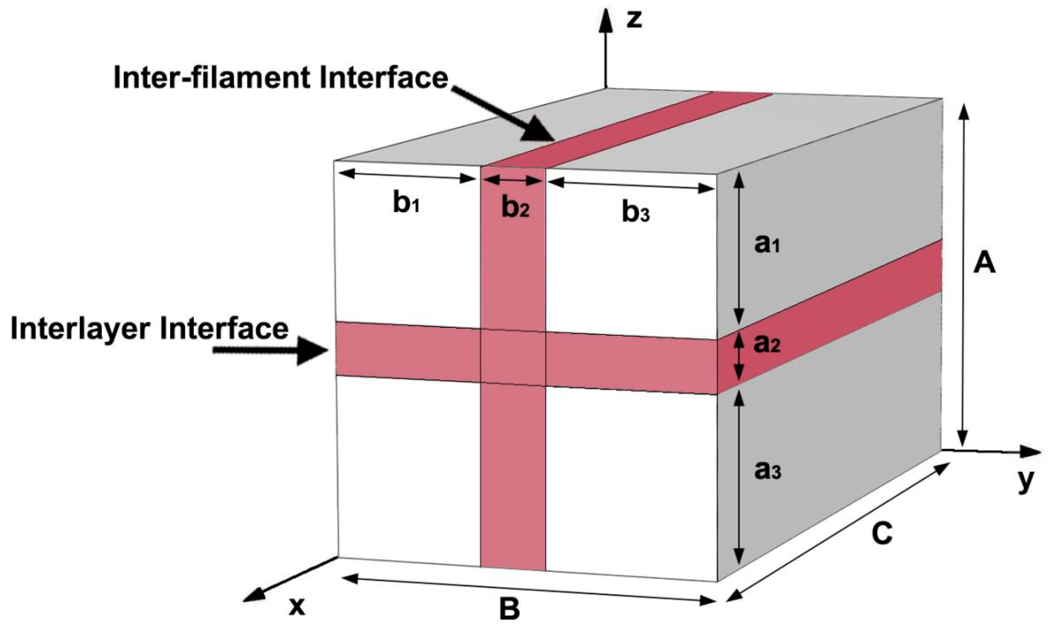
Without loss of generality, it is assumed that the 3DPC has only one interlayer interface and one inter-filament interface, as illustrated in the simplified model in Figure 2. The diffusion coefficients for the matrix, interlayer interface, and inter-filament interface are denoted as , , and , respectively. The total thickness, width, and length of the 3DPC are denoted as , , and , respectively. The thickness of the interlayer interface is , with the upper and lower matrix thicknesses as and , respectively. The width of the inter-filament interface is , with the left and right matrix widths as and , respectively.
When ions diffuse along the x-direction, the parallel model mentioned earlier can be applied to calculate the equivalent diffusion coefficient . Using Formula (4), we obtain the following:
where , represents the volume ratio of the interlayer interface, and , represents the volume ratio of the inter-filament interface.
When ions diffuse along the y-direction, the problem can be simplified to a planar issue, with the cross-section depicted in Figure 3. Utilizing the interlayer and inter-filament interfaces, 3DPC can be segmented into a grid of three rows by three columns, resulting in nine distinct sections, labeled 1 through 9. The diffusion coefficients for these sections are considered constant. The calculation of the equivalent diffusion coefficient can follow a methodology of “parallel-then-series” or “series-then-parallel”.
If the “parallel-first, series-second” approach is adopted, the equivalent diffusion coefficients for parts 1, 4, and 7 are first calculated using the parallel model.
where , represents the ratio of the interlayer interface thickness to the total thickness of the 3DPC. Similarly, the equivalent diffusion coefficients for parts 2, 5, and 8, and for parts 3, 6, and 9 can be calculated using the parallel model, yielding the following:
Then, using the series model to calculate the equivalent diffusion coefficients for the first, second, and third columns, we obtain the overall equivalent diffusion coefficient for the 3DPC under the “parallel-first, series-next” scenario, as follows:
where , represents the ratio of the width of the inter-filament interface to the total width of the 3DPC.
If adopting the “series-first, parallel-next” method, we first use the series model to calculate the equivalent diffusion coefficients for parts 1, 2, and 3; for parts 4, 5, and 6; and for parts 7, 8, and 9, resulting in the following:
Then, using the parallel model to calculate the equivalent diffusion coefficients for the first, second, and third rows, we obtain the overall equivalent diffusion coefficient for the 3DPC under the “series-first, parallel-next” scenario, as follows:
When ions diffuse in the z-direction, the method for calculating the equivalent diffusion coefficient is similar to that in the y-direction. If the “parallel-first, series-next” method is used, we obtain the following:
If the “series-first, parallel-next” method is adopted, we obtain the following:
2.3. Nondimensionalization of Equations
The equations were nondimensionalized to facilitate the discussion on the general trends in the variation of the effective diffusion coefficients for 3DPC.
Let υ denote the ratio of the total volume of all interfaces to the total volume of the 3DPC. Consequently, there exists a relationship among the interlayer interface ratio , the inter-filament interface ratio , and the volume ratio as follows:
When the υ is smaller, as follows:
Define the dimensionless parameter , , , , , and ; then, we can denote , , and as quaternions of , , , and . This allows for the simplification of Equations (9), (13), (17)–(19) to the following forms:
3. Finite Element Model
To verify the accuracy of the theoretical model described above, a 3DPC numerical model was established using the finite element software COMSOL 6.0 for steady-state ion transport analysis to calculate the equivalent diffusion coefficient of 3DPC. The simulation results were then compared with the theoretical calculations. The finite element model, as shown in Figure 4, applies different concentration loads ( and ) to two pairs of edges of the specimen, creating a concentration gradient in which ions diffuse from a high-concentration area to a low-concentration area, with the other two sides of the specimen being no-flux states. Accordingly, the specimen’s equivalent diffusion coefficient can be determined using the following formula, based on Fick’s laws of diffusion:
where and are the lengths of the specimen’s edges and is the diffusion flux at the specimen’s low concentration boundary.
To further investigate the dynamic ion transport properties of 3DPC, COMSOL was used to simulate the scenario of a 3DPC specimen immersed in a salt solution. The model, depicted in Figure 5, identifies the horizontal direction as the interlayer interface and the vertical direction as the inter-filament interface. The bottom surface of the specimen is immersed in a salt solution with a chloride ion concentration of , with no flux on the other surfaces. Chloride ions are transported upward from the bottom surface by diffusion, allowing for the analysis of differences in the dynamic ion transport properties of 3DPC with various structural parameters.
4. Analysis of Results
4.1. Theoretical Model Validation
Example 1, J. Van Der Putten et al. [20], investigated the impact of printing time intervals on the ion transport properties of 3DPC. In this experiment, the 3DPC consisted solely of interlayer interfaces. The matrix diffusion coefficient and the equivalent diffusion coefficient along the direction of the interlayer interface were measured. The related experimental data are listed in Table 1, and this case can be analyzed using a parallel model.
In this case, the interface thickness and the interface diffusion coefficient are unknown. It is assumed that varies from 0.1 mm to 1.5 mm (current research indicates that the interlayer thickness of 3DPC generally falls within the range of 0.1 mm to 1 mm [21,22,23,24,25]. To enhance the broad applicability of the numerical model in this study, a slightly higher value for interlayer thickness was chosen). Consequently, the interface diffusion coefficient can be calculated using the parallel model Equation (4), thereby establishing the relationship curve of as a function of , as illustrated in Figure 6.
To validate the accuracy of the parallel model’s theoretical equation, a 3DPC numerical model was developed using the COMSOL 6.0 software, based on the interface thickness and the structural parameters listed in Table 1. The interface diffusion coefficient , corresponding to , is input as the interface material parameter. The finite element method is then applied to simulate the steady-state ion transport within the 3DPC and to calculate the effective diffusion coefficient of the 3DPC. The simulated results are compared with the experimental values presented in Table 1, and these findings are also depicted in Figure 6.
As shown in Figure 6, the interfacial diffusion coefficient decreases with increasing interfacial thickness , but the rate of decrease gradually slows down. This phenomenon can be explained by Equation (4), in which is inversely proportional to . When the overall diffusion coefficient of the 3DPC remains constant, the diffusion coefficient at the interface decreases as the interfacial thickness increases. The simulated values of align perfectly with the experimental data, demonstrating the accuracy of the theoretical Equation (4) when applied to parallel configurations of 3DPC.
Example 2, S. Surehali et al. [6] investigated the relationship between the anisotropy of ion transport in 3DPC and variables such as layer height and interface type. Their experiment encompassed both interlayer and inter-filament interfaces within the 3DPC. It measured the matrix diffusion coefficient along with the effective diffusion coefficients in three different directions (, , and ) for the 3DPC. The relevant experimental data are presented in Table 2.
In this example, there are four unknown parameters, including the thickness of the interlayer interface and its diffusion coefficient , along with the width of the inter-filament interface and its diffusion coefficient . Assuming the range of is from 0.1 mm to 1.2 mm, the values for , , and can be calculated by solving a system of equations for , , and based on the theoretical model presented in Section 2.2. Depending on the combinations of series and parallel configurations, there are four different sets of equations. These are outlined in Table 3. The calculated values for , , and according to these four scenarios are listed in Table 4.
As can be observed from Table 4, for the same value of , there can be up to four different sets of solutions. When is small, scenarios 2 and 4 have no solution, while when is large, scenarios 1 and 4 have no solution. Relatively speaking, the solutions for scenarios 1 and 4 are similar, as are the solutions for scenarios 2 and 3. The variation patterns of the interlayer interface diffusion coefficient with interlayer interface thickness , as well as the inter-filament interface diffusion coefficient with inter-filament interface width , are shown in Figure 7. It can be seen from the figure that, regardless of the interface type, the variation trends of the interface diffusion coefficients calculated by different scenarios are essentially the same, approximately following an inverse proportional function relationship.
To verify the accuracy of the theoretical model and the solutions, a numerical model of the 3DPC was established using the interlayer interface thickness and the structural parameters listed in Table 4, along with the calculated values of , , and . The finite element software COMSOL 6.0 was utilized to simulate the steady-state transport of ions within the 3DPC and to calculate the effective diffusion coefficients in various directions. The simulated results were compared with the experimental values in Table 4, with outcomes illustrated in Figure 7.
As can be seen in Figure 8, the error in is essentially zero for all scenarios, indicating that the formula for calculating is accurate. The error in decreases with an increase in , while the error in increases with an increase in . However, the maximum error for both and does not exceed 2%, demonstrating good agreement between simulation and measured values. All four solution scenarios exhibit high precision, thereby validating the accuracy of the theoretical model presented in this study.
4.2. Static Analyses
The effective diffusion coefficient is a crucial parameter for characterizing the ion transport properties of 3DPC. Utilizing the theoretical model presented in this paper allows for the accurate and convenient calculation of the equivalent diffusion coefficients of 3DPC, thereby analyzing the impact of structural and material parameters on the overall ion transport performance of 3DPC.
Within Equations (22)–(26), four dimensionless variables are introduced, including , , , and . It is assumed that the structural parameters and remain constant and the range of material parameters and is from 1 to 20. The variation patterns of equivalent diffusion coefficients with structural parameters were analyzed. Figure 9 shows the contour maps of , , and as functions of material parameters and . It can be observed that the contour lines of are 45° straight lines, indicating that and affect in the same manner; the contour lines of are approximately horizontal, indicating that is more influenced by changes in than by changes in ; and the contour lines of are approximately vertical, indicating that is less influenced by changes in and more by changes in . Building on Figure 9 and Figure 10, the curves of the dimensionless equivalent diffusion coefficients are presented as functions of when and as functions of when . It can be seen that both and linearly increase with an increase in , while remains essentially unchanged with an increase in ; both and linearly increase with an increase in , while remains essentially unchanged.
Assuming the material parameters and are constant, and analyzing the variation of the effective diffusion coefficient with structural parameters ranging from 0.05 to 0.2 and from 0.1 to 10, Figure 11 displays contour plots of , , and against and . It is observed that the isoclines of are horizontal lines, indicating that is influenced solely by and is independent of ; increases with both and , with its maximum value located at the upper right corner of the contour plot; and decreases with increasing and increases with , with its maximum value in the upper left corner. Building on Figure 11 and Figure 12, curves showing the variation of dimensionless effective diffusion coefficients are presented with at and with at . These graphs illustrate that , , and all increase linearly with , with being the most sensitive to changes in , followed by , and being the least affected. Meanwhile, remains constant with variations in , initially increases rapidly with before stabilizing, and decreases rapidly before reaching a steady state.
4.3. Dynamic Analysis
The equivalent diffusion coefficient primarily reflects the overall diffusion performance of 3DPC under steady-state conditions. However, ion transport is a dynamic process, and the anisotropy of diffusion performance caused by the presence of interlayer and inter-filament interfaces results in significant temporal and spatial differences in the ion transport process within 3DPC [26]. These differences cannot be captured by the equivalent diffusion coefficient alone and require investigation through dynamic analysis.
Numerical simulation validation indicates that the interface parameter values calculated using the theoretical model, as presented in Table 4, adequately conform to the experimental data of effective diffusion coefficients provided in reference [6]. This suggests that under consistent printing parameters and determined effective diffusion coefficients, multiple possibilities exist for the values of interface parameters.
Utilizing the two sets of interface parameters calculated in Table 4 and experimental data provided by the literature [6], numerical Models 1 and 2 were established using COMSOL. In the experiments in the literature [6], the layer height parameter could vary between 6 mm and 20 mm. Models 1 and 2 had a layer height of 6 mm. For comparison, Model 3 had a layer height of 18 mm, in which printing one layer was equivalent to printing three layers originally, thereby reducing the interlayer interfaces and, consequently, the equivalent diffusion coefficient. For ease of comparison, it was assumed that the parameters of the inter-filament interfaces for Model 3 were the same as those for Model 2. The primary modeling parameters for the three models are listed in Table 5. Using COMSOL, the transport process of chloride ions in a salt solution was simulated to study the differences in ion transport performance under dynamic conditions across these three models.
Steady-state analysis yields the vertical effective diffusion coefficients for the three models. Model 1 has an effective diffusion coefficient of , Model 2 is , and Model 3 is . The effective diffusion coefficient of Model 1 is the highest. Model 2’s coefficient is 0.7% lower than that of Model 1, while Model 3’s is 7.3% lower than Model 1.
The ion transport capability of an interface is influenced not only by the interface’s diffusion coefficient but also by its size. For planar issues, the parameter is defined to characterize the interface’s ability to transport ions, represented by the following equation:
where represents the interface diffusion coefficient, represents the size of the interface, and physically signifies the number of ions transported by the interface per unit time when the concentration gradient is one unit. For convenience in subsequent research, the values for both the interlayer and inter-filament interfaces calculated for the three models are also listed in Table 5.
Figure 13 presents the iso-concentration contours and diffusion flux streamlines of chloride ions for three models at the same moment (after 30 days of specimen immersion). The iso-concentration contours reveal that the lower part of the specimen has a denser distribution, while the upper part is sparser, indicating significant concentration changes in the lower part compared to smaller changes in the upper part. The presence of inter-filament interfaces causes the contour lines to bend upward due to the higher diffusion speed of chloride ions in the inter-filament interfaces than in the matrix, resulting in a higher ion concentration at the same height within the interfaces than in the matrix. Furthermore, the closer to the upper boundary, the greater the concentration difference, and correspondingly, the greater the curvature of the contours. Since the diffusion coefficient at the interface significantly exceeds that of the matrix, this results in a sudden change in the slope of the contours upon crossing the interface, with the change being more pronounced for narrower interfaces and larger diffusion coefficients. The illustration shows that streamlines are perpendicular to the iso-concentration contours, indicating that chloride ions primarily diffuse vertically upward, accompanied by horizontal diffusion from the center toward the sides. The tendency for chloride ions to diffuse sideways becomes more apparent with elevation, and the interlayer interfaces provide pathways for lateral diffusion. The size of the arrows indicates that the diffusion flux decreases from the bottom to the top and from the center to the sides, with the maximum diffusion flux occurring at the inter-filament interfaces, highlighting their role as critical pathways for chloride ion diffusion.
A comparison of Figure 13a–c reveals that near the bottom region, the differences in the distribution of iso-concentration contours and streamlines among the three models are minimal, indicating a roughly similar chloride ion concentration distribution in the bottom region across the different models. However, closer to the top, the differences among the three models become more pronounced, reflecting the variance in their dynamic transport properties for chloride ions. Therefore, by analyzing the temporal variation in the chloride ion concentration distribution at the upper boundary, the influence of interface parameters on the dynamic ion transport properties of 3DPC can be investigated.
Figure 14 illustrates the comparison of chloride ion concentration distributions and the average chloride ion concentrations at the upper boundary of the specimens at different times across three models. It can be observed from the figure that the distribution curves of chloride ion concentrations resemble a “hat” shape, with a higher concentration in the middle and lower concentrations on both sides. As time progresses, the difference in concentration decreases, leading to a gradual flattening of the curve shape. Although Model 3 has the smallest vertical equivalent diffusion coefficient, in the early stages (as shown in Figure 14a), Model 3 exhibits the highest maximum and average boundary concentrations among the three models. This is because the amount of chloride ion diffusion is minimal at the initial stage, and the interlayer interface widths of Models 2 and 3 are small, leading to a rapid increase in concentration. Additionally, due to the absence of interlayer interfaces, the amount of chloride ions diffusing from the center to the sides in Model 3 is the least, resulting in the highest maximum and average concentrations for Model 3.
Over time, the amount of chloride ion diffusion continues to increase, but due to the limitation imposed by the interlayer interface widths, Models 2 and 3 can only transmit a limited amount of chloride ions upward (refer to the interface transmission capacity indicator , shown in Table 5). As a result, the maximum concentration of Model 1 gradually surpasses that of Models 2 and 3. Concurrently, the maximum concentration of Model 2 gradually approaches and surpasses that of Model 3. This is attributed to Models 2 and 3 having the same inter-filament interface, but Model 2 being able to transport more chloride ions upward through the interlayer interface. Thus, the maximum concentration of Model 2 eventually exceeds that of Model 3.
On the other hand, because the equivalent diffusion coefficients of Models 1 and 2 are similar and significantly greater than that of Model 3, the average concentrations of Models 1 and 2 are closer. After the initial stage, their average concentrations quickly surpass that of Model 3. Additionally, because the ion transport capacity of Model 2’s interlayer interface exceeds that of Model 1 (as seen in Table 5), under the influence of the concentration difference in the horizontal direction, Model 2 can transport more chloride ions from the center to the sides through the interlayer interface. Consequently, on both sides of the upper boundary, the concentration of Model 2 is higher than that of Model 1, and the concentration of Model 1 exceeds that of Model 3.
When the concentration of chloride ions in concrete reaches a certain level, it can initiate the corrosion of reinforcing steel. This threshold concentration is the critical concentration for chloride-induced corrosion of reinforcement. According to the recommended values in reference [27], this critical concentration is . Therefore, by analyzing the isopleths of the critical concentration in concrete, the areas and extent of concrete corrosion can be determined.
Figure 15 presents a comparison of the critical concentration contours for three models at different moments. The contours are characterized by high middle and lower sides, attributed to the faster diffusion rate of chloride ions at the inter-filament interfaces compared to the matrix [28]. This results in higher chloride ion concentrations at the inter-filament interfaces than in the matrix at the same elevation. The contour lines divide the sample into two regions, with concentrations above below the contour and below above it. Over time, these contours move upward and laterally. Despite Model 3 having a significantly lower effective diffusion coefficient than Models 1 and 2, the central part of Model 3’s contour is the highest among the three models in the initial period (Figure 15a,b). This is due to the narrow inter-filament interface in Model 3, which lacks an interlayer interface to divert chloride ions, leading to a rapid increase in chloride ion concentration at the Model 3 inter-filament interface initially. Due to the strongest diffusion capability at the inter-filament interface in Model 1, its contours reach the upper boundary first (Figure 15c). The interlayer interface in Model 2 provides a rapid channel for chloride ions to diffuse laterally, thereby reducing the chloride ion concentration at the Model 2 inter-filament interface. Consequently, the isopleths of Model 3 reach the upper boundary before those of Model 2 (Figure 15d). Given the strongest diffusion capability at the interlayer interface of Model 2, its isopleths on both sides are the highest among the three models. Over time, the contours of Models 1 and 2 are significantly higher than those of Model 3 (Figure 15e) due to the overall stronger diffusion capability of Models 1 and 2 compared to Model 3. When the contours spread to the upper boundary, the concentration in the vast majority of the sample area exceeds the critical concentration of , indicating a significant reduction in the sample’s durability.
Research into the dynamic ion transport process in 3DPC demonstrates that the equivalent diffusion coefficient does not fully reflect the dynamic ion transport performance of 3DPC. The presence of interfaces significantly impacts the distribution and evolution of ions within 3DPC [6,29,30,31]. The comparison between Models 1 and 2 shows that, in the initial stage, ions diffuse faster in interfaces with a high diffusion coefficient and narrow channels, resulting in higher ion concentrations in those interfaces. However, the ability of an interface to transport ions is not only related to the interface’s diffusion coefficient but also to the channel size. The larger the product of these two factors, the stronger the interface’s capacity to transport ions. Over time, interfaces with a stronger transport capacity will ultimately exhibit higher ion concentrations. The comparison between Models 2 and 3 indicates that, due to a special interface structure, the local ion concentration in 3DPC with a lower equivalent diffusion coefficient may be significantly higher than that in 3DPC with a higher equivalent diffusion coefficient for a period of time. This occurs because more interfaces, although increasing the equivalent diffusion coefficient of 3DPC, can accelerate ions diffusing from the high-concentration center to the lower-concentration sides perpendicular to the main diffusion direction, thereby acting as a “peak shaving and valley filling” mechanism that temporarily slows down the speed of ion diffusion in the primary direction. However, as the “peak shaving and valley filling” process completes, the ion concentration in 3DPC with a higher equivalent diffusion coefficient will ultimately exceed that in 3DPC with a lower equivalent diffusion coefficient.
5. Conclusions and Perspectives
A theoretical calculation model for the equivalent diffusion coefficient of 3DPC was established based on Fick’s laws of diffusion. This model was validated using numerical methods, and the effects of interface structural parameters and material parameters on the static ion transport performance of 3DPC were analyzed according to the theoretical model. To further investigate the dynamic ion transport performance of 3DPC, the transport process of chloride ions at the bottom of 3DPC immersed in a salt solution was simulated using COMSOL. The dynamic ion transport properties differences among models with various parameters were analyzed. The main conclusions are as follows:
- (1)
- Numerical calculations have confirmed that the theoretical model provides precise computational results for single-interface 3DPC models, which possess either interlayer interfaces or inter-filament interfaces. For dual-interface 3DPC models, incorporating both interlayer and inter-filament interfaces, the theoretical calculation results for are accurate, while the theoretical results for and show an error of no more than 2%.
- (2)
- The impact of material parameters and on static performance is as follows: and linearly increase with , with minimal impact on , and and linearly increase with , while has little effect on . As for the impact of structural parameters and on static performance, , , and all linearly increase with , with being most affected, followed by and , has no impact on , rapidly increases with before stabilizing, and rapidly decreases with before reaching a steady state.
- (3)
- Interfaces have a significant impact on the dynamic ion transport performance in 3DPC. The capacity of an interface to transport ions is not only related to the interface diffusion coefficient but also to the channel size. The larger the product of these two factors, the stronger the ion transport capacity of the interface, leading to higher ion concentrations over time. Lateral interfaces accelerate ion diffusion from the center toward the sides, making the vertical concentration contour lines flatter. Consequently, for a period, a 3DPC with a lower effective diffusion coefficient may exhibit higher ion concentrations in its central part.
It should be noted that this study has certain limitations, such as the assumption that the interfaces are regular rectangles and that the dimensions and parameters of the interlayer and inter-filament interfaces remain constant. This assumption is based on ideal conditions, which may slightly differ from the actual situation in 3DPC. Attention should be paid to further research progress regarding the rational values of interface structural parameters and material parameters, and our research should be refined based on these findings. Although this paper successfully simulated the chloride ion transport in 3DPC, the model needs further refinement to adequately cover changes in the actual environment, porous structures [32,33], and the effects of cracks [34]. Moreover, future research should also consider the performance of concrete materials and the coupling effect of early hydration in concrete [35,36] to develop a more practically meaningful model and verify its accuracy through experiments.
Author Contributions
Conceptualization, T.H. and Z.P.; methodology, T.H. and Z.P.; software, T.H. and Z.P.; validation, T.H., Z.P. and S.F.; formal analysis, T.H. and Z.P.; investigation, Z.P.; resources, Z.P., M.W. and S.F.; data curation, Z.P., S.F. and M.W.; writing—original draft preparation, T.H. and Z.P.; writing—review and editing, T.H., M.W. and S.F.; visualization, Z.P., S.F. and M.W.; supervision, T.H., S.F. and M.W.; project administration, Z.P., S.F. and M.W.; funding acquisition, T.H. All authors have read and agreed to the published version of the manuscript.
Funding
This research received no external funding.
Data Availability Statement
The data used in the article can be obtained from the author here.
Acknowledgments
The authors would like to acknowledge Hubei University of Technology.
Conflicts of Interest
The authors declare no conflicts of interest.
References
- Xu, W.; Wang, L.B. Preparation and Properties of 3D Printed Carbon Fiber Reinforced Green Concrete. Ph.D. Thesis, University of Science and Technology Beijing, Beijing, China, 2023. [Google Scholar] [CrossRef]
- Zhang, X.; Tang, S.; Zhao, H. 3D Printing Technology Research Status and Key Technologies. J. Mater. Eng. 2016, 44, 122–128. [Google Scholar]
- Zalp, F.; Yilmaz, H.D. Fresh and Hardened Properties of 3D High-Strength Printing Concrete and Its Recent Applications. Iran. J. Sci. Technol.-Trans. Civ. Eng. 2020, 44, 319–330. [Google Scholar]
- Soar, R.; Andreen, D. The Role of Additive Manufacturing and Physiomimetic Computational Design for Digital Construction. Archit. Des. 2012, 82, 126–135. [Google Scholar] [CrossRef]
- Jianchao, Z.; Zhang, T.; Faried, M.; Wengang, C. 3D Printing Cement Based Ink, and It’s Application within the Construction Industry. In Proceedings of the MATEC Web of Conferences; EDP Sciences: Les Ulis, France, 2017; Volume 120, p. 02003. [Google Scholar]
- Surehali, S.; Tripathi, A.; Nimbalkar, A.S.; Neithalath, N. Anisotropic Chloride Transport in 3D Printed Concrete and Its Dependence on Layer Height and Interface Types. Addit. Manuf. 2023, 62, 103405. [Google Scholar] [CrossRef]
- Xu, Y.; Yuan, Q.; Li, Z.; Shi, C.; Wu, Q.; Huang, Y. Correlation of Interlayer Properties and Rheological Behaviors of 3DPC with Various Printing Time Intervals. Addit. Manuf. 2021, 47, 102327. [Google Scholar] [CrossRef]
- Moelich, G.; Kruger, P.; Combrinck, R. The Effect of Restrained Early Age Shrinkage on the Interlayer Bond and Durability of 3D Printed Concrete. J. Build. Eng. 2021, 43, 102857. [Google Scholar] [CrossRef]
- Sun, X.; Zhou, J.; Wang, Q.; Shi, J.; Wang, H. PVA Fibre Reinforced High-Strength Cementitious Composite for 3D Printing: Mechanical Properties and Durability. Addit. Manuf. 2022, 49, 102500. [Google Scholar] [CrossRef]
- Rodriguez, F.B.; Lopez, C.G.; Wang, Y.; Olek, J.; Zavattieri, P.D.; Youngblood, J.P.; Falzone, G.; Cotrell, J. Evaluation of Durability of 3D-Printed Cementitious Materials for Potential Applications in Structures Exposed to Marine Environments. In Proceedings of the Third RILEM International Conference on Concrete and Digital Fabrication: Digital Concrete 2022; Springer: Berlin/Heidelberg, Germany, 2022; pp. 175–181. [Google Scholar]
- Nodehi, M.; Aguayo, F.; Nodehi, S.E.; Gholampour, A.; Ozbakkaloglu, T.; Gencel, O. Durability Properties of 3D Printed Concrete (3DPC). Autom. Constr. 2022, 142, 104479. [Google Scholar] [CrossRef]
- Bos, F.P.; Ahmed, Z.Y.; Jutinov, E.R.; Salet, T.A. Experimental Exploration of Metal Cable as Reinforcement in 3D Printed Concrete. Materials 2017, 10, 1314. [Google Scholar] [CrossRef]
- Mechtcherine, V.; Grafe, J.; Nerella, V.N.; Spaniol, E.; Hertel, M.; Füssel, U. 3D-Printed Steel Reinforcement for Digital Concrete Construction–Manufacture, Mechanical Properties and Bond Behaviour. Constr. Build. Mater. 2018, 179, 125–137. [Google Scholar] [CrossRef]
- Marchment, T.; Sanjayan, J. Mesh Reinforcing Method for 3D Concrete Printing. Autom. Constr. 2020, 109, 102992. [Google Scholar] [CrossRef]
- Wang, L.; Yang, Y.; Yao, L.; Ma, G. Interfacial Bonding Properties of 3D Printed Permanent Formwork with the Post-Casted Concrete. Cem. Concr. Compos. 2022, 128, 104457. [Google Scholar] [CrossRef]
- Zhu, B.; Nematollahi, B.; Pan, J.; Zhang, Y.; Zhou, Z.; Zhang, Y. 3D Concrete Printing of Permanent Formwork for Concrete Column Construction. Cem. Concr. Compos. 2021, 121, 104039. [Google Scholar] [CrossRef]
- Malan, J.D.; van Rooyen, A.S.; van Zijl, G.P. Chloride Induced Corrosion and Carbonation in 3D Printed Concrete. Infrastructures 2021, 7, 1. [Google Scholar] [CrossRef]
- Moradllo, M.K.; Sadati, S.; Shekarchi, M. Quantifying Maximum Phenomenon in Chloride Ion Profiles and Its Influence on Service-Life Prediction of Concrete Structures Exposed to Seawater Tidal Zone—A Field Oriented Study. Constr. Build. Mater. 2018, 180, 109–116. [Google Scholar] [CrossRef]
- Malan, J.D. Chloride Induced Corrosion and Concrete Carbonation of 3D Printed Concrete with Reinforced Connections. Ph.D. Thesis, Stellenbosch University, Stellenbosch, South Africa, 2022. [Google Scholar]
- Van Der Putten, J.; De Volder, M.; Van den Heede, P.; Deprez, M.; Cnudde, V.; De Schutter, G.; Van Tittelboom, K. Transport Properties of 3D Printed Cementitious Materials with Prolonged Time Gap between Successive Layers. Cem. Concr. Res. 2022, 155, 106777. [Google Scholar] [CrossRef]
- Ding, T.; Xiao, J.; Mechtcherine, V. Microstructure and Mechanical Properties of Interlayer Regions in Extrusion-Based 3D Printed Concrete: A Critical Review. Cem. Concr. Compos. 2023, 141, 105154. [Google Scholar] [CrossRef]
- Han, N.; Xiao, J.; Zhang, L.; Peng, Y. A Microscale-Based Numerical Model for Investigating Hygro-Thermo-Mechanical Behaviour of 3D Printed Concrete at Elevated Temperatures. Constr. Build. Mater. 2022, 344, 128231. [Google Scholar] [CrossRef]
- Shakor, P.; Gowripalan, N.; Rasouli, H. Experimental and Numerical Analysis of 3D Printed Cement Mortar Specimens Using Inkjet 3DP. Arch. Civ. Mech. Eng. 2021, 21, 58. [Google Scholar] [CrossRef]
- Xiao, J.; Lv, Z.; Duan, Z. Experimental Investigation on Pore Structure of 3d Printed Concrete with Full Recycled Coarse Aggregate. 2023. Available online: https://papers.ssrn.com/sol3/papers.cfm?abstract_id=4329339 (accessed on 24 March 2024).
- Zhang, J.; Zou, D.; Wang, H.; Sun, X. Tensile properties and constitutive model of inter-layer interface of 3D printed concrete. J. Zhejiang Univ. (Eng. Sci.) 2021, 55, 9. [Google Scholar] [CrossRef]
- Zhang, Y.; Qiao, H.; Qian, R.; Xue, C.; Feng, Q.; Su, L.; Zhang, Y.; Liu, G.; Du, H. Relationship between Water Transport Behaviour and Interlayer Voids of 3D Printed Concrete. Constr. Build. Mater. 2022, 326, 126731. [Google Scholar] [CrossRef]
- Katsuya, K.; Makihiko, I.; Liang, C.; Yan, T.; Li, Z.; Li, Y. Critical concentration and specification of chloride ions for corrosion of reinforcing bars in concrete. Concr. World 2011, 34–39. [Google Scholar] [CrossRef]
- Zhang, Y.; Zhang, Y.; Yang, L.; Liu, G.; Chen, Y.; Yu, S.; Du, H. Hardened Properties and Durability of Large-Scale 3D Printed Cement-Based Materials. Mater. Struct. 2021, 54, 45. [Google Scholar] [CrossRef]
- Bran-Anleu, P.; Wangler, T.; Nerella, V.N.; Mechtcherine, V.; Trtik, P.; Flatt, R.J. Using Micro-XRF to Characterize Chloride Ingress through Cold Joints in 3D Printed Concrete. Mater. Struct. 2023, 56, 51. [Google Scholar] [CrossRef] [PubMed]
- Van Der Putten, J.; De Volder, M.; Van den Heede, P.; De Schutter, G.; Van Tittelboom, K. 3D Printing of Concrete: The Influence on Chloride Penetration. In Proceedings of the Second RILEM International Conference on Concrete and Digital Fabrication: Digital Concrete 2020; Springer: Berlin/Heidelberg, Germany, 2020; pp. 500–507. [Google Scholar]
- Wang, H.; Shao, J.; Zhang, J.; Zou, D.; Sun, X. Bond Shear Performances and Constitutive Model of Interfaces between Vertical and Horizontal Filaments of 3D Printed Concrete. Constr. Build. Mater. 2022, 316, 125819. [Google Scholar] [CrossRef]
- Liu, C.; Liu, G.; Liu, Z.; Yang, L.; Zhang, M.; Zhang, Y. Numerical Simulation of the Effect of Cement Particle Shapes on Capillary Pore Structures in Hardened Cement Pastes. Constr. Build. Mater. 2018, 173, 615–628. [Google Scholar] [CrossRef]
- Zhang, J.; Bian, F.; Zhang, Y.; Fang, Z.; Fu, C.; Guo, J. Effect of Pore Structures on Gas Permeability and Chloride Diffusivity of Concrete. Constr. Build. Mater. 2018, 163, 402–413. [Google Scholar] [CrossRef]
- Li, J.; Li, L.; Li, L.; Xie, F. Analysis of chloride ion diffusion in concrete structures under non-penetrating fractures. J. Tongji Univ. (Nat. Sci. Ed.) 2019, 47, 1260–1267. [Google Scholar]
- Nedjar, B. Incremental Viscoelasticity at Finite Strains for the Modelling of 3D Concrete Printing. Comput. Mech. 2022, 69, 233–243. [Google Scholar] [CrossRef]
- Nedjar, B. On a Geometrically Nonlinear Incremental Formulation for the Modelling of 3D Concrete Printing. Mech. Res. Commun. 2021, 116, 103748. [Google Scholar] [CrossRef]
Figure 1.
Biphasic system model. (a) Parallel model schematic; (b) series model schematic.
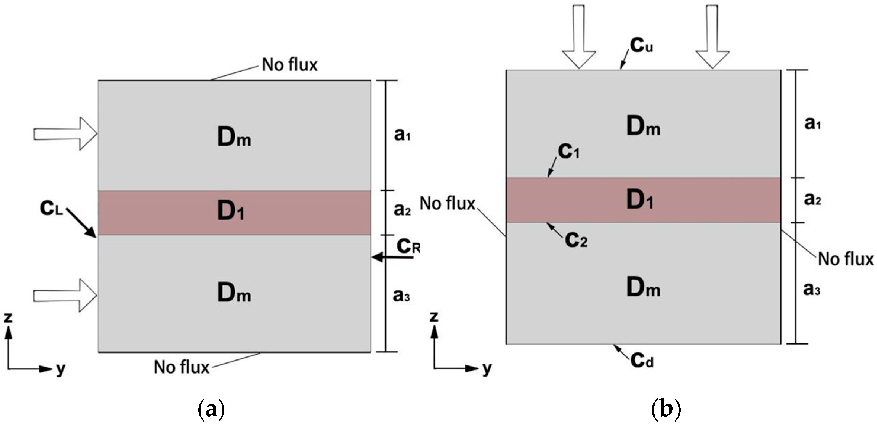
Figure 2.
3DPC simplified model (consider both the interlayer and inter-filament interfaces).

Figure 3.
Illustration of calculations for two models.

Figure 4.
Static analysis model.
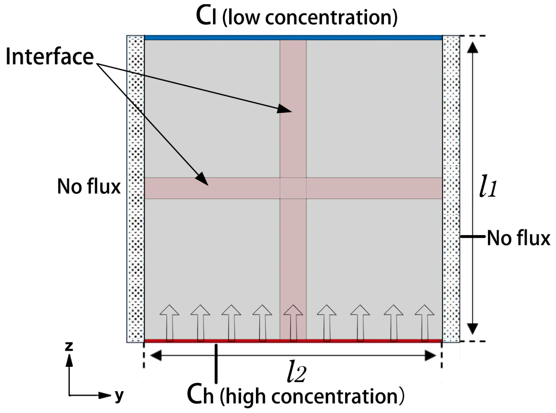
Figure 5.
Dynamic analysis model.
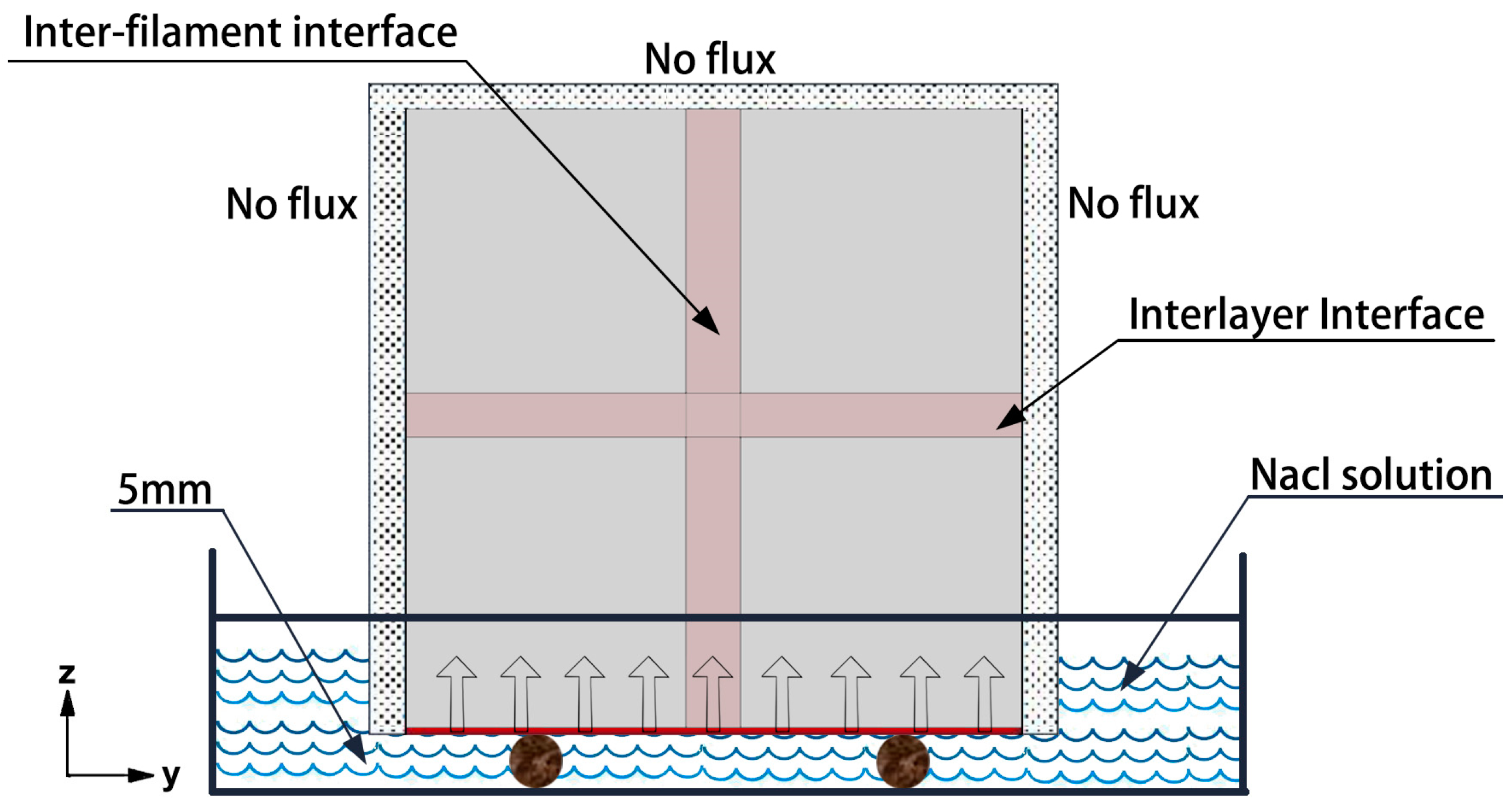
Figure 6.
Plot of interfacial diffusion coefficient with interfacial thickness.
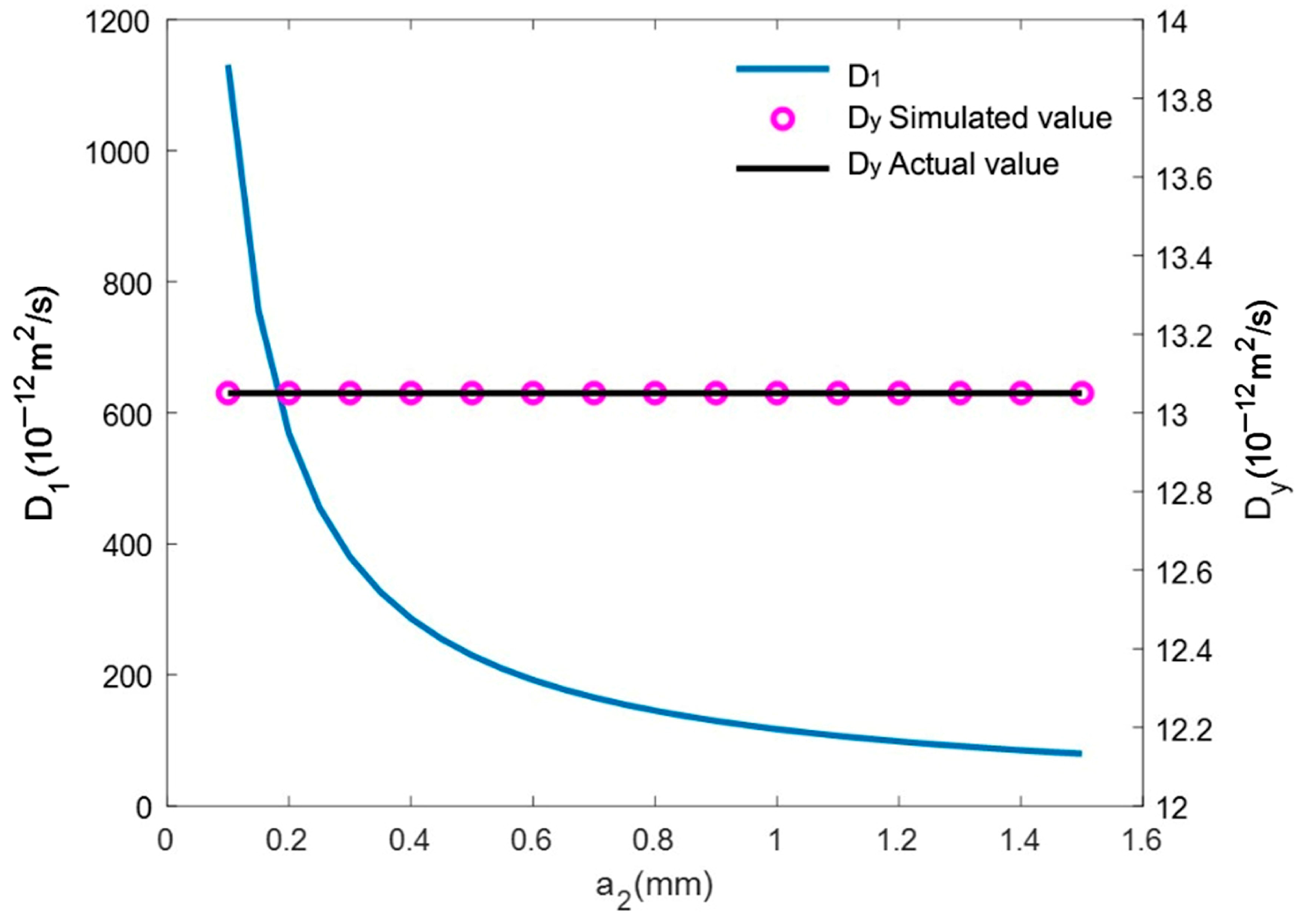
Figure 7.
Plot of interfacial diffusion coefficient versus interfacial thickness. (a) Variation of diffusion coefficient at the interlayer interface with the thickness of the interlayer interface. (b) Variation of diffusion coefficient at the inter-filament interface with the thickness of the inter-filament interface.

Figure 8.
Plot of the error of , , and in each scheme compared to the measured values. (a) Scenario 1; (b) Scenario 2; (c) Scenario 3; (d) Scenario 4.
Figure 8.
Plot of the error of , , and in each scheme compared to the measured values. (a) Scenario 1; (b) Scenario 2; (c) Scenario 3; (d) Scenario 4.
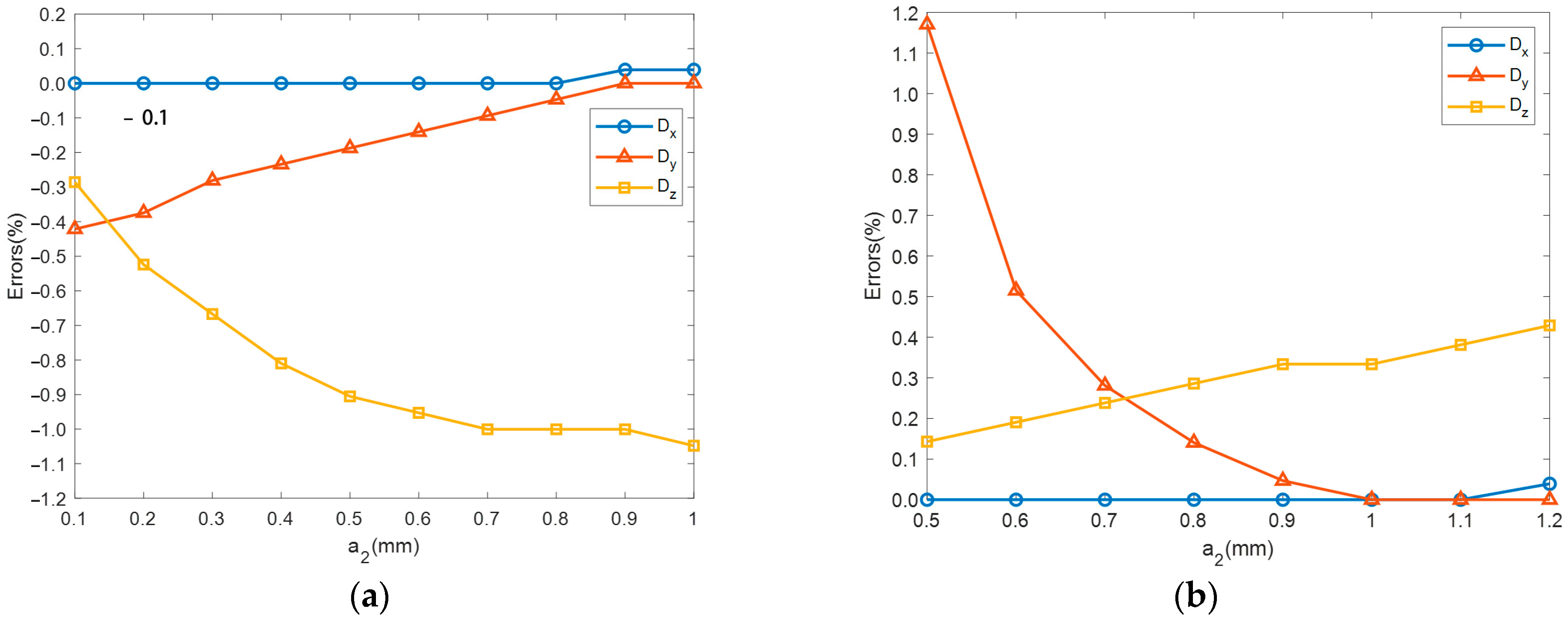
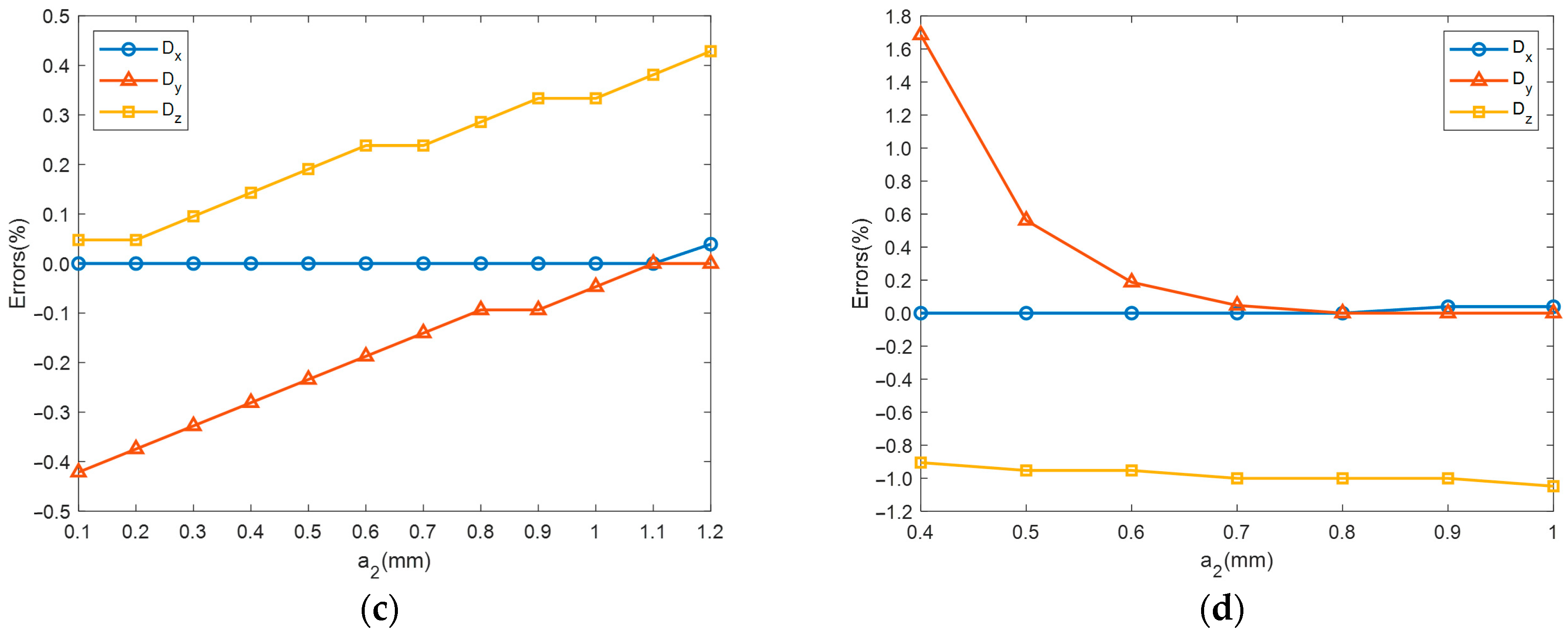
Figure 9.
Variation of the equivalent diffusion coefficient with material parameters. (a) ; (b) ; (c) .
Figure 9.
Variation of the equivalent diffusion coefficient with material parameters. (a) ; (b) ; (c) .

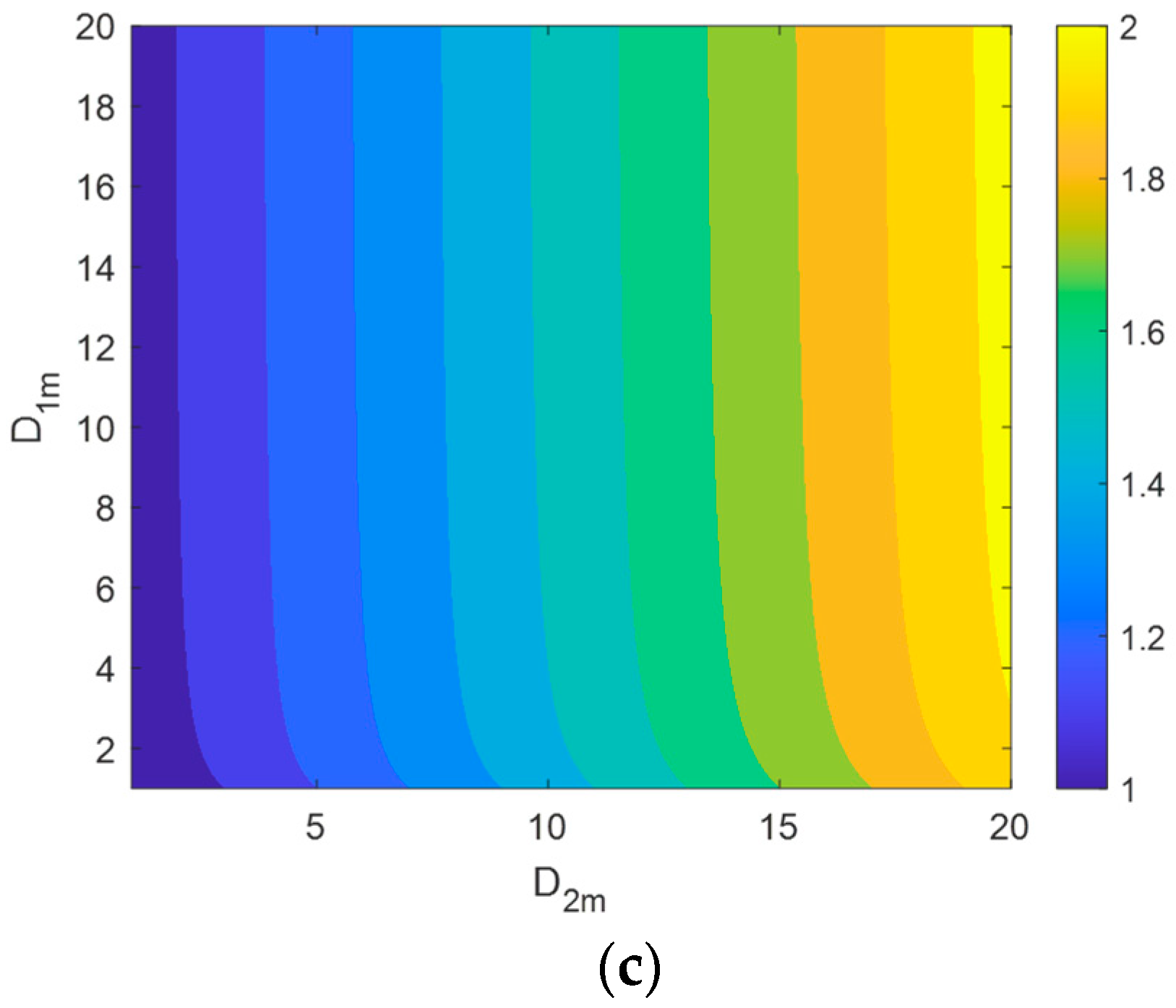
Figure 10.
Nondimensional equivalent diffusion coefficient variation with material parameters. (a) Curves of dimensionless equivalent diffusion coefficients as a function of D1m. (b) Curves of dimensionless equivalent diffusion coefficients as a function of D2m.
Figure 10.
Nondimensional equivalent diffusion coefficient variation with material parameters. (a) Curves of dimensionless equivalent diffusion coefficients as a function of D1m. (b) Curves of dimensionless equivalent diffusion coefficients as a function of D2m.
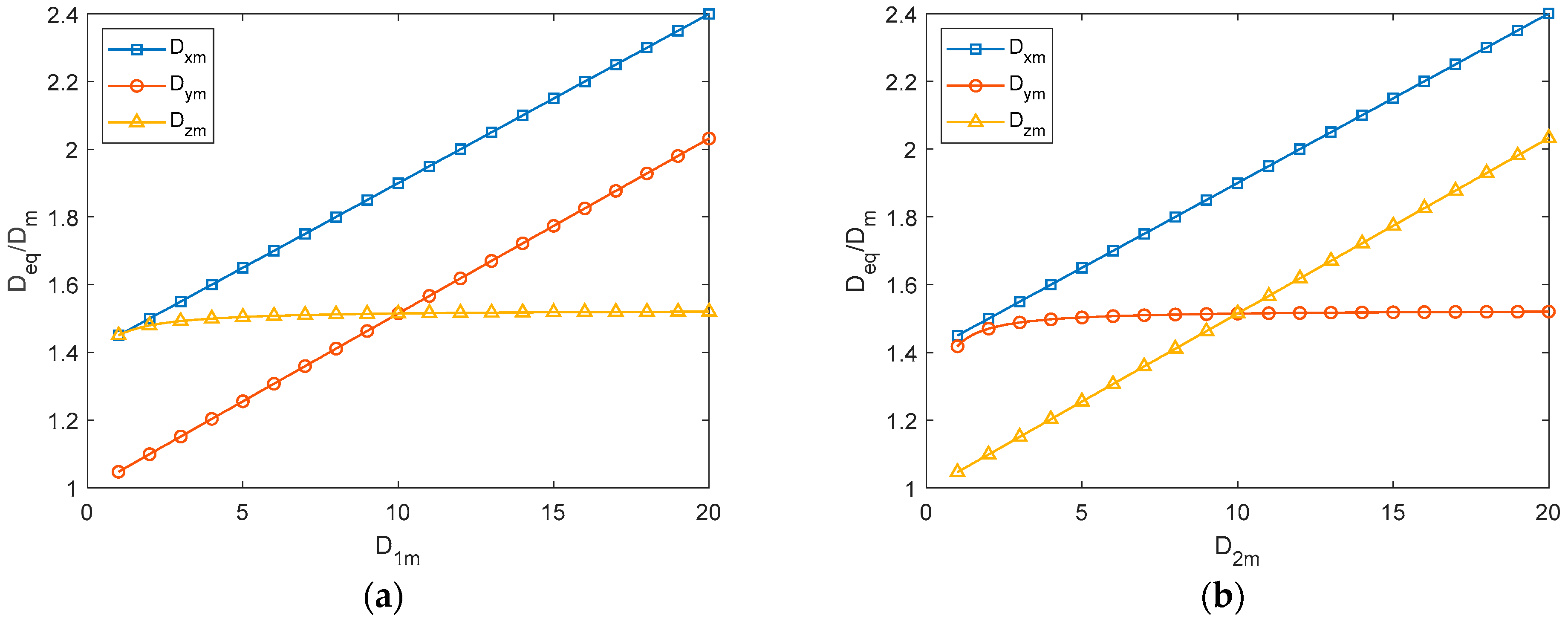
Figure 11.
Variation of the equivalent diffusion coefficient with structural parameters. (a) ; (b) ; (c)
Figure 11.
Variation of the equivalent diffusion coefficient with structural parameters. (a) ; (b) ; (c)
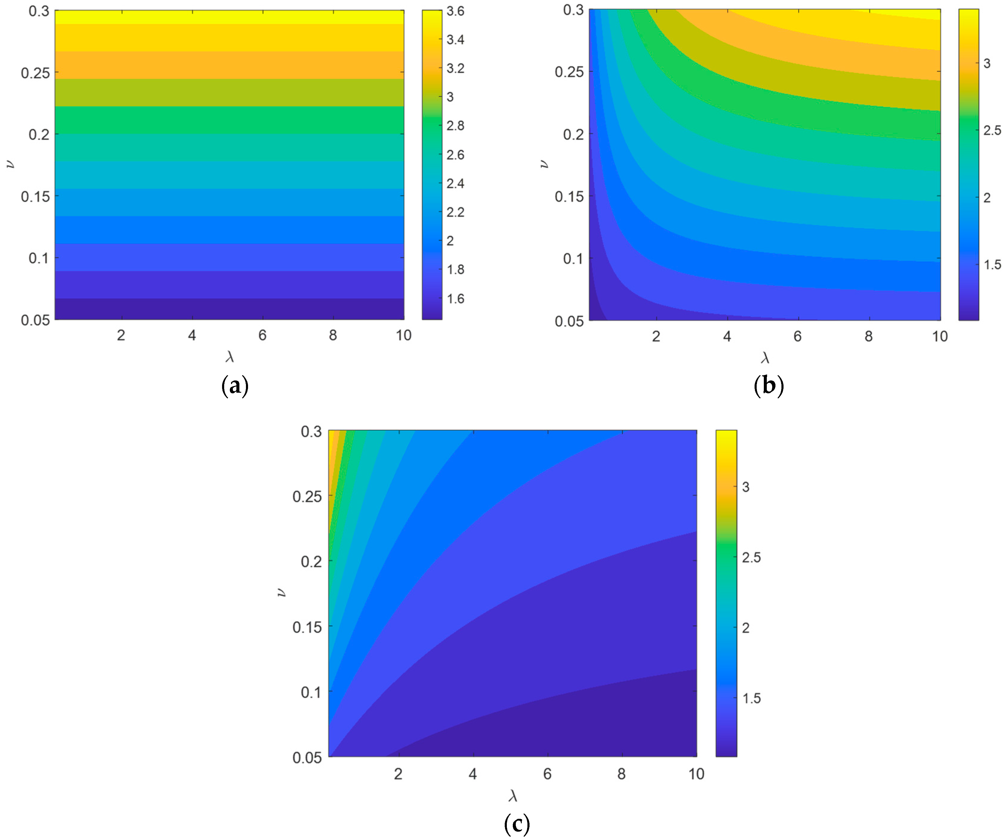
Figure 12.
Nondimensional equivalent diffusion coefficient variation with structural parameters. (a) Curves of dimensionless equivalent diffusion coefficients as a function of (b) Curves of dimensionless equivalent diffusion coefficients as a function of
Figure 12.
Nondimensional equivalent diffusion coefficient variation with structural parameters. (a) Curves of dimensionless equivalent diffusion coefficients as a function of (b) Curves of dimensionless equivalent diffusion coefficients as a function of

Figure 13.
Diffusion 30 d streamlines. (a) Model 1; (b) Model 2; and (c) Model 3.

Figure 14.
Chloride diffusion concentration maps for Models 1, 2, and 3 exit boundaries. (a) Chloride diffusion 5 d; (b) chloride diffusion 15 d; (c) chloride diffusion 40 d; and (d) chloride diffusion 200 d.
Figure 14.
Chloride diffusion concentration maps for Models 1, 2, and 3 exit boundaries. (a) Chloride diffusion 5 d; (b) chloride diffusion 15 d; (c) chloride diffusion 40 d; and (d) chloride diffusion 200 d.
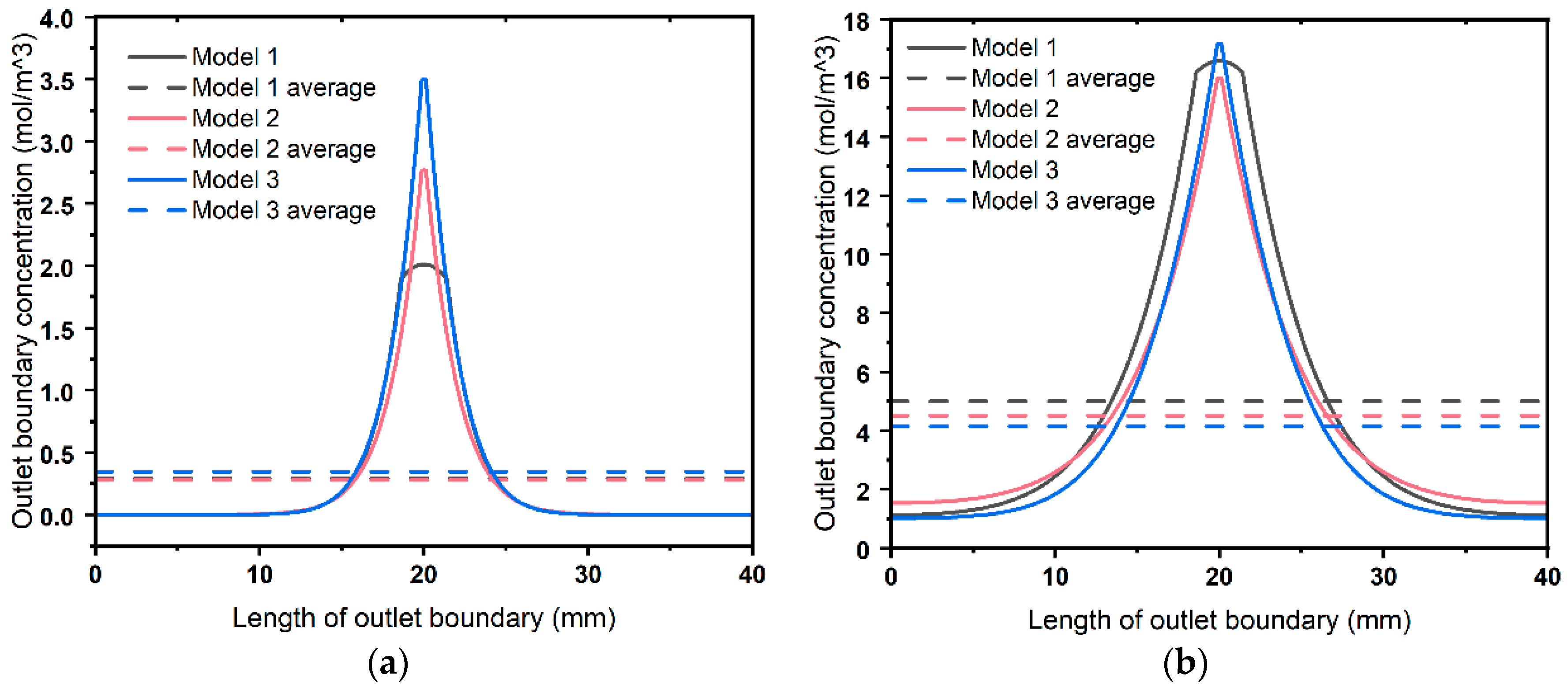
Figure 15.
Contour plots of critical concentrations for the three models. (a) Chloride diffusion 5 d; (b) chloride diffusion 15 d; (c) chloride diffusion 26.7 d; (d) chloride diffusion 27.4 d; and (e) chloride diffusion 40 d.
Figure 15.
Contour plots of critical concentrations for the three models. (a) Chloride diffusion 5 d; (b) chloride diffusion 15 d; (c) chloride diffusion 26.7 d; (d) chloride diffusion 27.4 d; and (e) chloride diffusion 40 d.

Table 1.
The main parameters of 3DPC in the literature test.
| Layers | Thickness of Single-Layer Matrix | Reference | ||
|---|---|---|---|---|
| 4 | 10 mm | 4.603 × 10⁻¹² m2/s | 13.05 × 10⁻¹² m2/s | J. Van Der Putten et al. [20] |
Table 2.
The main parameters of 3DPC in the literature test.
| Thickness of Single-Layer Matrix | Width of Single-Layer Matrix | Reference | ||||
|---|---|---|---|---|---|---|
| 6 mm | 20 mm | 15.03 × 10⁻¹² m2/s | 25.55 × 10⁻¹² m2/s | 21.36 × 10⁻¹² m2/s | 20.99 × 10⁻¹² m2/s | S. Surehali et al. [6] |
Table 3.
Four different systems of simultaneous equations schemes.
| Scenarios 1 | Scenarios 2 | Scenarios 3 | Scenarios 4 | ||
|---|---|---|---|---|---|
| Theoretical model | parallel connection | parallel connection | parallel connection | parallel connection | |
| Equation | (9) | (9) | (9) | (9) | |
| Theoretical model | parallel-then-series | series-then-parallel | parallel-then-series | series-then-parallel | |
| Equation | (13) | (17) | (13) | (17) | |
| Theoretical model | parallel-then-series | series-then-parallel | series-then-parallel | series-then-parallel | |
| Equation | (18) | (19) | (19) | (18) |
Table 4.
Parameter values of 3DPC computed under 4 scenarios.
| Scenarios 1 | Scenarios 2 | |||||
| (×10−12 m2/s) | (×10−12 m2/s) | (×10−12 m2/s) | (×10−12 m2/s) | |||
| 0.1 | 2.807 | 477.94 | 96.79 | No solution | ||
| 0.2 | 2.371 | 253.60 | 108.38 | No solution | ||
| 0.3 | 1.981 | 178.48 | 122.88 | No solution | ||
| 0.4 | 1.629 | 140.73 | 141.75 | No solution | ||
| 0.5 | 1.308 | 117.95 | 167.57 | 2.402 | 116.10 | 102.31 |
| 0.6 | 1.014 | 102.68 | 205.35 | 1.816 | 100.23 | 127.34 |
| 0.7 | 0.743 | 91.72 | 266.35 | 1.416 | 89.17 | 155.12 |
| 0.8 | 0.492 | 83.45 | 382.25 | 1.093 | 80.97 | 191.39 |
| 0.9 | 0.259 | 76.99 | 690.27 | 0.815 | 74.62 | 244.96 |
| 1.0 | 0.0418 | 71.80 | 4054.2 | 0.565 | 69.57 | 336.68 |
| 1.1 | No solution | 0.338 | 65.44 | 537.21 | ||
| 1.2 | No solution | 0.128 | 62.01 | 1353.8 | ||
| Scenarios 3 | Scenarios 4 | |||||
| (×10−12 m2/s) | (×10−12 m2/s) | (×10−12 m2/s) | (×10−12 m2/s) | |||
| 0.1 | 2.963 | 472.98 | 93.44 | No solution | ||
| 0.2 | 2.641 | 249.16 | 100.77 | No solution | ||
| 0.3 | 2.335 | 174.48 | 109.52 | No solution | ||
| 0.4 | 2.043 | 137.09 | 120.22 | 2.468 | 143.54 | 98.68 |
| 0.5 | 1.765 | 114.62 | 133.62 | 1.609 | 118.76 | 139.04 |
| 0.6 | 1.499 | 99.62 | 150.95 | 1.147 | 102.98 | 183.34 |
| 0.7 | 1.244 | 88.89 | 174.31 | 0.800 | 91.83 | 248.34 |
| 0.8 | 1.001 | 80.84 | 207.59 | 0.513 | 83.49 | 367.01 |
| 0.9 | 0.768 | 74.56 | 258.99 | 0.264 | 77.00 | 677.08 |
| 1.0 | 0.544 | 69.54 | 349.04 | 0.0419 | 71.80 | 4042.6 |
| 1.1 | 0.331 | 65.43 | 548.23 | No solution | ||
| 1.2 | 0.127 | 62.01 | 1363.8 | No solution | ||
Different Scenarios are bolded in the table.
Table 5.
The main modeling parameters of the three models.
| Number of Layers | Number of Strips | Matrix Thickness (mm) | Matrix Width (mm) | Interlayer Interface Thickness (mm) | Interlayer Interface Diffusion Coefficient (10−12 m2/s) | Interlayer Interface Horizontal Ion Transport Capacity (10−15 m3/s) | |
| Model 1 | 3 | 2 | 6 | 20 | 0.1 | 477.94 | 47.8 |
| Model 2 | 3 | 2 | 6 | 20 | 0.9 | 76.99 | 69.3 |
| Model 3 | 1 | 2 | 18 | 20 | \ | \ | \ |
| Inter-Filament Interface Thickness (mm) | Inter-Filament Interface Diffusion Coefficient (10−12 m2/s) | Inter-Filament Interface Vertical Ion Transport Capacity (10−15 m3/s) | |||||
| Model 1 | 2.807 | 96.79 | 271.7 | ||||
| Model 2 | 0.259 | 690.27 | 178.8 | ||||
| Model 3 | 0.259 | 690.27 | 178.8 | ||||
The names of the main parameters required in the table have been bolded.
Disclaimer/Publisher’s Note: The statements, opinions and data contained in all publications are solely those of the individual author(s) and contributor(s) and not of MDPI and/or the editor(s). MDPI and/or the editor(s) disclaim responsibility for any injury to people or property resulting from any ideas, methods, instructions or products referred to in the content. |
© 2024 by the authors. Licensee MDPI, Basel, Switzerland. This article is an open access article distributed under the terms and conditions of the Creative Commons Attribution (CC BY) license (https://creativecommons.org/licenses/by/4.0/).
Share and Cite
MDPI and ACS Style
Huang, T.; Peng, Z.; Wang, M.; Feng, S. Study on the Ionic Transport Properties of 3D Printed Concrete. Buildings 2024, 14, 1216. https://doi.org/10.3390/buildings14051216
AMA Style
Huang T, Peng Z, Wang M, Feng S. Study on the Ionic Transport Properties of 3D Printed Concrete. Buildings. 2024; 14(5):1216. https://doi.org/10.3390/buildings14051216
Chicago/Turabian StyleHuang, Tao, Zhongqi Peng, Mengge Wang, and Shuang Feng. 2024. "Study on the Ionic Transport Properties of 3D Printed Concrete" Buildings 14, no. 5: 1216. https://doi.org/10.3390/buildings14051216
Note that from the first issue of 2016, this journal uses article numbers instead of page numbers. See further details here.