1. Introduction
In recent years, there has been a global drive to reduce carbon emissions resulting from the production of energy through the burning of fossil fuels. One of the larger energy demands in the modern world results from the desire to control temperature through use of heating, ventilation and air conditioning (HVAC) systems, and light levels in working buildings [
1]. One of the best ways to reduce the need for HVAC systems is to improve the insulation of the building however most buildings are now constructed using large glazed areas. Glass is a cheap lightweight material that gives a desired aesthetic appeal however it is harder to control the heat flow through. Several types of glazing have been considered for the reduction of thermal loss or gain depending on the environment in which the system is to be used. In fact, the Passive house experiments carried out [
2] show that windows account for the greatest losses (~25 kWh(m
2a)
−1), as well as gains (~15 kWh(m
2a)
−1) in heat flow to and from a building.
The main environmental component, which must be considered when selecting a suitable glazing, is the average external environment, as this will dictate what role the material will play. In cold environments it is necessary to produce a material that will trap thermal energy with in the building. An example of this is low emissivity (Low-E) glazing, which reflects black body radiation thus reducing the loss of internal heat [
3]. Conversely, in high temperature environments there is a need for heat to be able to leave a building while also preventing heat from entering from the outside, this is achieved using absorbing glass that prevents the solar thermal energy from entering the building [
3]. However, many cities are in environments where the climate varies from hot to cold throughout the year for which a material with variable properties is desirable. This problem of temperature variation has led to research into “intelligent” glazing and in particular thermochromic materials. Thermochromic glazings display a change in the optical properties as a result in temperature change [
4,
5].
Some of the more promising thermochromic materials that are currently being investigated are based on VO
2. Monoclinic vanadium dioxide is an intrinsically thermochromic material with a transition temperature (T
c) of 68 °C for pure single crystal at which VO
2 undergoes a structural change from the monoclinic to the rutile phase. This change in phase has an effect on both the electrical and optical properties of the material. The monoclinic phase is a semiconductor that allows the transmission of IR radiation where as the rutile phase is metallic and is reflective to IR radiation. This value of T
c is clearly too high for use in building temperature; however, there have been several methods explored in attempts to alter this. It has been previously shown that the transition temperature can be significantly lowered through the introduction of metal ions into the VO
2 lattice [
6,
7,
8]. In fact, the most effective of the metals investigated has found to be tungsten as a 1 at% incorporation results in a 25 °C decrease in the T
c. Further to doping it has been found that the careful control of film growth and selection of synthetic route can be used to control the thermochromic properties through the introduction of varying amounts of film strain. Many methods have been investigated for the production of VO
2 thin films including, sol-gel [
9], physical vapor deposition [
10,
11] and chemical vapor deposition methods (CVD) [
12,
13,
14]. More recently work has been conducted on multilayer films [
15] and new deposition methods such as power impulse magnetron sputtering [
16] or oxidation of vanadium in unusual atmospheres [
17].
Previous modeling studies have shown that current VO
2 based materials do not live up to their theoretical potential but that an idealized thermochromic material can lead to great potential energy savings. In fact previous work has discussed the requirements for a perfect thermochromic window [
18,
19,
20]. Modeling has found that variable absorption in fact gives greater energy saving than variable reflectance also that carful control of emissivity also plays a vital role.
In this work the thermochromic transition is investigated with reference to the change in energy saving potential of several systems. Attention is paid to the variation of the transition temperature and, hysteresis width and gradient for the environments of Cairo, Paris and Moscow that represent hot, moderate and cold environments, respectively. The variation of the hysteresis and transition temperature are investigated, as they have all be shown to be different in VO2 films and so it is of importance to know which of these has the greatest impact on theoretical energy savings.
2. Results
The idealized spectra for the thermochromic systems all have an energy reduction due to the absorbing nature of the systems thus leading to an energy reduction even when no thermochromism is present. This intrinsic energy demand reduction can be quantified by modeling the systems using only the cold spectra. The results for these simulations (
Figure 1) can then be used to establish the energy demand reduction due to the variable heat mirror properties and those that arise from the absorbing properties.
2.1. Moscow
Figure 2 shows the change in environmental temperature for the daytime highs and nighttime lows in temperature throughout one year. It shows that although for a lot of the year the temperature is below a comfortable room temperature there is a period of summertime when it is above this temperature. This tells us that Moscow will have a summer cooling dominated environment and a winter heating dominated environment. It could, therefore, be inferred that during the winter a glazing in the cool transmissive state would be preferable (Temperature < T
c) and during summer a glazing in the hot reflective state would be preferable (Temperature > T
c).
Figure 3 shows the various energy load requirements for Moscow when using different glazing systems. In an environment where the main energy load will relate to cooling and heating it would be expected that the systems that could reflect the largest amount of solar energy when warm, stopping it from entering the building and transmit solar energy when cold allowing energy to enter the building would provide the greatest energy savings. It would be expected that the system that would best meet this criteria would be one with a low transition temperature and sharp gradient such that T
c < T.
The graphs in
Figure 3 show the percentage energy reductions for systems with different values of T
c, hysteresis width and hysteresis gradient. They are set with the clear–clear glazing system being used as a 0% energy saving baseline for use for comparison. The clear–clear glass energy load for the system was found to be 3877 kWh.
The graph in
Figure 3a shows the results from the simulations where T
c is set to 35 °C. In these simulations the worst performance comes from the system with the sharpest gradient and the widest hysteresis width (gradient 4, 15 °C width) giving a percentage saving of 7.8% (3574 kWh). The decrease in gradient causes an increase in energy saving of 4% (153 kWh) with the shallowest gradient and widest hysteresis width (gradient 1, 15 °C width) giving a saving of 11.8% (3421 kWh). Reducing the hysteresis width to the system with the narrowest width and sharpest gradient (gradient 4, 0 °C width) makes a change of 4.1% (158 kWh) to give a saving of 11.9% (3416 kWh). Reducing the steepness of the hysteresis leads to an increase in energy saving. The shallowest gradient (gradient 1, 0 °C width), gives 5.8% (224 kWh) increase in energy saving. The system with the shallowest gradient and narrowest hysteresis is the best performing giving a saving of 17.7% (3192 kWh).
Figure 3b shows the set of simulation results for the systems where T
c has been reduced to 30 °C. For this set of systems the worst performing is that with the steepest gradient and the widest hysteresis width (gradient 4, 0 °C width), which gives an energy saving of 9.8% (3497 kWh). Increasing the sharpness of the hysteresis gradient causes a decrease in energy consumption increasing the percentage energy saving to 12.5% (3391 kWh), an increase in saving of 2.7% (106 kWh). Reduction in hysteresis width also causes a reduction in the energy requirement with the system with the narrowest hysteresis and the shallowest gradient (gradient 1, 0 °C) giving a saving of 19.0% (3142 kWh). For the narrow hysteresis systems the hysteresis gradient has little effect with the greatest energy saving coming from the second shallowest gradient (gradient 2, 0 °C width), a saving of 19.5% (3119 kWh) a change of 0.5% (33 kWh).
Figure 3c shows systems with T
c set to 25 °C. Here the worst energy saving is afforded by the system with the widest hysteresis loop and sharpest gradient (gradient 4, 15 °C width) giving a saving of 12.8% (3381 kWh). Decreasing the slope of the hysteresis causes an improvement in energy saving with the shallowest gradient (gradient 1, 15 °C width) giving a saving of 13.3% (3362 kWh) although the best saving, for this hysteresis loop width, comes from the second shallowest gradient (gradient 2, 15 °C width). This gives a 13.7% (3348 kWh) saving, an increase in saving of 0.9% (33 kWh). Reduction in hysteresis width causes a reduction in energy load demand with the system with the narrowest and shallowest hysteresis (gradient 1, 0 °C width) giving a saving of 20.1% (3097 kWh), an increase in saving of 7.3% (284 kWh) compared to the worst performing system. For the systems with a narrow hysteresis, the increase in hysteresis gradient causes a decrease in the energy load demand with the best performing of all the systems being that with the narrowest and sharpest hysteresis (gradient 4, 0 °C width), which corresponds to an energy saving of 25.9% (2872 kWh), an increase of 5.8% (225 kWh) compared to the shallowest gradient.
Figure 3d shows the systems where T
c is at its lowest value, 20 °C For these systems the worst performance comes from the systems with a shallow gradient and a wide hysteresis loop (gradient 1, 15 °C width) giving a saving of 14.0% (3335 kWh). Changing to a system with a wide hysteresis but a sharp gradient (gradient 4, 15 °C width) causes an increase in energy saving of 2.2% (85 kWh) giving an energy saving of 16.2% (3250 kWh). A greater increase in energy saving is caused by reduction of hysteresis width with the system with a narrow hysteresis width and shallow gradient (gradient1, 0 °C width) giving a saving of 21.3% (3053 kWh), an increase of 7.3% (282 kWh) compared to the worst performing system. The system with the sharpest gradient and the narrowest hysteresis width (gradient 4, 0 °C width) is the best performing of the systems with the gradient variation increasing the saving by 8.5% (332 kWh) with the total energy saving being 29.8% (2721 kWh).
The results in
Figure 3 show that the worst systems for this environment are ones with a high values T
c and with a sharp wide hysteresis (T
c = 35 °C, gradient 4, 15 °C width). The best performing system is that with a sharp, narrow hysteresis width with a low value for T
c (T
c = 20 °C, gradient 4, 0 °C with). At low values of T
c the sharp wide hysteresis width allows a stretching of the thermochromic effects as the width allows a greater range of T
c values and still a quick switch between effects that would be favored in a variable temperature environment.
2.2. Paris
Figure 4 shows the temperature profiles for the monthly highs and lows throughout one year in Paris. It shows that, from April until October, the highest temperature is greater than a comfortable room temperature (21–23 °C) this means that there is a daytime requirement for cooling. During the rest of the year there will be heating requirements.
Figure 4 indicates that this is a variable temperature environment and will have both cooling and heating requirements. The cooling dominated environment (summer) means that the thermochromics will be most efficient in the hot state (temperature > T
c). In the heating dominated environment (winter) the thermochromics will work best in the cold mode (T
c < temperature). For the rest of the time, the thermochromics will need to switch between the two states depending on the time of day.
The graphs in
Figure 5 show the percentage reduction in energy demand for systems with varying values of T
c, hysteresis width and hysteresis gradient. The actual values for the energies are shown in brackets after each quoted percentage. Clear–clear glass systems are set as a 0% saving baseline. The system with a clear–clear glass window required an energy load of 2695 kWh of power.
The results in
Figure 5a show the % energy saving for systems with a value of T
c of 35 °C. In these systems the worst performing are those with sharp hysteresis gradient (gradient 4) and a wide hysteresis loop (15 °C) giving a 13.3% (2335 kWh) energy saving. When the hysteresis gradient is reduced to its shallowest (gradient 1) the energy saving increases to 18.3% (2201 kWh), a change of 5% (134 kWh) in energy demands. Decreasing the hysteresis width also reduces the energy demand with the system with the sharpest gradient (gradient 4) and narrowest hysteresis width (0 °C) resulting in a saving of 18.8% (2188 kWh), a saving of 5.5% (147 kWh) compared to the worst system. The system that performs the best is the one with a shallow hysteresis gradient (gradient 1) and a narrow hysteresis width (0 °C), resulting in a saving of 26.8% (1972 kWh). Increase in hysteresis width to the widest system (15 ° width, gradient 1) causes an increase in energy demand of 8.5% (229 kWh). Unlike the systems with a wide hysteresis the systems with narrow hysteresis have the opposite relationship with respect to gradient variation. As the gradient becomes steeper, the energy saving decrease with the sharpest gradient (gradient 4) giving a saving of 18.8% (2188 kWh) a decrease in saving of 8% (216 kWh). In these systems both hysteresis width and gradient have a similar effect on the energy saving potential of the glazing systems.
Figure 5b shows the graph representing the energy saving % of the systems with T
c set to 30 °C. For this set of systems the best performing is that with a narrow hysteresis width (0 °C) and a medium sharp gradient (gradient 2) giving a 29.1% (1911 kWh) energy saving. The shallower gradient has little effect on the energy saving for systems with a narrow hysteresis width; the shallowest gradient system (0 °C width, gradient 1) gives a saving of 29% (1914 kWh), a decrease of 0.1% (3 kWh). For the systems with wider hysteresis (15 °C) the change in gradient again has little effect on the energy saving properties of the glazing systems with the sharpest gradient (gradient 4) giving a saving of 16% (2263 kWh) and the shallowest gradient (gradient 1) giving a saving of 19.4 (2172 kWh), a difference of 3.4% (91 kWh). The greatest effects on energy saving potential for these systems comes from variation of the hysteresis width, the sharpest thinnest hysteresis (gradient 4, 0 °C width) giving a saving of 29% (1914 kWh) and the sharpest widest hysteresis (gradient 4, 15 °C width) giving a saving of 16% (2263 kWh), a difference of 13% (349 kWh).
The graph shown in
Figure 5c is the results for systems with T
c set to 25 °C. The worst energy saving is afforded by the system where gradient is at its maximum and the hysteresis widest (gradient 4, 15 °C width) where the energy saving is 19.8% (2161 kWh). By reducing the gradient the percentage saving is slightly increased until the second shallowest gradient (gradient 2, 15 °C width), which affords a saving of 20.7% (2137 kWh) an increase in saving of 0.9%. Increasing the gradient further causes a slight decrease in efficiency. When the hysteresis width is reduced to its minimum the energy efficiency is increased with the best performance coming from the steepest gradient and narrowest hysteresis width (gradient 4, 0 °C width) giving a saving of 37.3% (1691 kWh), an improvement of 17.5% (470 kWh) from the worst system. With the narrowest hysteresis width simulations the gradient variation has a greater affect on the percentage savings although it is still not a great affect with the shallowest gradient (gradient 1, 0 °C width) giving a saving of 31% (1858 kWh), a variation of 6.3% (167 kWh).
Figure 5d shows the system with T
c set to 20 °C for this set of simulations the worst performing system is where the hysteresis loop has the shallowest gradient and widest hysteresis width (gradient 1, 15 °C width). This system affords an energy saving of 21.6% (2114 kWh). Increasing the steepness of the hysteresis the energy saving is increased with the steepest gradient (gradient 4, 15 °C width) affording a saving of 24% (2048 kWh), an increase of 3.4% (66 kWh). Reduction of the hysteresis width has a greater affect on the energy saving potential with the system with shallow gradient and narrow hysteresis width (gradient 1, 0 °C width) giving a saving of 33.2% (1800 kWh) an improvement of 11.6% (314 kWh) compared to the worst system. The most efficient film for the system is that with the sharpest gradient and narrowest hysteresis loop (gradient 4, 0 °C width), giving a saving of 42.8% (1540 kWh) an improvement of 9.6% (260 kWh) from the change in gradient from the shallowest.
Comparing the graphs in
Figure 10 the systems with a low T
c, the best performance comes from the systems with a narrow hysteresis width and a sharp gradient. As the value of T
c is increased the increased performance comes from the systems where the hysteresis width is minimized, but the gradient at its shallowest this is due to the higher T
c values being spread over a larger range making the transition occur at lower temperatures thus increasing the potential of reflective properties.
2.3. Cairo
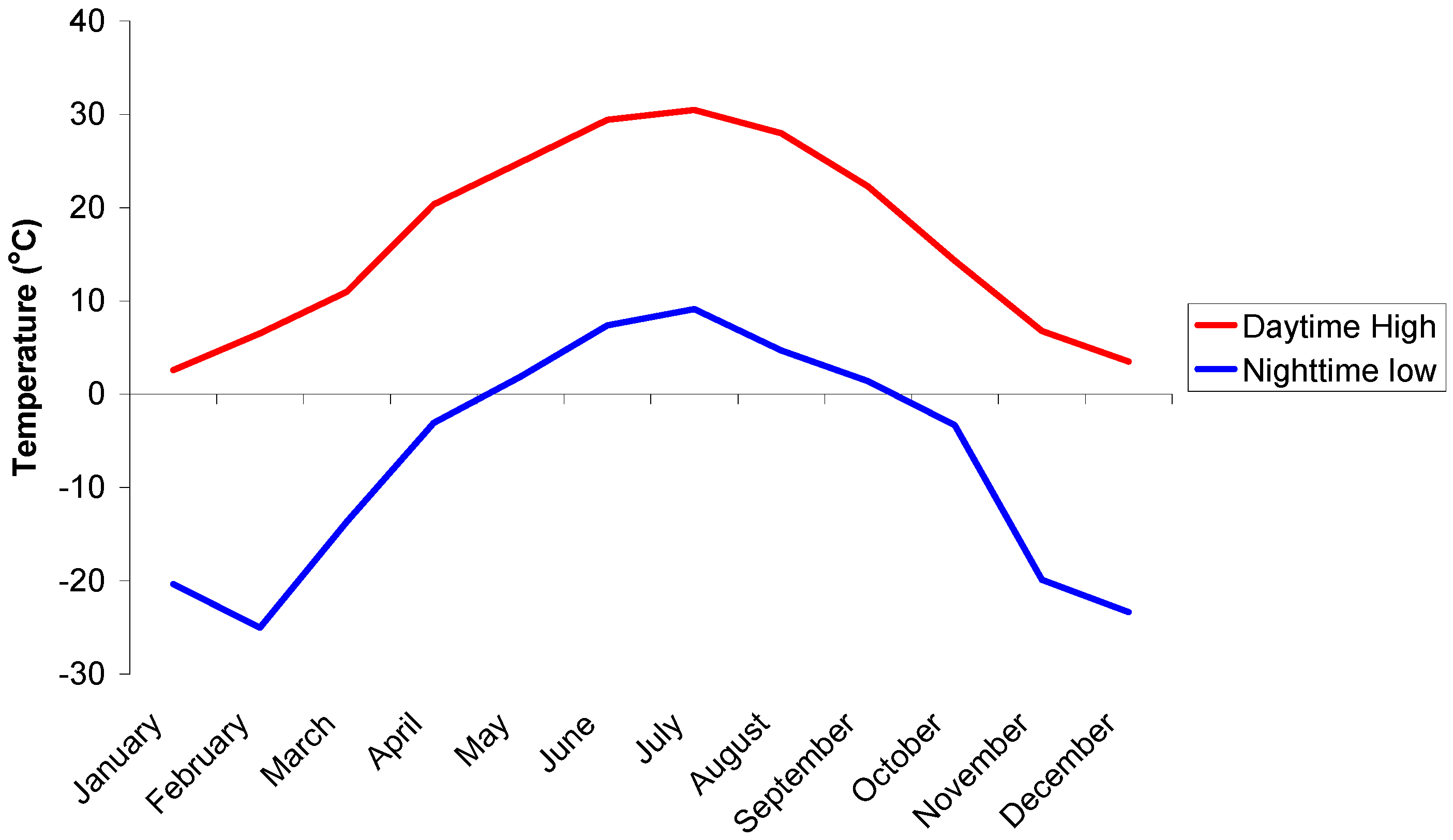
Figure 6 shows the temperature profiles for the monthly highs and lows throughout one year in Cairo. It shows that for almost the entire year, the highest temperature is greater than a comfortable room temperature (21–23 °C). This means that there is a constant daytime requirement for cooling.
Figure 6 shows different glazing systems modeled for the environment in Cairo, Egypt. The average temperature, taken from the weather file, across the year is 22 °C meaning that this is a cooling dominated environment. The cooling dominated environment means that the thermochromics will be most efficient in the hot state (temperature > T
c) it can therefore be assumed that the thermochromic with the lowest transition temperature will perform the best as they will spend the greatest amount of time in the hot state and reflect the most solar energy
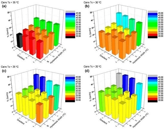
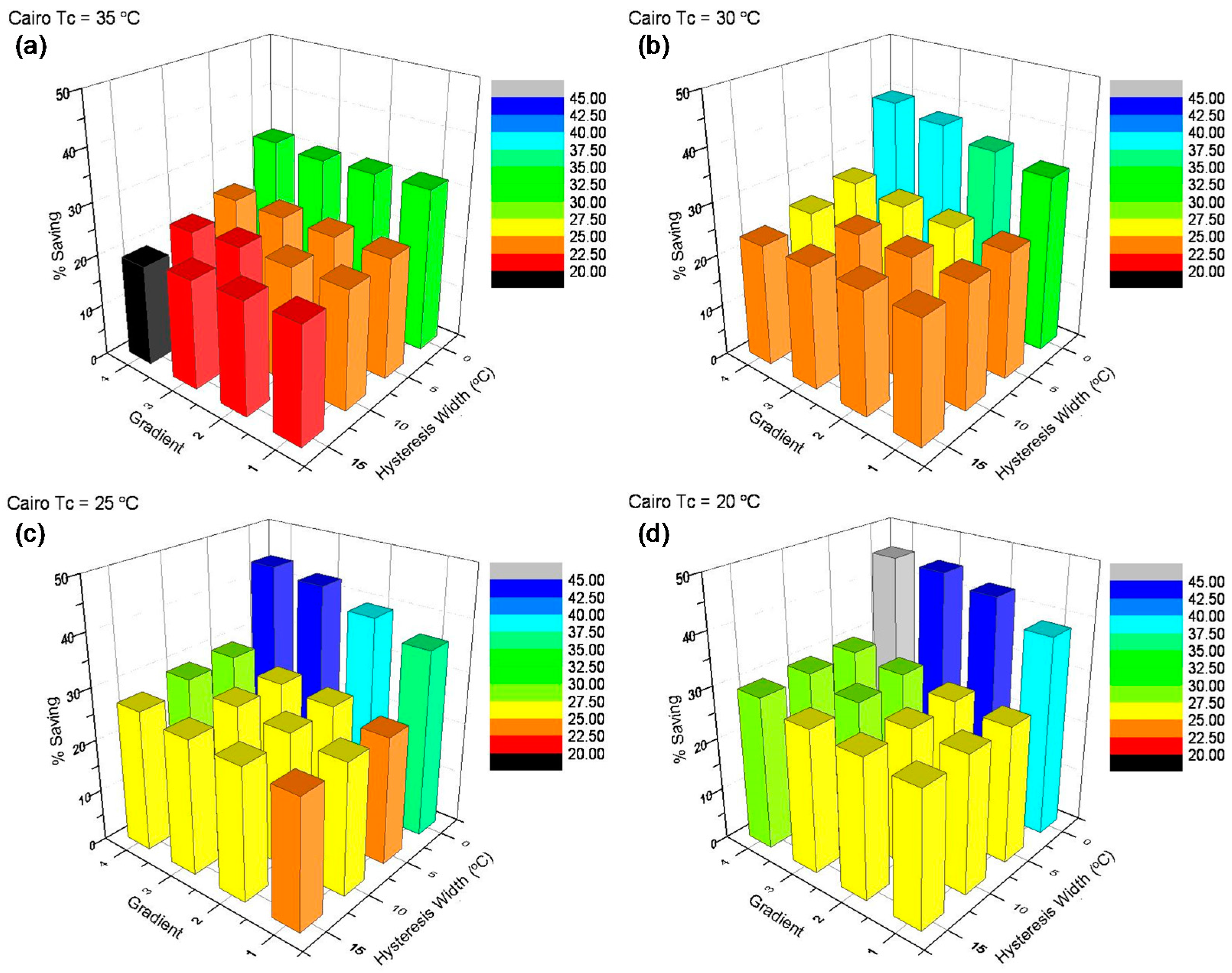
The graphs in
Figure 7 show the percentage reduction in energy demand for systems with varying values of T
c, hysteresis width and hysteresis gradient. The actual values for the energies are shown in brackets after each quoted percentage. Clear–clear glass systems are set as a zero-percent-saving baseline. The system with a clear–clear glass window required an energy load of 3966 kWh.
Figure 7a shows the modeled system results for Cairo where the thermochromic systems have the highest value for T
c (T
c = 35 °C). For the set of systems shown in
Figure 11, the highest percentage energy saving compared to clear–clear glass results from the system where the hysteresis width is minimized and the gradient at its steepest. The reduction of energy due to the reduction in hysteresis width has the greatest effect for systems with the sharpest gradient (gradient 4). For these examples, the change is 12% (491 kWh) with the greatest saving being 31.8% (2706 kWh) and the lowest being 19.4% (3197 kWh). The smallest effect of hysteresis width variation occurs for systems with the shallowest gradient (gradient 1). The widest hysteresis width (15 °C) gives an energy reduction of 22.2% (3084 kWh) and the thinnest hysteresis width (0 °C width) gives a saving 31.6% (2712 kWh), leading to a 9.4% (372 kWh) variation across the systems. The greatest variation in gradient effect on these systems occurs when hysteresis width is maximized (15 °C width) in this case the sharpest gradient (gradient 4) gives a saving of 19.4% (3197 kWh) and the shallowest gradient (gradient 1) gives a saving of 22.2% (3084) a variation of 2.8% (113 kWh) across the gradients. The narrowest hysteresis width (0 °C width) with the sharpest gradient (gradient 4) gives a saving of 31.8% (2706 kWh) and the shallowest gradient (gradient 1) gives a saving of 31.6% (2712 kWh), a difference of 0.2% (6 kWh). In this situation, the lowest percentage saving comes from gradient 3, 31.0% (2738 kWh) and the highest from gradient 1. These give a variation of 0.8% (32 kWh) between them. This shows that for this transition temperature the hysteresis width variation has a greater effect on the energy saving properties than the hysteresis gradient variation.
The graph in
Figure 7b shows the situation where the T
c value has been decreased to 30 °C in this situation the systems with a wide hysteresis width (15 °C width) are little effected by variation in gradient with a difference of 0.2% (6 kWh) between the second steepest gradient (gradient 3) and the shallowest gradient (gradient 1). This represents savings of 23.5% (3035 kWh) and 23.3% (3041 kWh) respectively. The gradient variation has a more noticeable effect on the energy saving as hysteresis width is decreased. It is most noticeable when the hysteresis width is minimized (0 °C width), steepest gradient (gradient 4) gives a saving of 39.7% (2391 kWh), the shallowest gradient (gradient 1) a saving of 33.8% (2626 kWh). This is a variation of 5.9% (235 kWh). The greatest energy saving at this value of T
c is for the sharpest gradient and the narrowest hysteresis width (gradient 4, hysteresis width 0 °C), a saving of 39.7% (2391 kWh). For the system with very sharp gradient (gradient 4) the effect of hysteresis width variation is a change of 16.4% (649 kWh) in energy saving when going from the widest hysteresis width (15 °C width, 23.4%, 3040 kWh) to the narrowest hysteresis (0 °C, 39.7%, 2391 kWh). For the shallowest gradient (gradient 1) the variation of hysteresis width gives a change in energy saving of 10.5% (415 kWh) when going between the widest hysteresis (15 °C, 23.3% saving, 3041 kWh), and the narrowest hysteresis width (0 °C, 33.8% saving, 2626 kWh). This implies that for systems with a T
c of 30 °C the hysteresis width has the greatest effect on the overall glazing performance.
The graph in
Figure 7c shows the results for a glazing with T
c = 25 °C in this set of simulations the worst performing system is that with the widest hysteresis width (15 °C width) and shallowest gradient (gradient 1), a saving of 24.4% (2996 kWh). When the hysteresis gradient becomes steeper the percentage energy saving is increased. The best performing system with a hysteresis width of 15 °C is that with the steepest gradient (gradient 4), giving a 27.0% (2895 kWh) saving in energy, an improvement of 2.6% (101 kWh). The systems with the sharpest gradient (gradient 4) have a difference in saving of 16.8% (667 kWh) between the widest hysteresis (15 °C width) saving 27% (2895 kWh) and narrowest hysteresis (0 °C width) saving 43.8% (2228 kWh). The best performing system is that with the narrowest hysteresis width and sharpest gradient, giving a saving of 43.8% (2228 kWh). As the gradient is reduced, for the systems without a hysteresis width (0 °C width), the energy efficiency is decreased. The difference in energy saving between shallowest (gradient 1) and sharpest gradient (gradient 4) is 7.8% (309 kWh).
Figure 7d shows the energy savings for the simulations where T
c = 20 °C. These simulations show the best performing systems are those where the gradient is sharpest (gradient 4) and the hysteresis is thinnest (0 °C width) giving a saving of 45.3% (2170 kWh). The worst performing in these systems is that where the gradient is shallowest (gradient 1) and the width maximized (15 °C width) giving a saving 25.5% (2953 kWh). This shows that the difference in energy saving between best and worst performing systems is 19.8% (783 kWh). The biggest effect caused by gradient variation alone occurs when the hysteresis width is minimized (0 °C width). The steepest gradient (gradient 4) gives a 45.3% (2170 kWh) saving, and the shallowest (gradient 1) a saving of 38.2% (2451 kWh), a difference of 7.1% (281 kWh). The biggest effect caused just by hysteresis width variation is for the systems with gradient 3. In this case the maximum percentage saving occurs where the hysteresis width is minimized (0 °C width), a saving of 44.7% (2193 kWh). The least saving occurs when hysteresis width is maximized (15 °C width), a saving of 27.3% (2884 kWh). This gives a difference of 17.4% (691 kWh). This implies that for this case the hysteresis width has a greater effect on overall performance than the hysteresis gradient although only marginally.
When comparing low T
c values in
Figure 7, the most energy efficient systems are those with a sharp gradient (gradient 4) and a narrow hysteresis width (0 °C width). For situations where T
c is high, the best systems are still those with a narrow hysteresis width and a shallow gradient. This can be attributed to the fact that for systems with a high T
c the switch to the reflective state requires a higher environmental temperature. The larger range afforded by the reduced gradient allows the systems to enter the reflective stage at a lower temperature by spreading the switch over a larger temperature range. The overall best performing system was that with a low T
c (T
c = 20 °C), a narrow hysteresis loop (0 °C width) and a sharp gradient (gradient 4). This system gave a maximum saving of 45.3% (2170 kWh) when compared to the same system using a clear–clear glass window.
3. Discussion
The theoretical thermochromic systems all evidence a reduced energy requirement when compared to the clear–clear glass system for heating, lighting and cooling loads (
Table 1), as well as out performing both of the industrial standards. Throughout the data for all environments, it can be observed that there are some general trends. In all of the modeled environments it can be seen that the greatest energy saving can be attributed to the thermochromic systems with the lowest transition temperature and the sharpest gradient with the narrowest hysteresis width. In systems with these “best” properties, it is seen that of the three variables transition temperature reduction has the greatest impact on the overall energy saving potential. Reduction in the thermochromic transition temperature, from 35 to 20 °C leads to increases in the potential energy saving of between 15%–30% corresponding to a 1.5%–3% saving for each 1 °C reduction in the transition temperature.
As was mentioned the best performances were found to result from the systems wit the sharpest gradients. The increase in the hysteresis gradient (gradient 1 to gradient 4) has a potential of giving potential saving increases of between 7%–15% which corresponds to a 0.3%–0.6% energy saving for each 1Δ%T/ΔT (°C) change in transition gradient. If is further seen that the greatest effect of gradient variation on energy saving is more substantial when going from gradient 1 to 4, in fact, typically an extra 5%–10% improvement in energy demand is observed when reducing the hysteresis gradient from −1 to −5Δ%T/ΔT (°C). These values correspond to a saving of 1%–3% for each 1Δ%T/ΔT (°C) making this region the more influential area of gradient variation. This effect is correlated to the rate at which the hot and cold states can cycle allowing for maximum efficiency in allowing for the use of the most appropriate glazing properties. It should be noted that for gradients steeper than −5Δ%T/ΔT (°C) this effect rapidly plateaus.
In all systems the greatest energy demand reductions are afforded from the systems with the narrowest hysteresis loop. This effect is attributed to the wider hysteresis causes a “stretching” of the transition temperature leading it to be effectively higher while heating and lower when cooling. This effect reduces the systems speed at which the thermochromic transition can be achieved. This effect of hysteresis width can be considered in two parts, as the data shows that there is a jump in efficiencies when increasing the width from 0 to 5 °C. In fact, this variation causes a drop in efficiency of between 7%–20% that corresponds to 1.4%–4% change in efficiency for every 1 °C variation in the hysteresis width. The further variation in the hysteresis width from 5–15 °C has less of an effect on the energy saving potential giving a change of 2%–5% or a change of 0.2%–0.5% change in efficiency for each change of 1 °C in the hysteresis width. The dramatic increase in efficiency afforded to the systems when reducing the hysteresis width from 5–0 °C is attributed to an increased switching ability from hot to cold states of the systems allowing a faster “reaction” to the variation in outside temperature.
As discussed, Moscow is considered to be a cold climate and therefore and would therefore main benefit from a material is the transmission of heat energy during the winter period when cold and secondly the reflection of heat during the hot summer period. In fact, it was found that the system that afforded the greatest energy savings was that with a sharp hysteresis gradient (gradient 4) narrow hysteresis width and low transition temperature which give a saving of 30% compared to the clear–clear system giving a total energy demand of 2721 kWh. This energy saving improvement is also grater than that afforded by the two industrial standards that have energy loads of 3352 and 3391 kWh for absorbing glass and silver sputtered heat mirror glass, respectively. For this low temperature environment it is found that at higher transition temperatures the most efficient systems still have a narrow hysteresis however now a shallower gradient is preferable. The system with a high transition temperature narrow and sharp hysteresis the energy saving is 11.9% where as the greatest saving is afforded by the system with a narrow shallow gradient resulting in a17.7% saving. This shallow gradient allows a “spreading” of the thermochromic transition so while the transition temperature is high the thermochromic effect can be accessed at lower temperatures where as with the steeper gradients the transition is much more focused at the transition temperature point.
Paris has a more variable climate with cold winters and hot summers with a period (spring/autumn) of variable temperatures between them. An environment such as this would benefit from a system, where the state of the material can switch between hot and cold states effectively regulating the solar energy entering the building as a close representation to the external environment. The modeling results show that the best system for this environment is that with a low transition temperature and a sharp narrow hysteresis that has an energy load of 1691 kWh, which can give a potential saving of 43% compared to the blank glass system. This is also an improvement on both of the industrial standards also modeled where the absorbing glass and silver sputtered glass had energy loads of 2031 and 2162 kWh, respectively, that correspond to 25% and 20% energy improvements on clear–clear glass. The sharp narrow hysteresis with a low transition temperature is what is expected as it allows for rapid switching between transmitting and reflecting states near the room temperature and allowing for the best control correspondence to the external temperature and fully utilizing the available solar radiation. As with the cold environments it was seen that when the transition temperature was reduced the hysteresis shape favored was altered. As discussed at a low transition temperature a sharp narrow hysteresis is favorable however at high transition temperatures the preferred system is that with a narrow shallow hysteresis. In fact, for the Paris environment, when Tc is set to 35 °C, a sharp narrow hysteresis gives an energy saving of 18.8% where as a shallow narrow hysteresis gives a saving of 26.8% compared to the clear–clear system.
Cairo is a hot environment where the dominating requirement is to reduce the solar heat gain thus reducing the cooling energy loads. This would be best achieved through the prevention of infrared solar radiation from entering the building, an effect that can be best achieved through either reflection or absorption of the radiation. As with the other environments the best performing systems are those with a narrow sharp hysteresis with a low transition temperature. This best performing system had an energy demand of 2170 kWh, a saving 45.3% compared to the clear–clear glass system. This system is also better than both the absorbing glass and silver sputtered heat mirror glass, which had energy loads of 715 kWh and 1106 kWh, respectively, that correspond to savings of 18.7% and 27.9% compared to the clear–clear system. The good performance for the systems with low Tc and a sharp narrow hysteresis is as expected for hot environments as it allows the system to rapidly enter the reflecting state rapidly and therefore effectively blocks the infra red radiation from entering the building. Unlike the previous environments it was found that at higher transition temperatures a change in the hysteresis gradient has little effect on the energy saving potential. This is due to the following trade off: the shallower gradient allows more reflection at lower temperature but makes the more reflective state hard to reach, whereas the sharp gradient allows a quick switch to the reflective state when Tc is reached therefore immediately reaching the maximum reflection of infra red solar radiation.
Overall, the results show that the greatest possible energy savings are achieved for the hot environment (Cairo), although significant savings were also achievable for the other two environments as well. The results indicate that the systems are effective as intelligent glazing and can outperform industry standards. It has been seen that for all environments the best system is that with a sharp narrow hysteresis with a transition of 25 °C.
4. Materials and Methods
Energy modeling and analysis was performed on the simulation software EnergyPlusTM developed at Lawrence Berkley National Laboratory and US Department of Energy. EnergyPlusTM software is an energy analysis and thermal load program allowing the user to input a building based on its dimensions, physical construction, usage and mechanical systems present. The soft ware has two modes of input/editing either through the soft ware interface or by use of a text file. This work used Energy PlusTM version 5.0.
4.1. Building Parameters
The building set up was of a simple single room assumed to be within a building such that only on wall was exposed to the external environment. The dimensions of the model were 6 m × 5 m × 3 m (length × width × height) and was orientated such that each wall was perpendicular to either north south or east west with the external wall being the south facing. The external wall of the building was modeled such that the wall was covered by a window for 99% a schematic of the model can be seen in
Figure 8. A 99% glazed façade was chosen as to be representative of modern office blocks. The model is a mid-floor office in a multi-floor complex and is therefore buffered above and below by conditioned spaces for this reason the ground temperature would have no effect on the models performance. The choice of the ground temperature was taken to be 18 °C throughout the year not to reflect the ground temperature but to be representative of a further buffering zone below the model. All walls other than external were assumed to be adiabatic with a constant temperature of 18 °C.
The materials shown in
Table 2 are the standards used in EnergyPlus and the data is taken straight from the program defaults.
Table 3 shows how each of the building components were constructed and the properties of the materials are shown in
Table 3. The window of the building was the only part of the structure that was modified through out the simulations, and this was done by changing the glazed layer in the system. The air gap in the windows was 12 mm and the glazing was modeled so as to be on the inside face of the outer pane of glass in all cases.
4.2. Building Conditions
The internal conditions of the building were chosen so as to represent the conditions found in an office bloc. The internal temperature, controlled by the inbuilt HVAC model, was chosen to be between 19–26 °C to allow for comfortable working conditions. The required luminance in the building was taken to be 500 lux, this corresponds to a lighting load of 400 W. The lights are allowed to be fully dimmable and will be reduced when adequate light can enter through the window. The lighting was fully dimmable between 0%–100% and was automated and zoned. The casual heat gain (equipment and people) is set to 500 W in total. The ventilation rate was 0.025 m3·s−1 to simulate an office like building the occupancy was set to be from 8:00–18:00, Monday–Friday.
4.3. External Conditions
External conditions were controlled by use of weather files. The weather files give a yearly reading of the conditions in various locations around the world with all required information, i.e., solar gains, outside temperature, etc.
4.4. Model Limitations
The main limitation to this model is its simplicity and its directional confinements, assuming a south facing façade. The model could be expanded upon by introduction of further units with different orientations or window sizes. The model is also limited, as the building will not be fully optimized for all climates. In the different climates, warmer, cooler, and variable, the materials and insulating would vary for optimization. The materials would also vary due to local materials available, construction techniques and area specific aesthetics. The use of kWh for the output of energy is not necessarily the most accurate measure of energy usage as different methods may be used to produce different energy inputs, which will have different energy demands associated to them. These limitations have been minimized by using results obtained from plain glass as either comparisons or as a base line for percentage improvements therefore allowing for the change in performance due solely to the glazing variation to be evaluated. The use of industrially available glazing as a comparison will also allow for an evaluation of the comparative performances of the systems in different environments.
4.5. Idealized Spectra
It has previously been discussed in the introduction that any plausible window glazing candidate would require a maximum visible light transmission of at least 60% in the visible region so as to still allow enough light in to effectively provide a light source and visual ascetic to the outside world [
18], and that to be effective energy efficient thermochromic glazing there would be a large change in transmission in the infra red region. Several idealized transmission/reflectance UV-vis spectra (
Figure 9) were generated with an overall change of 65% in the infrared region based on the properties of the existing state of the art (as summarized in [
18]). These spectra could then be entered in to the thermochromic model of the EnergyPlus TM program to simulate variations in the thermochromic properties of a glazing system.
4.6. Hysteresis Gradient Modelling
In order to recreate a transition between these two states a series of spectra were produced at increments of 2.5% transmission/reflectance. Each of the pairs of spectra could then be assigned to a temperature and a hysteresis gradient created. Changing the temperature gap (ΔT) between each spectrum the temperature range during which the thermochromic transition occurred could be varied and, therefore, the hysteresis gradient changed. In total 27 spectra were made so if ΔT was set at 1 °C the thermochromic transition of 65% would occur over a 27 °C range around transition temperature (T
c). Transition temperatures were chosen to be 20, 25, 30 and 35 °C.
Figure 10 shows the gradients that were used in this example T
c = 35 °C
The gradients were created by varying the change in temperature between each 2.5% change in transmission/reflection. The gradients correspond to a ΔT of 2.5, 1, 0.5 and 0.1 °C giving gradients of −1, −2.5, −5 and −25 Δ% Trans/ΔT as indicated in
Table 4.
4.7. Hysteresis Width Modelling
The other factor thought to effect the efficiency of thermochromic glazing is the width of the hysteresis loop. This affects the temperature at which the thermochromic transition occurs on heating and cooling the window. To model the effect that this has on the performance, three hysteresis loops were investigated corresponding to widths of 5, 10 and 15 °C these theoretical widths/gradients are shown in
Figure 11.
The thermochromic hysteresis effect was controlled by use of a set of schedules and the thermochromic model built into the energy plus software. The thermochromic model allows for individual spectral properties to be assigned a specific temperature range in which they will be utilized according to the glazing surface temperature. This means that as the surface temperature changes the spectral data used to determine the amount of solar radiation entering the building will change thus simulating the thermochromic effect. Varying the temperature range over which each spectrum is used allows for the creation of a suitable thermochromic hysteresis gradient model. The window surface temperature was correlated against the incident solar radiation.
To model the hysteresis width into the systems the model was run then analyzed to establish when the glazing system was ‘heating’ or ‘cooling’ according to the surface temperature of the window, using this data a series of individual daily schedules was produced and these could be used to control which glazing was to be used at which times.
Two thermochromic hysteresis gradient models; one ‘heating’, for when the system is in the heating portion of hysteresis loop, one ‘cooling’, for the cooling system of the hysteresis loop were set up in the thermochromic model. The schedule produced from the heating and cooling data could then be used to assign which set of spectra was to be used at which times there for creating a thermochromic system model.
4.8. Properties of Industrial Standards
Figure 12 shows the optical properties of the clear glass and industrial-standard glass that were collected in house from samples provided by our industrial partner. These systems were modeled for the same environments as the thermochromics for reference. The two industrial standards are absorbing glass and silver sputtered glass (heat mirror), currently two of the most commonly used in solar control glazing.
5. Conclusions
Computational models were designed and successfully run for different environments, and demonstrated that, for an idealized thermochromic spectra, there is the potential, not only for an energy demand reduction compared to blank glass, but also that these systems perform favorably compared to industrial standards. The thermochromics provide an energy saving through a combination of both intrinsic absorbing properties, as well as a variable heat mirror. The greatest energy savings were achieved in the hot (Cairo) environment where the best performing system (narrow, sharp hysteresis with a low Tc) gave an increased saving of 45.3% (2170 kWh).
In all simulations, it was shown that the best thermochromics were those with narrow sharp transitions with low transition temperature, thus allowing the systems to react quickly to variation in outside temperature and adopt the ideal state to manage the solar radiation as required. However, it was also shown that there is a synergy between the parameters of the transition and that, for example, higher transition temperatures are more effective with a shallower hysteresis as it allows for a pseudo lowering of the transition temperature and therefore increases the efficiency. The main factor for reduction of energy demand was transition temperature making this of the most importance for real material development.
This work has shown that, although these systems are heavily idealized with large changes in infrared transmission/reflection, thermochromics based on VO2 are potentially very good energy efficient glazing and can lead to energy savings between 29.8%–45.3% across all types of environment with the largest gains in efficiency achieved in the hot (Cairo) environment. These results indicate that such materials are an important research direction to be pursued in the future.


