Development of a CFD Model to Simulate Natural Ventilation in a Semi-Open Free-Stall Barn for Dairy Cows


Department of Agriculture, Food and Environment, University of Catania, 95123 Catania, Italy
*
Author to whom correspondence should be addressed.
Buildings 2019, 9(8), 183; https://doi.org/10.3390/buildings9080183
Submission received: 27 June 2019
/
Revised: 5 August 2019
/
Accepted: 9 August 2019
/
Published: 12 August 2019
Abstract
:Natural ventilation is the most common passive cooling system in livestock buildings. The aim of this research is to assess airflow distribution inside a free-stall barn for dairy cows by computational fluid dynamics (CFD) modelling and simulation. The model is validated by using the average values of experimental data acquired in a free-stall barn, which is considered relevant because it is located in a region characterised by hot climate conditions during the summer that could induce animal heat stress. Simulations are carried out in steady-state conditions, and simulated data are validated by the average values of air velocity measurements. Since the modelled air velocity distribution in the barn fits the real one well, the CFD model is considered reliable to simulate other conditions. The application of the proposed CFD model in the simulation of specific building design alternatives could be aimed at studying the related airflow distribution in order to find the best configuration.
1. Introduction
In livestock buildings, such as those for dairy cattle, natural ventilation (NV) is the most common passive cooling system [1,2] and, in the last decade, the number of related research studies has increased because of the necessity to improve operators and animal well-being [3]. In fact, NV could reduce emissions, air pollutant concentration [4], and dust concentration [5] inside building environments. Moreover, NV could reduce energy consumption for cooling livestock buildings [6,7,8], contributing to the sustainability of livestock productions.
Natural ventilation depends on different factors, i.e., the number of openings in the envelope, the internal distribution of flow pattern, and the pressure difference between indoor and outdoor environments.
Research studies regarding models used for analysing NV in livestock building—addressed to quantify the ventilation rate—have been conducted over the past forty years. A comprehensive collection of theoretical models of NV was included in a report authored by J.M. Bruce “The design of livestock buildings for natural ventilation: the theoretical basis and a rational design method” [9]. The book made it possible to enlarge knowledge about the ventilation rate and the wind-driven natural ventilation in livestock buildings [9,10,11,12,13,14]. More recent studies have used computational software tools to analyse the ventilation rate, study the influence of external conditions on building environments, and find suitable design solutions. Gurdil et al. [15] developed a simulation software tool for controlling the natural ventilation rates in a laying hen house in the Black Sea region (Turkey). They found that a combination of natural and mechanical ventilation systems was required in order to guarantee the animal’s well-being during the hottest months of the year. Liberati and Zappavigna [16] developed a software tool to simulate transient environmental conditions inside closed animal buildings, which was applied to a case study, i.e., a barn for fattening pigs, and made it possible to optimize the thermal performance of the building during the whole year by finding the best compromise between summer and winter requirements. Sapounas et al. [17] used a 3D simulation model to analyse the airflow inside a commercial dairy cow houses having different roof types and side ventilators; the configurations were studied by considering different external conditions, and the results showed that both uniformity of indoor climate and ventilation rate were influenced by the roof shape. Norton et al. [18] investigated the thermal environment and the performance of natural ventilation in a calf building under the effect of variation of both permeable windbreak materials and height of eave openings. By considering a case of wind-driven natural ventilation, they showed that the ventilated cladding offered the most efficient ventilation system and thermal comfort. Moreover, by increasing the height of the eave opening, they found that the mean air velocity at animal level decreases. Seo et al. [19] analysed, thanks to a previously developed CFD model, airflow, internal air temperature distribution, and ventilation efficiency of a conventional ventilation system installed in a broiler house and different modified ventilation systems. The best result in terms of energy saving and animal welfare was obtained for the configuration with a diffuser beneath the chimney inlet that mixed the incoming cold air with the warm air. Norton et al. [20] developed a CFD model to study the natural ventilation of a commercial naturally ventilated calf housing under different wind incidences for three different inlet openings. They showed that the highest ventilation homogeneity was obtained when the wind had a direction normal to the building, and that the maximum level of environmental heterogeneity was obtained with a wind angle equal to 10–40°. By using a CFD methodology, Wu et al. [21] studied the performances of three techniques used to estimate the ventilation rate of a naturally ventilated dairy cattle building in order to find the best solution to calculate the emissions measured by a photo-acoustic multi-gas monitor, model 1312, and by a multiplexer, model 1303 (Innova air Tech Instruments A/S, Denmark).
Nowadays, only few research studies regarded the analysis of natural ventilation through large openings, which often characterize semi-open buildings for dairy cows in hot climate regions because they can ensure an air change adequate to guarantee the animal’s well-being [1]. This kind of research is still challenging in the field of CFD applications because of bidirectional flows through large openings.
In this paper, by developing a CFD-based methodology, wind-driven natural ventilation (i.e., an internal ventilation induced by the external wind entering from the openings) was studied in a semi-open free-stall barn for dairy cows, located in southern Italy, in a region highly characterised by hot climate conditions during summer that could induce animal heat stress.
Firstly, all the building components of the barn that had an influence on the airflow were 3D modelled by using Autodesk Autocad 2016®. Next, Ansys ICEM 17.1® software tool was used in order to obtain the mesh of both the modelled objects and other elements outside the barn (i.e., trees and rural buildings). The same software tool made it possible to set boundary conditions. Finally, Ansys Fluent 17.1® software tool was used to simulate indoor natural ventilation by using as simulation parameters airflow velocities collected by a meteorological station nearby the barn. Due to the difficulty of the modelling phase, this study focused on a relevant cross-section of the building that intercepted the decubitus area of the animals, where they spent 8–10 h a day. This cross-section was also significant for the analysis of the internal microclimatic conditions.
Simulations were carried out both by considering hourly data, in order to compare simulated data to those obtained from a measuring system previously installed within the barn, both for the basis configuration, i.e., the configuration that considers as input the average data taken from the meteorological station. After the simulation of the basis configuration, average air velocities of the two areas considered more “relevant”, i.e., those addressed to animals, were analysed.
This case study was considered significant for the position, for the related climate, and for the high number of similar cases in Sicily, so the methodology applied in this paper could represent an example of how to study the natural ventilation of livestock buildings with similar characteristics.
2. Materials and Methods
2.1. The Barn Under Study and Acquisition Data Systems
The free-stall barn modelled in this research study was located (37.022845°N, 14.534247°E) in southern Italy (Sicily region), in the province of Ragusa, a geographical area at an altitude of approximately 230 m a.s.l characterised by hot climate conditions and highly representative of the incidence of naturally ventilated barns for cattle and buffalo [22] (Table 1, Table 2). Studies carried out on the design of livestock houses in hot climate countries [23] have shown that in central Mediterranean basin the maximum values of air temperature in summer were largely higher than the upper critical temperatures of the thermo-neutral zones of the various species of livestock. Therefore, building design and management solutions that could mitigate negative effects on animals of high temperatures during the summer season [24] are still object of research studies.
With regard to the geometry of the barn (Figure 1, Figure 2 and Figure 3), the building had a rectangular plan, about 57 m long and about 21 m wide. The height was 5.4 m at the eaves and 6.7 m at the peak (the pitch slope is 12%). The longitudinal axis of the barn was oriented in the South–North direction. In the barn, a free-stall barn system for dairy cows was carried out. The main functional areas were the feeding area (i.e., feeding alley, feeding passage, and manger), the resting area composed of 64 stalls subdivided in three boxes, and a service alley connected to the feeding area by a number of service passages. The barn had three sides completely open and four doors, with an area of about 2.75 m2, which were located on the North-East wall of the building and gave access to the boxes for calves and heifers. Other two areas along the North-East wall were used as offices for herd management. Finally, with regard to the main building components, the flooring was in concrete, the bearing structure consisted of steel pillar and beams, and the roof was composed of steel trusses and corrugated fibre cement sheet roofing. Sensors were positioned inside the resting area, where the animals spent most of their time, which was therefore significant with regard to the potential effects of natural ventilation on animal welfare, and outside the barn, nearby the chimney, for testing the CFD model also in extreme conditions due to the presence of high turbulence. The heights of the probes were, respectively, equal to 2.50 m (inside the barn) and 7.50 m (outside the barn, about 1 m above the chimney).
To acquire data about indoor microclimate, the measurement system used in this research study was based on anemometers WindSonic (Gill Instruments Ltd., UK). Probes acquired measurements of air velocity and direction, air temperature, and relative humidity at 5-min time intervals. The definition of the wind direction and velocity at a given location is difficult because wind can blow and from different directions and fluctuate. Nevertheless, statistical information can be used to determine the prevailing wind direction. In this study, data about the wind direction and velocity between 26 April 2016 and 2 May 2016 have been evaluated in order to obtain the prevailing direction and the average velocity. This week was chosen among those characterised by inactivity of the mechanical ventilation system that was installed in the barn to mitigate the effects on dairy cows of hot climate. The available data from the nearby meteorological station located in Acate (SIAS, 2016) were used to determine, at 10 m reference height, data about the average hourly air temperature (°C), the average hourly relative humidity (%), the total solar hourly radiation (MJmq−1), the average hourly wind speed (ms−1), and the average hourly wind direction (°). The incoming wind velocity profile showed wind-speed growth along with height increase [24]. In this study, to build a wind velocity profile, an equilibrium boundary layer was assumed, and data acquired by the meteorological station were used in the power law reported in the following Equation (1):
where Uref is the mean velocity at the considered reference height, Yref is the reference height, and α is the power law exponent.
2.2. CFD Analysis
2.2.1. 3D Modelling
The geometry model was built in a Cartesian coordinate system with Autodesk Autocad 2016® software tool (2016 Autodesk In., San Rafael, CA, USA). The axes of the Cartesian coordinate system were set parallel to the longitudinal axis of the barn. As reported in the guidelines referred to the best practice, in this modelling phase the case study was reproduced with an adequate level of detail. The term “adequate” means that the level of detail should be enough to reflect the real situation, but not too much for not having too many cells in the meshing phase. In fact, this would imply an excessive computational cost [25]. Many simplifications were made in order to reach this goal. All the small internal elements–such as trusses, low walls, fans, and steel pillars–were excluded or simplified. The floor was considered at a single height, and the corrugated fibre cement sheet roofing was simplified and modelled without any undulations. The barn was modelled as an empty building, i.e., without dairy cows. The surrounding trees and other rural buildings were reproduced as simple geometries, i.e., parallelepiped and prisms (Figure 4). Regarding the trees, only the foliage and not the trunk was considered. Finally, all the solids were reduced to surfaces. In this phase, the computational domain was also modelled. The computational domain should be large enough to permit flow development, avoiding at the same time flow artificial accelerations in the region of interest. As suggested by Franke et al. [25], the computational domain was built as a parallelepiped. Taken as reference, the height of the building equal to H, the inlet surface, and the vertical and the lateral extensions were set equal to 5 times H (5H) from the building closest to the perimeter of the domain. The outflow boundary was positioned at least at 20 times H (20H) downwind the building.
2.2.2. Mesh Characteristics and CFD Modelling
(a) Meshing phase and boundary conditions
Mesh generation is a fundamental and critical problem in geometric data modelling and processing involved in numerical computations and simulations. Mesh generation requires geometric data discretization by using polygonal or polyhedral elements. Meshing procedure failure is a relevant problem for numerical simulations. For this reason, meshing process, especially of geometrically complex three-dimensional fluid flows, has attracted much attention in recent times because most engineering configurations involve critical issues that do not make easy mesh processing possible due to the time consumption and difficultly of blocking complex domains.
In this study, the 3D model was imported using Ansys ICEM CFD 17.1® software tool to build the mesh and assign the boundary conditions. The mesh used was hexahedral, and the grid was unstructured since it was very flexible compared to the structured one for building complex geometries. Rules given by literature guidelines were followed to choose the cells parameters (i.e., ratio and spacing). The number of cells is equal to about 7.95 million (8.15 million nodes). Symmetry boundary conditions have been considered on the top and lateral sides of the computational domain in order to enforce a parallel flow [1,26,27,28,29,30]. At the boundary upwind of the barn, a velocity inlet boundary condition has been used, while downwind of the barn, i.e., where the fluid leaves the computational domain, an outflow boundary condition, corresponding to a fully developed flow [31], has been used to force all derivatives of the flow variables to vanish [25] (Figure 5). The boundary conditions regarding solids and grounds have been set as walls, and those regarding openings and foliage have been set as interior.
(b) Turbulence model
The numerical simulations were carried out by using the Ansys-Fluent 17.1® software tool, which made it possible to apply turbulence model, porous media, and solver setting. The Navier–Stokes equations represent the fundamental equations of fluid dynamics and form the basis of CFD modelling [32]. During the process of CFD modelling, one important step was to select the appropriate turbulence models to describe the turbulent flow. The standard k-ε model turbulence model, i.e., a semi-empirical model based on transport equations for the turbulent kinetic energy and its dissipation rate, has been used, with dissipation rate profiles specified as
where Kv is the von Karman’s constant, z0 is the surface roughness, and u* is the friction velocity, calculated from a specified velocity Uref at a reference height. The turbulent kinetic energy for inlet boundary was derived from
where Cµ is an empirical constant. This turbulence model was chosen due to its simple format and robust performance, and because of its favourable convergence behaviour and reasonable accuracy [33,34]. The realizable and the standard K-ε turbulence model were both simulated: it was observed that the simulated results were very close to each other, so the second one was chosen due to it having lower computational costs. The Standard Wall Functions by Launder and Spalding [35] were chosen as wall treatment for solid surfaces.
(c) Porous media
The barn was surrounded by 19 trees (Figure 4)—nine located alongside the East façade and eleven alongside the West one. They were modelled as porous media. In general, porous barrier are wind momentum sinks (i.e., pressure loss) when the surfaces interact with airflow [36]. The porous media were simulated based on the following Equations (4) and (5), i.e., the model of the porous media was added to the fluid flow equation as a momentum sink
where Si is equivalent to pressure gradient, µ is air dynamic viscosity (Nsm−2), α is the permeability (m2), ρ is the air density (kgm−3), |u| is the magnitude of the velocity, C2 is the inertial resistance factor, kr is a dynamic parameter that depends on porosity and shape of the barrier elements, and W is the width of vegetative barrier (m). In particular, the term is the viscous loss term and is the inertial loss term.
(d) Solver settings
A standard discretization scheme was used for pressure, whereas second order upwind discretization schemes [37] were used for momentum, turbulent kinetic energy, and turbulent dissipation rate. These settings were chosen in order to increase the accuracy and reduce numerical diffusion. The SIMPLE scheme was used for the pressure-velocity coupling. The residuals were reduced at four orders of magnitude [25]. All the simulations have been run in steady-state conditions.
2.2.3. Mesh Sensitivity
To obtain a high quality CFD model, the grid should be refined to get a grid-independent solution [38]. In order to identify the independence of the results from mesh dimension, a grid-convergence study was performed by comparing three unstructured mesh decreased by a factor respectively equal to 1, 1.1, and 1.2. Even if the authors recognize the limits of this choice—which does not take into account a doubling of elements—it was due to the computational costs and the power machine, which should be considered during the improving process. For studying the grid convergence, horizontal velocity profiles—respectively, downwind, inside the barn, and upwind—have been extracted and compared.
3. Results and Discussion
Results and discussion relate to the basis configuration, except for paragraph 3.2, which relates to the simulations that are considered as input hourly data.
3.1. Setting of Model Parameters by Data Analyses
A wind rose was used to represent the prevailing wind direction and velocity magnitude during the reference week [39] (Figure 6). Approximately 32.5% of data recorded between 26 April 2016 and 2 May 2016 revealed a prevailing wind direction from N-E at 10 m height. The logged wind velocities ranged from 0.70 ms−1 to 9.60 ms−1, with mean values and standard deviation equal to 3.85 ms−1 and 2.59 ms−1, respectively.
To build the velocity profile by using the Equation (1), the following values of the parameters Uref, Yref, and α were used:
- A mean velocity Uref at reference height equal to 3.85 ms−1;
- A reference height Yref equal to 10 m;
- A power law exponent α equal to 0.14.
These parameters were chosen because in previous research studies they were utilized to obtain the normal profile of the natural wind in open rural field with few trees and buildings [21,40], and because they should be considered indicative of a fully developed turbulence [41,42]. To build the dissipation rate profile by using the Equation (2), the following values were used: the von Karman’s constant was set equal to 0.385, z0 was set equal to 0.019, and u* was set equal to 0.236 ms−1, taking as reference a height of 10 m. The turbulent kinetic energy for inlet boundary was set as a constant value, derived from Equation (3), where Cµ is an empirical constant taken equal to 0.09 [26]. With regard to porosity, in this research it was not directly estimated. According to Gan and Salim [43], the porosity value of 0.96 was assumed. According to Guo and Maghirang [36], viscous loss term in Equation (4) was ignored, so the viscous resistance was set as 0. According to previous research [44], Cd was set equal to 0.25 and dSA was set equal to 1.6 m−1, so the final pressure loss coefficient is 0.4 m−1. Finally, model convergence was not assumed to be reached until both the velocity magnitude at the monitoring points and the residual had stabilized [2]. The iteration steps necessary to reach a convergent solution were about 1500. After the simulation was completed, the balance of mass was checked.
3.2. Validation of the Model
The validation of the model was carried out through the comparison between air velocity hourly data measured inside the barn and air velocity hourly data obtained after the simulations in the same point (i.e., sensor A and B, Figure 1 and Figure 2). Twenty simulations are reported in the present study, taking into consideration the hours in which the prevailing wind direction was N-E both at the Acate weather station and at the measurement point located above the roof (Table 3).
By using a similar justification proposed in [32,45], with relation to the air velocity outside the barn, the validation of the CFD model can be considered good (relative error, i.e., the ratio between absolute error and average value, < 10%) in 40% simulations, acceptable (relative error < 30%) in 40% simulations, and marginal (relative error < 50%) in 20% simulations carried out. With relation to the air velocity inside the barn, the validation of the CFD model can be considered good (relative error < 10%) in 50% simulations, acceptable (relative error < 30%) in 35% simulations, and marginal (relative error < 50%) in 15% simulations carried out.
3.3. Mesh Sensitivity
Three unstructured mesh files with corresponding numbers of nodes equal to 8.15, 7.1, and 5.3 million were applied, corresponding to a decrease factor respectively equal to 1, 1.1, and 1.2. The results show that the solutions corresponding to decreases equal to 1, 1.1, and 1.2 are similar (Figure 7).
By following the methodology reported in [38], where indoor average temperature and average velocity were compared for eight meshes, the indoor average velocity was compared for the three chosen meshes. The results are showed in Figure 8.
In this case, the results show that the solutions corresponding to decreases equal to 1 and 1.1 are similar. Since the computational cost is sustainable, the mesh with 8.1 million nodes was used.
3.4. Study of Air Velocity Distribution in the Barn
In order to study the air velocity distribution inside the barn, a vertical plane (i.e., Plane A) and one horizontal plane (i.e., Plane B) were defined in relevant location (Figure 9); in detail, the second was considered the most relevant because of its position at a height corresponding to that of the cow’s snout.
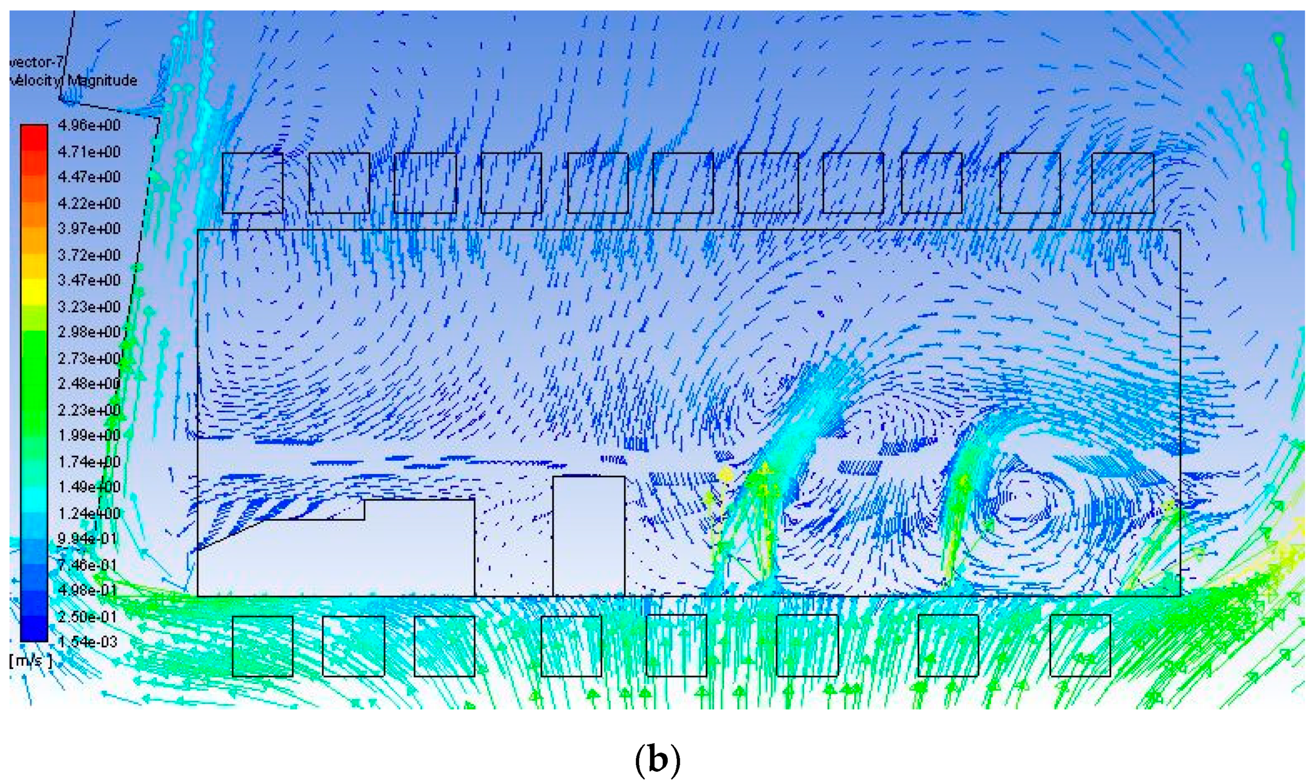
The study focused on the barn, so only the related results—and not the ones regard the context—will be discussed. The vortices were located in the North, South, and South-West of the barn, where there were several openings. Air velocity peaks were higher near the South-West openings, while the lowest air velocity values were detected in front of the office and between them (Figure 10 and Figure 11). The distribution of the air velocity well reflects the real conditions, where the internal distribution of the spaces and the position of the openings had a strong impact.
The data analysed were those regarding the areas considered more relevant for animal housing. In detail, average air velocity was equal to 0.42 ms−1 in the resting areas, service alley, and feeding alley, that housed dairy cows. With regard to box for calves, average air velocity was equal to 0.67 ms−1 (Figure 12).
4. Conclusions
The main objective of this study was to analyse the air velocity distribution inside a semi-open free stall barn, in order to
- Know the air velocity in areas considered most sensitive for the presence of animals;
- Find, in a future research based on the results of this study, alternative design configurations, with the aim to discover the best condition for the well-being of users and animals.
This objective was achieved in this study by developing a CFD model. Air velocity was measured in different indoor and outdoor points at different heights by using a Campbell system, with 15 min acquisition time. The 3D model was made by using Autodesk Autocad 2016®; then, it was imported into Ansys ICEM CFD 17.1® to build the unstructured mesh and to assign the boundary condition. Finally, the numerical simulations were carried out by using the Ansys-Fluent 17.1® program. A limitation not concerning the modelling process is that the experiment was conducted under isothermal cases. This choice, together with the simplification concerning the model, would not affect the objective of the present study, because for the authors all the elements that strongly affect the airflow development and air velocity distribution were taken into account, as reported in some past studies [2]. By using the described CFD methodology, a representation of the airflow distribution was given. It was considered good because it reflected the real condition inside the barn, where the internal distribution of the spaces and the position of the openings strongly impact the air velocity, and because of the comparison carried out between measured and simulated data. Therefore, the methodology applied in this paper could represent an example of how to study the natural ventilation of livestock buildings having similar characteristics. Since the modelled air velocity distribution in the barn fitted the real one well, the CFD model was considered reliable to study other transversal and longitudinal sections, by adding other anemometers. Future implementations should also regard the increase of the geometry complexity, or the study of gas distribution according to the study of airflow distribution. Furthermore, future studies will be carried out in order to evaluate the residence time of the air at each point of the model through the concept of “age of air”.
Author Contributions
Data curation, N.T. and F.V.; Funding acquisition, S.M.C.P.; Methodology, N.T.; Supervision, G.C.; Writing—original draft, N.T.; Writing—review & editing, S.M.C.P. and F.V..
Funding
This research was funded by University of Catania: UPB: 5A722192121 (Piano per la ricerca 2016-2018—progr. n.5 “Innovazioni attraverso applicazioni ICT nel settore delle Costruzioni Rurali, della Pianificazione del Territorio Agro-forestale e della Meccanizzazione della Difesa Fitosanitaria”).
Conflicts of Interest
The authors declare no conflict of interest.
References
- Shen, X.; Zhang, G.; Wu, W.; Bjerg, B. Model-based control of natural ventilation in dairy buildings. Comput. Electron. Agric. 2013, 94, 47–57. [Google Scholar] [CrossRef]
- Rong, L.; Bjerg, B.; Batzanas, T.; Zhang, G. Mechanisms of natural ventilation in livestock buildings: Perspectives on past achievements and future challenges. Biosyst. Eng. 2016, 151, 200–217. [Google Scholar] [CrossRef]
- Zhiqiang, Z.; Mankibib, M.; Zoubirb, A. Review of natural ventilation models. Energy Procedia 2015, 78, 2700–2705. [Google Scholar]
- Wathes, C.M.; Charles, D.R. Air and Surface Hygiene. Livestock Housing; CAB International: Wallingford, OX, USA, 1994; pp. 123–148. [Google Scholar]
- Zhang, Y. Engineering control of dust in animal facilities. In Proceedings of the Dust Control in Animal Production Facilities, Proc. Congress, Aarhus, Denmark, 30 May–2 June 1999. [Google Scholar]
- Allocca, C.; Chen, Q.; Glicksman, L.R. Design analysis of single-sided natural ventilation. Energy Build. 2003, 35, 785–795. [Google Scholar] [CrossRef]
- Bournet, P.E.; Boulard, T. Effect of ventilator configuration on the distributed climate of greenhouses: A review of experimental and CFD studies. Comput. Electron. Agric. 2010, 94, 47–57. [Google Scholar] [CrossRef]
- Bjerg, B.; Cascone, G.; Lee, I.; Bartzanas, T.; Norton, T.; Hong, S.; Seo, I.; Banhazi, T.; Liberati, P.; Marucci, A.; et al. Modelling of ammonia emissions from naturally ventilated livestock buildings. Part 3: CFD modelling. Biosyst. Eng. 2013, 116, 259–275. [Google Scholar] [CrossRef]
- Down, M.J.; Foster, M.P.; McMahon, T.A. Experimental verification of a theory for ventilation of livestock buildings by natural convection. J. Agric. Eng. Res. 1990, 45, 269–279. [Google Scholar] [CrossRef]
- Bruce, J.M. Wind tunnel study: Suckler cow building. Farm Build. Prog. 1974, 38, 15–17. [Google Scholar]
- Bruce, J.M. Natural Ventilation-Its Role and Application in the Bio-Climatic Systems; Farm Building R&D Studies; Scottish Farm Buildings Investigation Unit: Aberdeen, Scotland, 1977. [Google Scholar]
- Bruce, J.M. Natural convection through openings and its application to cattle building ventilation. J. Agric. Eng. Res. 1978, 23, 151–167. [Google Scholar] [CrossRef]
- Bruce, J.M. Ventilation of a model livestock building by thermal buoyancy. Trans. Am. Soc. Agric. Eng. 1982, 25, 1724–1726. [Google Scholar] [CrossRef]
- Foster, M.P.; Down, M.J. Ventilation of livestock buildings by natural convection. J. Agric. Eng. Res. 1987, 37, 1–13. [Google Scholar] [CrossRef]
- Gürdil, G.A.K. Numerical simulation of natural ventilation rates in laying hen houses. J. Anim. Vet. Adv. 2009, 8, 624–629. [Google Scholar]
- Liberati, P.; Zappavigna, P.A. dynamic computer model for optimization of the internal climate in swine housing design. Trans. ASABE 2007, 50, 2179–2188. [Google Scholar] [CrossRef]
- Sapounas, A.; Dooren, H.J.C.; Smits, M.C.J. Natural Ventilation of Commercial Dairy Cow Houses: Simulating the Effect of Roof Shape Using CFD. In Proceedings of the 1st IS on CFD Applications in Agriculture, Valencia, Spain, 9–12 July 2012; pp. 221–228. [Google Scholar]
- Norton, T.; Grant, J.; Fallon, R.; Sun, D.W. Assessing the ventilation performance of a naturally ventilated livestock building with different eave opening conditions. Comput. Electron. Agric. 2010, 71, 7–21. [Google Scholar] [CrossRef]
- Seo, I.H.; Lee, I.B.; Moon, O.K.; Kim, H.T.; Hwang, H.S.; Hong, S.W.; Bitog, J.P.; Yoo, J.I.; Kwon, K.S.; Kim, Y.H.; et al. Improvement of the ventilation system of a naturally ventilated broiler house in the cold season using computational simulations. Biosyst. Eng. 2009, 104, 106–117. [Google Scholar] [CrossRef]
- Norton, T.; Grant, J.; Fallon, R.; Sun, D.W. Assessing the ventilation effectiveness of naturally ventilated livestock buildings under wind dominated conditions using computational fluid dynamics. Biosyst. Eng. 2009, 103, 78–99. [Google Scholar] [CrossRef]
- Wu, W.; Zhai, J.; Zhang, G.; Nielsen, P.V. Evaluation of methods for determining air exchange rate in a naturally ventilated dairy cattle building with large openings using computational fluid dynamics (CFD). Atmos. Environ. 2012, 63, 179–188. [Google Scholar] [CrossRef]
- Arcidiacono, C.; Porto, S.M.; Cascone, G. On ammonia concentrations in naturally ventilated dairy houses located in Sicily. Agric. Eng. Int. CIGR J. 2015, 294–309. [Google Scholar]
- Arcidiacono, C.; D’emilio, A. CFD analysis as a tool to improve air motion knowledge in dairy houses. Riv. Ing. Agrar. 2006, 1, 35–42. [Google Scholar]
- VDI 3783 Part 9. Environmental Meteorology—Prognostic Microscale Wind Field Models—Evaluation for Flow around Buildings and Obstacles; Beuth Verlag: Berlin, Germany, 2005.
- Franke, J.; Hellsten, A.; Schlünzen, H.; Carissimo, B. Best practice guideline for the CFD simulation of flows in the urban environment. In COST Action; European Cooperation in Science and Technology: Brussels, Belgium, 2007. [Google Scholar]
- Ramponi, R.; Blocken, B. CFD simulation of cross-ventilation for a generic isolated building: Impact of computational parameters. Build. Environ. 2012, 53, 34–48. [Google Scholar] [CrossRef]
- Di Sabatino, S.; Buccolieri, R.; Pulvirenti, B.; Britter, R. Simulations of pollutant dispersion within idealised. urban-type geometries with CFD and integral models. Atmos. Environ. 2007, 41, 8316–8329. [Google Scholar] [CrossRef]
- Horan, J.M.; Finn, D.P. Sensitivity of air change rates in a naturally ventilated atrium space subject to variations in external wind speed and direction. Energy Build. 2008, 40, 1577–1585. [Google Scholar] [CrossRef]
- Perén, J.I.; vah Hooff, T.; Leite, B.C.C.; Blocken, B. CFD analysis of cross-ventilation of a generic isolated building with asymmetric opening positions: Impact of roof angle and opening location. Build. Environ. 2015, 85, 263–276. [Google Scholar] [CrossRef] [Green Version]
- Montazeri, H.; Montazeri, F. CFD simulation of cross-ventilation in buildings using rooftop windcatchers: Impact of outlet openings. Renew. Energy 2018, 118, 502–520. [Google Scholar] [CrossRef]
- Gromke, C.; Buccolieri, R.; Di Sabatino, S.; Ruck, B. Dispersion study in a street canyon with tree planting by means of wind tunnel and numerical investigations-evaluation of CFD data with experimental data. Atmos. Environ. 2008, 42, 8640–8650. [Google Scholar] [CrossRef]
- Valenti, F.; Porto, S.; Tomasello, N.; Arcidiacono, C. Enhancing Heat Treatment Efficacy for Insect Pest Control: A Case Study of a CFD Application to Improve the Design and Structure of a Flour Mill. Buildings 2018, 8, 48. [Google Scholar] [CrossRef]
- Rong, L.; Nielsen, P.V.; Bjerg, B.; Zhang, G. Summary of best guidelines and validation of CFD modeling in livestock buildings to ensure prediction quality. Comput. Electron. Agric. 2016, 121, 180–190. [Google Scholar] [CrossRef]
- Norton, T.; Sun, D.W.; Grant, J.; Fallon, R.; Dodd, V. Applications of computational fluid dynamics (CFD) in the modelling and design of ventilation systems in the agricultural industry: A review. Bioresour. Technol. 2007, 98, 2386–2414. [Google Scholar] [CrossRef]
- Launder, B.E.; Spalding, D.B. The numerical computation of turbulent flows. Comput. Methods Appl. Mech. Eng. 1974, 3, 269–289. [Google Scholar] [CrossRef]
- Guo, L.; Maghirang, R.G. Numerical simulation of airflow and particle collection by vegetative barriers. Eng. Appl. Comput. Fluid Mech. 2012, 6, 110–122. [Google Scholar] [CrossRef]
- Barth, T.J.; Jespersen, D.C. The Design and Application of Upwind Schemes on Unstructured Meshes. In Proceedings of the AIAA 27th Aerospace Sciences Meeting, Reno, Nevada, 9–12 January 1989; Technical Report AIAA-89-0366; NASA Ames Research Center: Moffett Field, CA, USA, 1989. [Google Scholar]
- He, X.; Wang, J.; Guo, S.; Zhang, J.; Wei, B.; Sun, J.; Shu, S. Ventilation optimization of solar greenhouse with removable back walls based on CFD. Comput. Electron. Agric. 2018, 149, 16–25. [Google Scholar] [CrossRef]
- Dati SIAS. 2016. Available online: www.sias.regione.sicilia.it (accessed on 15 April 2018).
- Wieringa, J. Updating the Davenport roughness classification. J. Wind Eng. Ind. Aerodyn. 1992, 41, 357–358. [Google Scholar] [CrossRef]
- Sullivan, R.; Greeley, R. Comparison of aerodynamic roughness measured in a field experiment and in a wind tunnel simulation. J. Wind Eng. Ind. Aerodyn. 1993, 48, 25–50. [Google Scholar] [CrossRef]
- Schlichting, H. Boundary Layer Theory, 7th ed; McGraw-Hill: New York, NY, USA, 1979; pp. 578–595. [Google Scholar]
- Gan, C.; Salim, S. Numerical Analysis of Fluid-Structure Interaction between Wind Flow and Trees. In Proceedings of the World Congress on Engineering, London, UK, 2–4 July 2014. [Google Scholar]
- Jeanjean, A.P.R.; Hinchliffe, G.; McMullan, W.A.; Monks, P.S.; Leigh, R.J. A CFD study on the effectiveness of trees to disperse road traffic emissions at a city scale. Atmos. Environ. 2015, 120, 1–14. [Google Scholar] [CrossRef] [Green Version]
- Zhang, Z.; Zhang, W.; Zhai, Z.; Chen, Q. Evaluation of various turbulence models in predicting airflow and turbulence in enclosed environments by CFD: Part-2—Comparison with experimental data from literature. HVAC R Res. 2007, 13, 871–886. [Google Scholar] [CrossRef]
Figure 1.
Plan of the barn.

Figure 2.
Section of the barn.

Figure 3.
Windward façade.

Figure 4.
Surrounding trees and rural buildings.

Figure 5.
Boundary conditions assigned to the computational domain.

Figure 6.
(a) Prevailing air velocity in the reference week and (b) prevailing magnitude in the reference week.
Figure 6.
(a) Prevailing air velocity in the reference week and (b) prevailing magnitude in the reference week.

Figure 7.
(a) Downwind mesh comparison, (b) mesh comparison inside the barn, and (c) upwind mesh comparison.
Figure 7.
(a) Downwind mesh comparison, (b) mesh comparison inside the barn, and (c) upwind mesh comparison.

Figure 8.
Indoor average velocity comparison for the three meshes.

Figure 9.
Position of Plane A and Plan B.

Figure 10.
(a). Plane A—air velocity distribution (ms−1) and (b) Plane A—air velocity vectors distribution (ms−1).
Figure 10.
(a). Plane A—air velocity distribution (ms−1) and (b) Plane A—air velocity vectors distribution (ms−1).


Figure 11.
(a) Plane B-air velocity distribution (ms−1) and (b) Plane B-air velocity vectors distribution (ms−1).
Figure 11.
(a) Plane B-air velocity distribution (ms−1) and (b) Plane B-air velocity vectors distribution (ms−1).


Figure 12.
Plane B–average air velocity in relevant areas (ms−1).


Table 1.
Livestock farms for each province of Sicily (ISTAT, 2010).
| Sicilian Provinces | Number of Livestock Farms |
|---|---|
| Trapani | 170 |
| Palermo | 964 |
| Messina | 698 |
| Caltanissetta | 188 |
| Enna | 420 |
| Catania | 397 |
| Ragusa | 1472 |
| Syracuse | 569 |
Table 2.
Detail of livestock farms for each province of Sicily (ISTAT, 2010).
| Number of Livestock Farms | ||||
|---|---|---|---|---|
| Sicilian Provinces | Cattles and Buffaloes Housing | Pigs Housing | Laying Hens Housing | Broilers Housing |
| Trapani | 113 | 9 | 65 | 13 |
| Palermo | 813 | 47 | 139 | 25 |
| Messina | 458 | 143 | 191 | 30 |
| Caltanissetta | 164 | 6 | 28 | 2 |
| Enna | 394 | 21 | 16 | 3 |
| Catania | 303 | 48 | 91 | 29 |
| Ragusa | 1389 | 159 | 60 | 19 |
| Syracuse | 535 | 52 | 38 | 6 |
Table 3.
Data comparison between measurements and simulations.
| N. Simulation | Air Velocity at Weather Station (10 m height) (ms−1) | Air Velocity Outside the Barn (ms−1) (Sensor B) | Air velocity Inside the Barn (ms−1) (Sensor A) | ||||
|---|---|---|---|---|---|---|---|
| MEASURED | SIMULATED | RELATIVE ERROR % | MEASURED | SIMULATED | RELATIVE ERROR % | ||
| 1 (27/04-22:00) | 1.90 | 1.14 | 1.38 | 18.84 | 0.24 | 0.29 | 16.90 |
| 2 (28/04-02:00) | 2.90 | 1.83 | 2.08 | 13.02 | 0.40 | 0.45 | 12.31 |
| 3 (28/04-06:00) | 2.70 | 2.04 | 1.89 | 7.56 | 0.44 | 0.44 | 0.32 |
| 4 (28/04-07:00) | 2.70 | 1.96 | 1.89 | 3.64 | 0.46 | 0.44 | 5.00 |
| 5 (28/04-19:00) | 6.40 | 3.94 | 4.59 | 15.31 | 0.98 | 0.98 | 0.08 |
| 6 (28/04-20:00) | 6.00 | 3.43 | 4.31 | 22.82 | 0.79 | 0.91 | 14.70 |
| 7 (28/04-21:00) | 7.80 | 3.38 | 5.58 | 49.21 | 0.89 | 1.19 | 29.13 |
| 8 (28/04-22:00) | 7.90 | 4.51 | 5.66 | 22.65 | 1.07 | 1.20 | 11.36 |
| 9 (29/04-00:00) | 5.80 | 4.06 | 4.17 | 2.68 | 0.95 | 0.88 | 7.71 |
| 10(29/04-01:00) | 6.80 | 4.27 | 4.89 | 13.45 | 1.10 | 1.03 | 6.35 |
| 11(29/04-02:00) | 8.20 | 5.50 | 5.89 | 6.89 | 1.23 | 1.26 | 2.07 |
| 12(29/04-03:00) | 6.80 | 4.45 | 4.89 | 9.48 | 1.02 | 1.03 | 0.98 |
| 13(29/04-05:00 | 8.50 | 3.97 | 6.08 | 42.04 | 0.89 | 1.29 | 36.98 |
| 14(29/04-06:00) | 8.50 | 4.13 | 6.08 | 38.17 | 0.87 | 1.29 | 39.22 |
| 15(30/04-00:00) | 2.00 | 1.16 | 1.44 | 21.30 | 0.32 | 0.31 | 4.23 |
| 16(30/04-01:00) | 2.50 | 1.45 | 1.80 | 21.65 | 0.27 | 0.38 | 35.59 |
| 17(30/04-02:00) | 2.00 | 1.34 | 1.44 | 7.48 | 0.32 | 0.31 | 1.98 |
| 18(01/05-01:00) | 2.80 | 2.00 | 2.01 | 0.54 | 0.45 | 0.43 | 4.72 |
| 19(01/05-02:00) | 2.00 | 1.99 | 1.44 | 32.04 | 0.39 | 0.31 | 23.36 |
| 20(01/05-05:00) | 1.40 | 0.93 | 0.98 | 5.43 | 0.32 | 0.24 | 29.61 |
© 2019 by the authors. Licensee MDPI, Basel, Switzerland. This article is an open access article distributed under the terms and conditions of the Creative Commons Attribution (CC BY) license (http://creativecommons.org/licenses/by/4.0/).
Share and Cite
MDPI and ACS Style
Tomasello, N.; Valenti, F.; Cascone, G.; Porto, S.M.C. Development of a CFD Model to Simulate Natural Ventilation in a Semi-Open Free-Stall Barn for Dairy Cows. Buildings 2019, 9, 183. https://doi.org/10.3390/buildings9080183
AMA Style
Tomasello N, Valenti F, Cascone G, Porto SMC. Development of a CFD Model to Simulate Natural Ventilation in a Semi-Open Free-Stall Barn for Dairy Cows. Buildings. 2019; 9(8):183. https://doi.org/10.3390/buildings9080183
Chicago/Turabian StyleTomasello, Nicoletta, Francesca Valenti, Giovanni Cascone, and Simona M. C. Porto. 2019. "Development of a CFD Model to Simulate Natural Ventilation in a Semi-Open Free-Stall Barn for Dairy Cows" Buildings 9, no. 8: 183. https://doi.org/10.3390/buildings9080183
Note that from the first issue of 2016, this journal uses article numbers instead of page numbers. See further details here.