How Eudaimonic Aspect of Subjective Well-Being Affect Transport Mode Choice? The Case of Thessaloniki, Greece


Department of Transportation and Hydraulic Engineering, School of Rural and Surveying Engineering, Faculty of Engineering, Aristotle University of Thessaloniki, Thessaloniki 54124, Greece
*
Author to whom correspondence should be addressed.
Soc. Sci. 2019, 8(1), 9; https://doi.org/10.3390/socsci8010009
Submission received: 28 November 2018
/
Revised: 24 December 2018
/
Accepted: 27 December 2018
/
Published: 7 January 2019
(This article belongs to the Special Issue Public Transport and Social Psychology)
Abstract
:In recent years, the relationship between transportation and subjective well-being has been a major subject. Well-being is a factor that can affect travelers’ psychology and transport mode choice. For this reason, policymakers have attempted to improve travelers’ subjective well-being and promote sustainable modes of transport. For a better understanding of these factors, a questionnaire-based survey was conducted to identify the travel eudaimonia aspect of subjective well-being (comfort, safety, autonomy, self-confidence, physical, and mental health), for the various means of transport in the city of Thessaloniki. During the survey, 300 valid questionnaires were completed. The collection of the above data was followed by statistical analysis. The aim of the analysis was to identify the factors of travel eudaimonia that contributed to the mode choice. For that reason, four ordinal regression models were developed to determine how travel eudaimonia affected the usage frequency of the four available means of transport in the city of Thessaloniki (i.e., private car, bicycle, public transport, walking). Walking was rated higher than other modes in all factors, whilst cycling was rated high in physical and mental health, self-confidence, and autonomy, but low in comfort and safety. Public transport scored very low in all factors, demonstrating the poor quality of service provided by the city’s public transport. Moreover, from the ordinal regression models’ results, it could be demonstrated that travel eudaimonia factors had a significant role to play in mode choice. Recognizing the impact of these factors on transport mode choice is particularly useful for policymakers, researchers, and engineers, as it helps them to make informed decisions about what improvements are needed to promote sustainable modes of transport (mainly walking, cycling, and secondarily, public transport).
1. Introduction
Mode choice or modal split is an important stage in the transport planning process, and it is very useful for policymakers (Minal and Sekhar 2014). Transport mode choice is currently exercised by means of discrete choice models (Ben-Akiva and Lerman 1985). In these models, the available alternatives are exclusive and collectively exhaustive (Koppelman and Bhat 2006). Discrete models are based on selecting the alternative that provides the highest utility to the choice maker. There are plenty of unobservable and situational variables that make this decision complicated (Koppelman and Bhat 2006). For this reason, random utility theory was developed (Mcfadden 1980).
Utility is an indicator of value to an individual (Koppelman and Bhat 2006). An individual selects a mode of transport which maximizes the individual’s utility (Khan 2007). This theory is known as utility maximization. Random utility models consist of two components. The first component of the utility function is the deterministic part of the utility that is observed by the analyst (Minal and Sekhar 2014). The second component is the difference between the unknown utility of each individual and the observed one (Minal and Sekhar 2014). Discrete choice models, which are based on maximizing random utility, are widely used in transport applications (Francois et al. 2017).
One of the important issues in mode choice modelling relates to the factors that explain the trip makers’ mode choice. Mode choice is influenced by a plethora of social, economic, cultural, and environmental factors (Minal and Sekhar 2014). Additionally, the socio-economic characteristics of the trip maker, such as the household income, gender, age, employment, car ownership, social status, and the number of people in the household, have an important role in the mode choice (de Dios Ortúzar and Willumsen 2011). Two other influencing factors are the trip purpose and the relative cost of the modes of transport in relation to the service that they provide (Giannopoulos 2005). The parameters that affect this selection and are related to the mode of transport include travel time, cost, waiting time, in-vehicle time, walking time, comfort, safety, security, etc., (de Dios Ortúzar and Willumsen 2011). Therefore, mode choice models deal with the range of trade-offs that individuals are willing to make amongst these factors (Ben-Akiva and Lerman 1985; Koppelman and Wen 2000). In a more recent study, it was observed that trip characteristics could affect mode choice (Racca and Ratledge 2004).
2. Literature Review
One of the most important factors influencing the mode choice is the value of travel time. Value of time is the extra cost the passenger would like to pay to avoid increasing the travel time while using a typical mode of transport (Minal and Sekhar 2014). In addition to all these factors, the psychology of the trip maker plays a significant role in the mode choice. For mandatory trips (e.g., work, education), travel time is a disutility that people seeking to minimize. Nevertheless, in some cases, trips are made not to reach a destination but rather for relaxation, exercise, and entertainment from the trip itself. As a result, the trip makers are seeking to maximize the satisfaction and joy of the trip, rather than minimizing the disutility (Singleton 2017).
The idea that a trip can provide benefits without reaching a destination is known as the “positive utility of travel”. This concept indicates that travelers can have positive emotions for traveling itself, regardless of the benefits that derive from the activities that they can engage in at the destination. This concept was originated by Mokhtarian and Salomon (2001), and it was followed by many studies. The positive utility of travel idea assembles several concepts of the travel behavior field: Utility maximization (McFadden 2001), motivation theory (Ryan and Deci 2000), and multi-tasking (Kenyon 2010), amongst others. Consequently, the positive utility of travel can be defined as “any benefit accruing by a traveler through the act of traveling” (Singleton 2017). This concept could also be divided into the following three categories:
- Destination activities;
- Travel activities;
- Travel experience (Mokhtarian and Salomon 2001; Singleton 2017).
More specifically, destination activities refer to all the benefits that a traveler will gain from the activities he/she will engage in at the destination if he/she deducts the generalized cost (i.e., cost and travel time) of reaching the destination (Singleton 2017). Travel activities refer to all the activities that a trip maker can perform whilst traveling. Most of the activities that a person performs daily can also be carried out during his or her trip, such as talking, eating, reading, sleeping, listening to music, etc. There are many researches concerning these activities (Mokhtarian et al. 2015). Finally, the travel experience refers mainly to the benefits that travelers can have from the experience of traveling (Singleton 2017).
Other researches examine the experience of traveling only, where travel is intrinsically motivated by positive sensations, emotions, and purposes. Many of the intrinsic motivations related to the travel experience are founded in the psychological conceptualizations of subjective well-being (Singleton 2017). Consequently, travel experience is related to subjective well-being (Singleton 2017). Subjective well-being is a concept with multiple dimensions, including health, satisfaction, happiness, and quality of life (Nordbakke and Schwanen 2014). Subjective well-being is defined as ‘a broad category of phenomena that includes people’s emotional responses, domain satisfactions and global judgments of life satisfaction’ (Diener et al. 1999). Additionally, subjective well-being is related to peoples’ individual perception and experience (Singleton 2017). Transportation and subjective well-being are closely linked. Many reviews have summarized the evidence of the effect of transportation on well-being (Delbosc 2012). Subjective well-being can be decomposed into two basic aspects: Hedonic and eudaimonic. Hedonic is related to satisfaction, utility, and the feelings of happiness, while the eudaimonic is related to the meaning of life, personal growth, achievement of goals, and self-realization (De Vos et al. 2013). Thus, hedonic is related to the enjoyment of the traveling experience, whilst eudaimonic is related to positive psychology from the travel experience (Singleton 2017).
There are a series of established scales that have been carried out for the measurement of subjective well-being through various researches (Ettema et al. 2010; De Vos et al. 2013). The concept of “Satisfaction with travel scale” was also developed to measure the hedonic aspect of subjective well-being (Ettema et al. 2011). This concept has been used for research in many cases, such as leisure trips, commute, etc. (De Vos et al. 2015; Ettema et al. 2012). According to Olsson et al. (2013), active modes of transport provide higher levels of travel satisfaction compared to car, and especially public transport. Moreover, it has been observed that commuting has a less positive value than other types of trips (Ory and Mokhtarian 2005). Far fewer studies have dealt with the eudaimonic aspect of subjective well-being due to the difficulty of measuring these characteristics in the transport sector (Singleton 2018). A case study in Shanghai indicates that the development of rail transit and transit-oriented development can increase happiness (well-being) (Li et al. 2018). The impact of eudaimonia in tourism has also been examined in another study, which found that many tourists’ best experiences in various contexts were linked to eudaimonia (Knobloch et al. 2017). This study aimed at assisting decision making in tourism, whilst there were also other methods, for instance, using location-based marketing apps, which could also contribute in this direction (Palos-Sanchez et al. 2018).
Few studies have been carried out concerning the relationship between subjective well-being and the positive utility of travel with mode choice. Studies that have been carried out in that field suggest that there may be a link between the increase in positive feelings or subjective well-being with mode choice (Gardner and Abraham 2007; Singleton 2018). Studies of attitudes and non-instrumental motivations for car use suggest that the enjoyment of driving might render people more likely to drive (Gardner and Abraham 2007). In fact, a stated preference survey suggests that people who consider happiness from travel as an important parameter were more likely to drive than to use public transport (Duarte et al. 2010). Travelers are also likely to change their travel behavior (i.e., mode or route choice) to improve their well-being (Abou-zeid and Ben-Akiva 2012; Abou-zeid and Ben-Akiva 2014).
In this study, an empirical effort was made to measure the eudaimonic aspects of subjective well-being, and their relation to the mode choice in the city of Thessaloniki, Greece. The aim was to identify which travel eudaimonia aspects (comfort, safety, autonomy, self-confidence, physical, and mental health) (Singleton 2018) contributed to travelers’ choice amongst the four available modes of transport in the city (private car, bicycle, public transport, walking). Moreover, we attempted to quantify the impact of the travel eudaimonia aspects on the usage frequency of the four modes.
3. Materials and Methods
The research hypothesis of this paper was that beyond the travel cost and travel time, which are mainly taken into consideration by researchers and engineers, there were other factors that were related to travelers’ psychology and that influenced the transport mode choice. One factor that affects a traveler’s phycology is the eudaimonic aspect of subjective well-being.
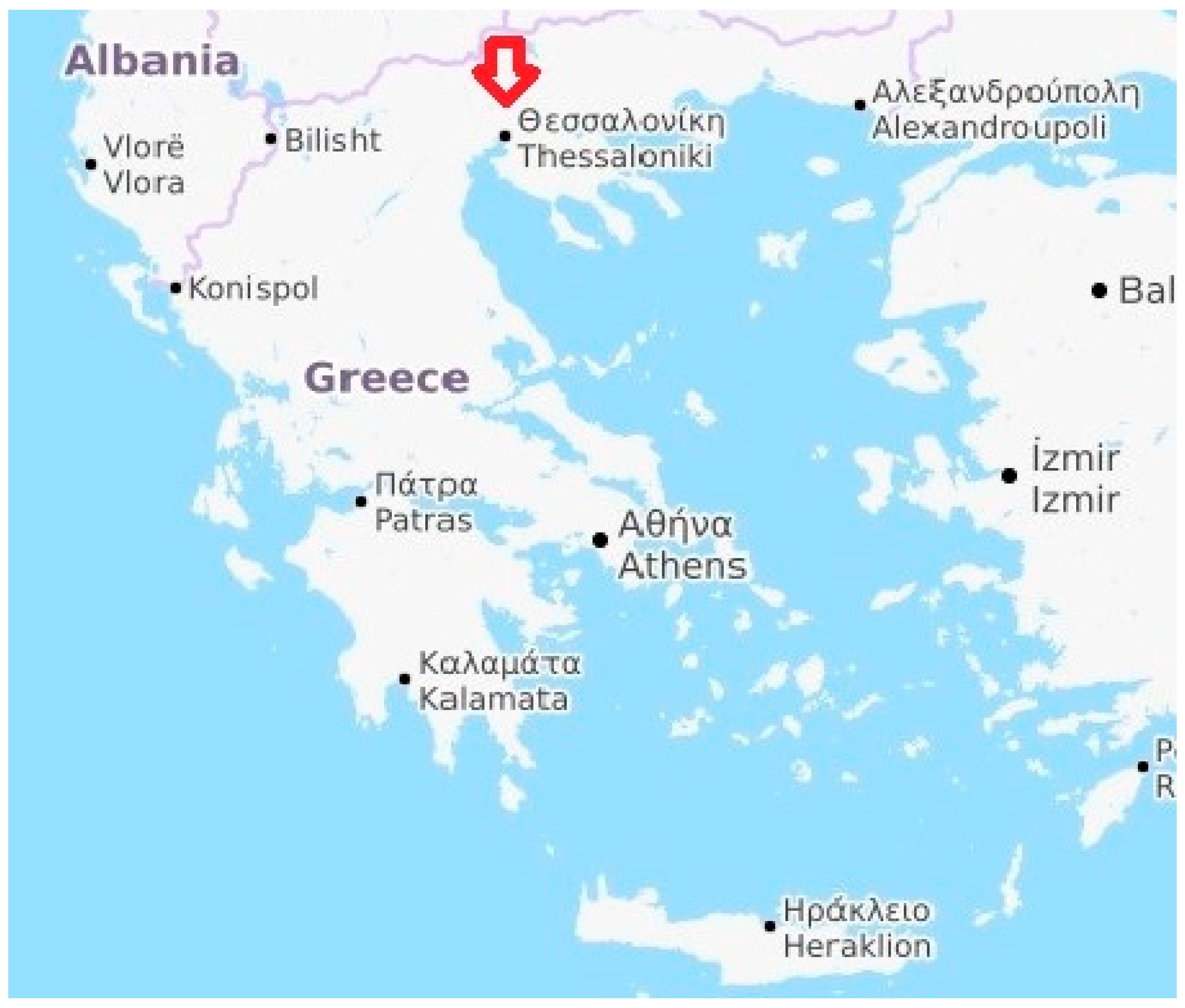
To investigate the relation between the eudaimonic aspect of subjective well-being and mode choice in the city of Thessaloniki, a questionnaire-based survey was designed and addressed to the residents of Thessaloniki. Thessaloniki is the second largest city in Greece, with a population of 1,006,730 people in its greater area, and it is a major Greek harbor and university center (ELSTAT 2011). The tourism sector of the city continues to develop, where the number of overnight stays in 2017 grew by 2.7 percent to 2,371,905 compared to 2,309,617 in 2016 (Thessaloniki Hotels Association 2017). Figure 1 presents a map of Greece and it highlights the position of Thessaloniki.
In this point, some key facts about the transport system of Thessaloniki must be mentioned. According to a case study, the majority of trips in Thessaloniki were conducted using private cars (67%), while 23% were conducted using public transport, and 2% using non-motorized modes of transport (Mitsakis et al. 2013). The bicycle lanes total length is 11.73 km and these lanes do not form a coherent network that provides sufficient accessibility to the cyclists. For this reason, the built environment is not so safe and comfortable for cyclists. As far as public transport is concerned, there is no metro or tram system in the city. Public transport trips are carried out using only buses. During peak hours, the buses operate in saturation conditions and that is a major problem, which demotes the quality of service provided by the public transport. It is necessary to promote more sustainable modes in the city due to the existence of air pollution and pollutants from the transport system (Nikolaou et al. 2002; Basbas et al. 2004). Some case studies have investigated this problem (Nikolaou et al. 2004; Basbas et al. 2001).
Firstly, a questionnaire was structured and modified slightly after the implementation of a pilot survey, which was conducted on the 4th of July 2018. During the pilot survey, 10 questionnaires were completed, and they were not included in the final sample. The study employed face-to-face interviews to achieve a high response rate and better quality of data. The final survey took place from the 20th of July until the 10th of August in the busy pedestrian streets in the center of the city. During the survey, 300 questionnaires were completed by passing pedestrians in the above locations and were considered as valid.
The questionnaire itself consisted of 35 questions allocated across three sections. The first section contained six questions regarding the socio-economic characteristics of the respondent, such as gender, age, education level, household income, car ownership, and bike ownership. The second section contained five questions, which were related to the usage of the under-consideration means of transport (i.e., private car, bicycle, public transport, walking). The last section of the questionnaire contained the remaining 24 questions, which were related to the assessment of the travel eudaimonia factors by the respondents, for each of the four modes of transport. For the assessment of the travel eudaimonia factors, the 5-point Likert scale was used (Likert 1932).
The collection of the above data was followed by statistical analysis. At first, a descriptive statistical analysis was conducted to understand the socio-economic characteristics of the respondents, the usage frequency of the means of transport, and the assessment of travel the eudaimonia factors for each mode.
To meet the objective of this study, four ordinal regression models were developed based on the questionnaire survey. Ordinal logistic regression is a type of statistical model used when the dependent variable is of an ordinal nature (see Gutiérrez et al. 2016 for more details). The motivation to develop such models was the shift towards sustainable mobility taking place in many countries. Using these models, we attempted to identify the factors that could increase the usage frequency of sustainable transport modes. Thus, the statistical analysis and the ordinal regression models could represent an important aid for transport and urban planners globally, especially in cities with characteristics that are similar to Thessaloniki. The dependent variable for the models was the usage frequency of the respective transport mode, and the independent variables comprised a combination of socio-economic characteristics and travel eudaimonia factors.
4. Descriptive Statistics
The main outcomes derived from the descriptive statistical analysis of this paper are presented in this section. Appendix A presents the coding of the variables, the measurement scale, and the results of the descriptive statistics. It should be noted that the entire statistical analysis was carried out using the SPSS v23.0 software.
Most of the participants in the survey were male (57.3%). Most of the respondents were between 25–39 years old (48%), while the other age groups had a lower participation, especially the elderly (65+). Additionally, most of the respondents (29%) had an 800–1200 € monthly household income and their level of education was high (at least a bachelor’s degree). Car ownership in the households was extremely high (76%), whilst bicycle ownership was around 40%.
Private car daily usage for at least one trip had a high percentage rate. This result agreed with the modal split of Thessaloniki (Mitsakis et al. 2013). Moreover, the usage frequency of the bicycle was very low due to the problems mentioned above regarding the bicycle networks in the city. Public transport was used daily at a rate of 22%, and most of the users were captive users of public transport. Trips on foot for distances longer than 10 min had very high rates. This result may have been due to the distances that car drivers had to make from the car parking to the place that they sought to finally reach or for the entertainment and exercise. Finally, the respondents sought to more frequently use a bicycle or private car, but they did not use these modes due to the lack of safety or parking, respectively.
The private car was rated high in all travel eudaimonia factors. The only factor where the private car was rated lower relative to the others was safety. Cycling was rated high in physical and mental health, self-confidence, and autonomy; however, it was rated low in comfort and safety. In these two factors, the bicycle was rated much lower than the other modes of transport, and therefore, it was understood that additional efforts should be made to promote cycling in cities with a low cycling experience, such as Thessaloniki. Public transport was rated low in all factors, demonstrating the poor quality of service, mostly in peak hours. The only factor where public transport had more positive responses than negative was safety, due to the lack of accidents by buses in the city. Finally, walking was rated much higher than the others means of transport in all factors. This was a fact that agreed with the results of other studies (Singleton 2018).
5. Development of the Ordinal Regression Models
In this section, four ordinal regression models were developed to investigate the travel eudaimonia factors which influenced the usage frequency of the four available means of transport in Thessaloniki. In every model, the dependent variable was the usage frequency of the respective mode of transport.
The independent variables for these models included a combination between the socio-economic characteristics of the respondents and the travel eudaimonia factors, based on the data which was obtained from the questionnaire survey. SPSS software was used to develop the models. Given that this software automatically uses the last class as a reference category when applying an ordinal regression, it was necessary to re-code the independent variables, so that the reference category collected many responses. Appendix B presents the independent variables and the parameter estimates for each of the developed models. Parameter estimate tables contain the parameter (beta) estimates, the standard error, the Wald statistics, and the significance level, amongst others.
5.1. Model 1: Private Car Usage Frequency
In this model, the dependent variable was the usage frequency of the private car. Gender, age, and the assessment of safety by the car driver were independent variables included in the model.
Before proceeding with the interpretation of the model, it was important to present the overall fitting indices of the model, which can be found in Table 1. It could be observed from the first section of Table 1 (Model Fitting Information) that the sig. was lower than 0.05, which led to the conclusion that the explanatory coefficients improved the model, compared to the baseline (intercept only) model without the independent variables. Additionally, by observing the part of the table that referred to “goodness-of-fit,” we concluded that the model had a good fit, since sig > 0.05 (the null hypothesis was that the fit was good). The Nagelkerke R-Square suggested that the final model could explain 21.1% of the variance of the dependent variable. Finally, the test of parallel lines showed that the null hypothesis was rejected, and therefore, the relation between the dependent variable’s thresholds and the explanatory variables was the same for all the thresholds.
The interpretation of the ordinal regression models was based on the calculation of the odds ratios. Table 2 presents the odds ratios of the private car model. It should be noted that in the table, we only showed the odds ratios of the classes of independent variables that were statistically significant.
From Table 2, useful conclusions can be noted. Males were more likely to use the private car more frequently than females. The age group 18–24, which was referred to as young people, were more likely to use the private car less frequently than the other classes because they either had no car or they were not the main user of the vehicle. People aged between 40 and 54 were approximately six times more likely to use a private car than people aged between 18 and 24. Regarding the travel eudaimonia factors, only safety participated in the model. The respondents that were absolutely satisfied with the safety that a private car provided were more likely to use it more often.
5.2. Model 2: Bicycle Usage Frequency
The second model had bicycle usage frequency as the dependent variable. Monthly household income and the assessment of self-confidence by the cyclist were the only independent variables in this model.
Table 3 presents the overall fitting indices of the statistical model for the bicycle usage frequency. The model fitting information indicated that the explanatory coefficients improved the model, hence the sig < 0.05. From the second part of the table, it was concluded that the model had a good fit, since the sig was greater than 0.05. From the next section of the table (Nagelkerke R-Square), it was observed that the final model could only explain 8.1% of the variance of the dependent variable. This result was because most of the respondents did not ride a bicycle at all, so the distribution of the answers was extremely uneven. Finally, the test of parallel lines showed that the null hypothesis was not rejected in this model, and therefore, the relation between the dependent variable’s thresholds and the explanatory variables was not the same for all the thresholds. According to O’Connell (2006), using this test, in most cases the result leads to the rejection of the proportional odds assumption. For this reason, this model was accepted by the researchers.
Table 4 presents the odds ratios of the bicycle model. This table contained only the odds ratios of the classes of independent variables that were statistically significant.
The model contained two independent variables, the first variable was monthly household income and the second variable was self-confidence. People with high income were more likely to use the bicycle more frequently than all the other classes with lower income. As the income decreased, the likelihood was to reduce the usage frequency of the bicycle. Concerning the self-confidence assessment by the cyclist, it was concluded that respondents that were absolutely satisfied were more likely to use the bicycle more often than the other classes of this independent variable.
5.3. Model 3: Public Transport Usage Frequency
In this model, the dependent variable was public transport usage frequency. Gender, age, and the assessment of comfort by the public transport users were included in the model as the statistically significant independent variables.
Table 5 presents the overall fitting indices of the public transport model. From the first section of the table (Model Fitting Information), it was noted that the explanatory coefficients improved the model compared to the baseline model without the independent variables. Additionally, the second part concluded that the model had a good fit due to the rejection of the null hypothesis. From the third part of the table (Pseudo R-Square), we deduced that the model explained about 30% of the relative variance of the dependent variable. Finally, the test of parallel lines showed that the zero hypothesis was rejected, and therefore, the relation between the dependent variable’s thresholds and the explanatory variables was the same for all the thresholds.
Table 6 presents the odds ratios of the independent variables. The table only contained the statistically significant classes of the independent variables. Males were less likely to use public transport than females. Additionally, the 18–24 age group was more likely to frequently use the public transport system of the city compared to the other age groups. Important to note that the 40–54 age group was opposed to using public transport, and it was 15 times more likely to not use this mode of transport compared to the reference category (age 18–24). Concerning the travel eudaimonia factors, only comfort was found as significant. The respondents that were not satisfied with the comfort that public transport provided, were less likely to use it than all the other classes.
5.4. Model 4: Walking Frequency
The last model used walking frequency as the dependent variable. The independent variables for the model were age, monthly household income, and the assessment of safety and self-confidence by the pedestrian.
Before proceeding with the interpretation of the model, it was important to analyze the overall fitting indices of the model. The overall fitting indices of making trips on foot are presented in Table 7. The model fitting information indicated that the explanatory coefficients improved the model compared to a baseline model without the independent variables. From the second part of the table, it could be concluded that the model had a good fit. Observing the Nagelkerke R-Square suggested that the model explained 18.3% of the dependent variable’s variance. Finally, the test of parallel lines showed that the relation between the dependent variable’s thresholds and the explanatory variables was the same for all the thresholds.
The last model had four independent variables and useful conclusions could be derived from it. The 18–24 age group was more likely to travel on foot compared to all the other classes. However, the odds ratios of all the classes were too close to the value 1, which meant that the other classes also often used walking for their trips. The respondents with a low monthly household income were more likely to walk to make a trip than the higher income classes. Regarding the travel eudaimonia factors, it could be concluded that the respondents who perceived high levels of safety and self-confidence while walking, were more likely to walk frequently. The high values for safety and self-confidence in Table 8 indicated that these travel eudaimonia factors were one of the most decisive factors for making trips on foot.
6. Discussion
Predicting travelers’ mode choice is very important in transport planning. While most studies focus on the cost and time parameters, there appear to be many other factors that influence mode choice. One of these factors is subjective well-being. Few studies have been carried out concerning the relationship between subjective well-being and the mode choice. Even fewer studies have dealt with the eudaimonic aspect of subjective well-being, and how it can affect the daily mode choice. Through this study, we attempted to quantify the impact of the travel eudaimonia aspects on the usage frequency of four transport modes (private car, public transport, bicycle, walking). For that reason, four ordinal regression models were developed to identify which travel eudaimonia factors in combination with socio-economic characteristics affected the usage frequency of the means of transport under consideration.
From descriptive statistics useful conclusions could be extracted. The private car was being used daily at a 40% rate, although 76% of the respondents had a private car in their household. Consequently, it was concluded that these respondents were not the main users of the private car or that they did not use the car for other reasons, such as the lack of parking spaces in the city center. Daily usage of the bicycle was very low due to the deficiencies and problems identified in the existing network. Public transport usage frequency agreed with the modal split of the city (22%). Most of the users of public transport were captive, as they did not have access to a private car. Finally, trips on foot had the highest rates amongst the various means of transport in Thessaloniki.
Concerning the travel eudaimonia, it is important to note the most useful findings. The private car was rated highly in all travel eudaimonia factors. Safety and autonomy of the private car were rated a bit lower than the other factors, because the respondents took the lack of parking space into account in terms of autonomy. The bicycle was rated highly in all factors, except comfort and safety, due to the insufficient cycling infrastructure, as already mentioned. Public transport was rated low in all factors because of the saturation phenomena observed during peak hours, which downgraded the quality of service provided by the public transport system. Finally, walking was rated highly in all factors and this conclusion agreed with results by Singleton (2018). According to Duarte et al. (2010), cycling and walking are the two modes of transport which provide the highest levels of happiness to the trip makers during their mandatory trips. This finding largely agrees with the results of the Olsson et al. (2013) study.
From the four developed models, we observed that travel eudaimonia factors had a significant impact on the usage frequency of the available modes of transport in Thessaloniki. More specifically, comfort, safety, and self-confidence were found to have a significant influence on mode choice. Safety was the factor that influenced private car usage frequency, because when travelers feel more protected during their trip, they increase the usage frequency. Bicycle usage frequency increased with the increase in self-confidence of the cyclist. Comfort was the factor that influenced public transport usage the most. Given the problems of saturation during peak hours, the improvement of comfort may increase the usage frequency of public transport. Finally, walking was influenced by safety and self-confidence more significantly than the socio-economic characteristics. It could be observed from the odds ratio table that safety significantly influenced the mode choice. Respondents who were unsatisfied with the safety of making trips on foot were about 16 times less likely to travel in that way. The safer people that felt when traveling on foot in the city, the higher the demand for making trips on foot. The same applied for self-confidence to an even greater extent, since the odds ratio value was about 232.
Overall, it can be concluded that travel eudaimonia factors are an important parameter that influences mode choice in the city of Thessaloniki. Additionally, public transport and the bicycle, which provide the opportunity to travel at low-cost and in a relatively shorter time, were not preferred by its citizens. This was because of: (a) The insufficient cycling infrastructure, which created an unfriendly environment for cyclists; and (b) The lack of other means of public transport (e.g., metro, tram), resulting in the operation of public transport at levels of saturation in the current situation.
7. Conclusions
It seems that subjective well-being is an extremely important factor that people consider when making decisions about their daily trips. The results from Thessaloniki reinforced the findings of other surveys on the fact that walking and cycling were two modes of transport that contributed to the travelers eudaimonia. For this reason, as well as for social benefits, many efforts have been made in recent years to promote these two transport modes. However, especially for the bicycle, it seems that extra action is needed in cities with little experience and tradition in cycling, such as Thessaloniki, where trips with bicycle were assessed as “very low” in terms of comfort and safety. In addition, the results of this paper reinforce the views expressed in other papers that well-being factors are a parameter influencing the transport mode choice. The results also demonstrate that safety is an important factor that influences transport mode choice. Moreover, great impression creates the fact that confidence has significant contribution in two models Comfort also plays a significant role in travelers’ decisions to use public transport. It seems that the low quality of service, which public transport provides according to the passengers, makes comfort an important factor in their choice. On the other hand, autonomy, physical health, and mental health were the three travel eudaimonia aspects that did not appear to have a significant impact on the transport mode choice. These results may assist policy makers, researchers, and engineers to make sound decisions to improve the appropriate factors, with the ultimate goal of strengthening the means of transport that local policy seeks to promote.
The data collection was carried out in Thessaloniki, where the cycling levels were very low due to the underdeveloped bicycle infrastructure network, and public transport also provided insufficient services as perceived by the passengers. Consequently, this fact represents a limitation of the survey, since the results could be significantly different in cities which are characterized as established cycling cities or in cities which provide high quality public transport services. Especially for the bicycle, the low levels of usage do not allow the extraction of sound conclusions from the bicycle model. Another limitation of the survey was that the data was collected during summer. Even though respondents were not asked about the trip they were making at the time of the interview, in a more frequent situation, they might have been affected by the conditions prevailing at that time.
Future research includes the development of statistical models using other techniques (e.g., mixed logit models), also considering the travel time and cost as independent variables to identify the importance of travel eudaimonia compared to these two variables. Finally, it would be very interesting to explore how travel eudaimonia factors affect the route choice in addition to mode choice.
Author Contributions
Conceptualization, S.B. and A.N.; Data curation, P.V.; Investigation, P.V.; Methodology, S.B. and A.N.; Supervision, S.B.; Writing—original draft, P.V.; Writing—review & editing, P.V. and A.N.
Funding
This research received no external funding.
Acknowledgements
The authors would like to thank the anonymous reviewers and the editor for their suggestions in order to improve the manuscript.
Conflicts of Interest
The authors declare no conflict of interest.
Appendix A

Table A1.
Coding and descriptive statistics of the variables used in the study.
| Code | Explanation | Values | Frequency (%) |
|---|---|---|---|
| gender | Gender | 0: male, 1: female | 0: 57.3, 1: 42.7 |
| age | Age | 0: 18–24, 1: 25–39, 2: 40–54, 3: 55–64, 4: ≥65 | 0: 19.66, 1: 47.66 2: 21.66, 3: 7, 4: 4 |
| income | Monthly household income | 0: 0–400, 1: 401–800, 2: 801–1200, 3: 1201–1600, 4: 1601–2000, 5: >2000 | 0: 13.66, 1: 15.66, 2: 29.33, 3: 16, 4: 10.66, 5: 14.66 |
| education | Level of education | 0: Primary school, 1: secondary school, 2: high school,3: undergraduate student, 4: bachelor, 5: master/PhD | 0: 1.33, 1: 3.33, 2: 23.66, 3: 12.33, 4: 38, 5: 21.33 |
| carhold | Car ownership | 0: yes, 1: no | 0: 76, 1: 24 |
| bikehold | Bicycle ownership | 0: yes, 1: no | 0: 40.3, 1: 59.7 |
| cardriver | Private car usage frequency (as a driver) | 0: more than 1 a day, 1: 1 a day, 2: 2–3 times in week, 3: 1 in week, 4: rarely, 5: not at all | 0: 28, 1: 11.67, 2: 16.33, 3: 6, 4: 7.33, 5: 30.67 |
| bikeuse | Bicycle usage frequency | 0: more than 1 a day, 1: 1 a day, 2: 2–3 times in week, 3: 1 in week, 4: rarely, 5: not at all | 0: 2.67, 1: 0.67, 2: 5.67, 3: 4.33, 4: 15.67, 5: 71 |
| ptranspuse | Public transport usage frequency | 0: more than 1 a day, 1: 1 a day, 2: 2–3 times in week, 3: 1 in week, 4: rarely, 5: not at all | 0: 22, 1: 9.33, 2: 12, 3: 8.67, 4: 17, 5: 31 |
| walkuse | Frequency of making trips on foot | 0: more than 1 a day, 1: 1 a day, 2: 2–3 times in week, 3: 1 in week, 4: rarely, 5: not at all | 0: 52, 1: 19, 2: 16.33, 3: 6.33, 4: 3.67, 5: 2.67 |
| othermode | Mode of transport that respondents want to use more frequently | 0: car, 1: bicycle, 2: walking, 3: public transit, 4: else | 0: 27, 1: 29.67, 2: 14, 3: 9.33, 4: 20 |
| cardrcomfort | Comfort assessment as a car driver | 0: Not at all satisfied, 1: Somewhat satisfied, 2: Neutral, 3: Pretty satisfied, 4: Absolutely satisfied | 0: 6.38, 1: 15.77, 2: 34.23, 3: 23.15, 4: 20.47 |
| cardrsafe | Safety assessment as a car driver | 0: Not at all satisfied, 1: Somewhat satisfied, 2: Neutral, 3: Pretty satisfied, 4: Absolutely satisfied | 0: 9.4, 1: 22.82, 2: 34.56, 3: 20.47, 4: 12.75 |
| cardrautonomy | Autonomy assessment as a car driver | 0: Not at all satisfied, 1: Somewhat satisfied, 2: Neutral, 3: Pretty satisfied, 4: Absolutely satisfied | 0: 10.07, 1: 13.09, 2: 20.47, 3: 22.82, 4: 33.56 |
| cardrconfidence | Self-confidence assessment as a car driver | 0: Not at all satisfied, 1: Somewhat satisfied, 2: Neutral, 3: Pretty satisfied, 4: Absolutely satisfied | 0: 2.35, 1: 5.7, 2: 23.83, 3: 31.54, 4: 36.58 |
| cardrhealth | Physical health assessment as a car driver | 0: Not at all satisfied, 1: Somewhat satisfied, 2: Neutral, 3: Pretty satisfied, 4: Absolutely satisfied | 0: 5.03, 1: 10.4, 2: 18.12, 3: 24.83, 4: 41.61 |
| cardrmental | Mental health assessment as a car driver. | 0: Not at all satisfied, 1: Somewhat satisfied, 2: Neutral, 3: Pretty satisfied, 4: Absolutely satisfied | 0: 8.05, 1: 13.09, 2: 23.49, 3: 21.48, 4: 33.89 |
| bikecomfort | Comfort assessment as a cyclist | 0: Not at all satisfied, 1: Somewhat satisfied, 2: Neutral, 3: Pretty satisfied, 4: Absolutely satisfied | 0: 19.59, 1: 26.01, 2: 26.01, 3: 19.89, 4: 11.49 |
| bikesafe | Safety assessment as a cyclist | 0: Not at all satisfied, 1: Somewhat satisfied, 2: Neutral, 3: Pretty satisfied, 4: Absolutely satisfied | 0: 41.55, 1: 35.47, 2: 12.5, 3: 5.41, 4: 5.07 |
| bikeautonomy | Autonomy assessment as a cyclist | 0: Not at all satisfied, 1: Somewhat satisfied, 2: Neutral, 3: Pretty satisfied, 4: Absolutely satisfied | 0: 10.14, 1: 13.51, 2: 23.65, 3: 29.39, 4: 23.31 |
| bikeconfidence | Self-confidence assessment as a cyclist | 0: Not at all satisfied, 1: Somewhat satisfied, 2: Neutral, 3: Pretty satisfied, 4: Absolutely satisfied | 0: 8.45, 1: 8.11, 2: 25.68, 3: 38.85, 4: 18.92 |
| bikehealth | Physical health assessment as a cyclist | 0: Not at all satisfied, 1: Somewhat satisfied, 2: Neutral, 3: Pretty satisfied, 4: Absolutely satisfied | 0: 12.16, 1: 9.12, 2: 15.2, 3: 25, 4: 38.51 |
| bikemental | Mental health assessment as a cyclist | 0: Not at all satisfied, 1: Somewhat satisfied, 2: Neutral, 3: Pretty satisfied, 4: Absolutely satisfied | 0: 9.46, 1: 8.45, 2: 15.54, 3: 27.03, 4: 39.53 |
| ptranscomfort | Comfort assessment as a public transit user | 0: Not at all satisfied, 1: Somewhat satisfied, 2: Neutral, 3: Pretty satisfied, 4: Absolutely satisfied | 0: 43.33, 1: 33.33, 2: 18, 3: 3.67, 4: 1.67 |
| ptranssafe | Safety assessment as a public transit user | 0: Not at all satisfied, 1: Somewhat satisfied, 2: Neutral, 3: Pretty satisfied, 4: Absolutely satisfied | 0: 16, 1: 17.67, 2: 31, 3: 25, 4: 10.33 |
| ptransautonomy | Autonomy assessment as a public transit user | 0: Not at all satisfied, 1: Somewhat satisfied, 2: Neutral, 3: Pretty satisfied, 4: Absolutely satisfied | 0: 27.33, 1: 28, 2: 29.67, 3: 11.67, 4: 3.33 |
| ptransconfidence | Self-confidence assessment as a public transit user | 0: Not at all satisfied, 1: Somewhat satisfied, 2: Neutral, 3: Pretty satisfied, 4: Absolutely satisfied | 0: 23, 1: 22.67, 2: 29.33, 3: 17.33, 4: 7.67 |
| ptranshealth | Physical health assessment as a public transit user | 0: Not at all satisfied, 1: Somewhat satisfied, 2: Neutral, 3: Pretty satisfied, 4: Absolutely satisfied | 0: 22.33, 1: 18, 2: 30.33, 3: 20, 4: 9.33 |
| ptransmental | Mental health assessment as a public transit user | 0: Not at all satisfied, 1: Somewhat satisfied, 2: Neutral, 3: Pretty satisfied, 4: Absolutely satisfied | 0: 31, 1: 24.33, 2: 23.33, 3: 15, 4: 6.33 |
| walkcomfort | Comfort assessment as a pedestrian | 0: Not at all satisfied, 1: Somewhat satisfied, 2: Neutral, 3: Pretty satisfied, 4: Absolutely satisfied | 0: 1.33, 1: 3, 2: 20.33, 3: 30.67, 4: 44.67 |
| walksafe | Safety assessment as a pedestrian | 0: Not at all satisfied, 1: Somewhat satisfied, 2: Neutral, 3: Pretty satisfied, 4: Absolutely satisfied | 0: 1, 1: 7, 2: 20.33, 3: 36.33, 4: 35.33 |
| walkautonomy | Autonomy assessment as a pedestrian | 0: Not at all satisfied, 1: Somewhat satisfied, 2: Neutral, 3: Pretty satisfied, 4: Absolutely satisfied | 0: 0.33, 1: 4.67, 2: 12.67, 3: 26, 4: 56.33 |
| walkconfidence | Self-confidence assessment as a pedestrian | 0: Not at all satisfied, 1: Somewhat satisfied, 2: Neutral, 3: Pretty satisfied, 4: Absolutely satisfied | 0: 0.33, 1: 2.67, 2: 7, 3: 32.33, 4: 57.67 |
| walkhealth | Physical health assessment as a pedestrian | 0: Not at all satisfied, 1: Somewhat satisfied, 2: Neutral, 3: Pretty satisfied, 4: Absolutely satisfied | 0: 1, 1: 2, 2: 8.67, 3: 28.33, 4: 60 |
| walkmental | Mental health assessment as a pedestrian. | 0: Not at all satisfied, 1: Somewhat satisfied, 2: Neutral, 3: Pretty satisfied, 4: Absolutely satisfied | 0: 0.67, 1: 2, 2: 6.33, 3: 29.67, 4: 61.33 |
Appendix B
Table A2.
Parameter Estimates for the private car model.
| Estimation | Std. Error | Wald | df | Sig. | 95% Confidence Interval | |||
|---|---|---|---|---|---|---|---|---|
| Lower Bound | Upper Bound | |||||||
| Threshold | [cardriver = 0] | −1.995 | 0.522 | 14.588 | 1 | 0.000 | −3.019 | −0.971 |
| [cardriver = 1] | −1.261 | 0.515 | 5.987 | 1 | 0.014 | −2.271 | −0.251 | |
| [cardriver = 2] | −0.163 | 0.508 | 0.103 | 1 | 0.748 | −1.158 | 0.832 | |
| [cardriver = 3] | 0.371 | 0.507 | 0.534 | 1 | 0.465 | −0.623 | 1.365 | |
| [cardriver = 4] | 1.046 | 0.514 | 4.138 | 1 | 0.042 | 0.038 | 2.054 | |
| Location | [cardrsafe = 0] | 0.686 | 0.541 | 1.610 | 1 | 0.204 | −0.374 | 1.746 |
| [cardrsafe = 1] | 0.980 | 0.434 | 5.106 | 1 | 0.024 | 0.130 | 1.829 | |
| [cardrsafe = 2] | 0.499 | 0.405 | 1.521 | 1 | 0.217 | −0.294 | 1.293 | |
| [cardrsafe = 3] | 0.290 | 0.436 | 0.443 | 1 | 0.506 | −0.565 | 1.145 | |
| [cardrsafe = 4] | 0 | . | . | 0 | . | . | . | |
| [gender = 0] | −1.158 | 0.269 | 18.567 | 1 | 0.000 | −1.685 | −0.631 | |
| [gender = 1] | 0 | . | . | 0 | . | . | . | |
| [age = 0] | −0.637 | 0.681 | 0.876 | 1 | 0.349 | −1.971 | 0.697 | |
| [age = 1] | −0.362 | 0.581 | 0.389 | 1 | 0.533 | −1.500 | 0.776 | |
| [age = 2] | −1.835 | 0.431 | 18.131 | 1 | 0.000 | −2.680 | −0.991 | |
| [age = 3] | −1.188 | 0.402 | 8.735 | 1 | 0.003 | −1.976 | −0.400 | |
| [age = 4] | 0 | . | . | 0 | . | . | . | |
Table A3.
Parameter Estimates for the bicycle model.
| Estimation | Std. Error | Wald | df | Sig. | 95% Confidence Interval | |||
|---|---|---|---|---|---|---|---|---|
| Lower Bound | Upper Bound | |||||||
| Threshold | [bikeuse = 0] | −2.266 | 0.527 | 18.456 | 1 | 0.000 | −3.300 | −1.232 |
| [bikeuse = 1] | −2.036 | 0.504 | 16.329 | 1 | 0.000 | −3.023 | −1.048 | |
| [bikeuse = 2] | −0.955 | 0.441 | 4.693 | 1 | 0.030 | −1.819 | −0.091 | |
| [bikeuse = 3] | −0.490 | 0.430 | 1.299 | 1 | 0.254 | −1.334 | 0.353 | |
| [bikeuse = 4] | 0.545 | 0.427 | 1.630 | 1 | 0.202 | −0.292 | 1.382 | |
| Location | [income = 0] | 1.179 | 0.504 | 5.475 | 1 | 0.019 | 0.191 | 2.166 |
| [income = 1] | 0.927 | 0.467 | 3.945 | 1 | 0.047 | 0.012 | 1.842 | |
| [income = 2] | 0.911 | 0.400 | 5.194 | 1 | 0.023 | 0.127 | 1.694 | |
| [income = 3] | 0.545 | 0.437 | 1.550 | 1 | 0.213 | −0.313 | 1.402 | |
| [income = 4] | 0.621 | 0.499 | 1.548 | 1 | 0.213 | −0.357 | 1.599 | |
| [income = 5] | 0 | . | . | 0 | . | . | . | |
| [bikeconfidence = 0] | 1.956 | 0.690 | 8.037 | 1 | 0.005 | 0.604 | 3.309 | |
| [bikeconfidence = 1] | 0.991 | 0.551 | 3.239 | 1 | 0.072 | −0.088 | 2.070 | |
| [bikeconfidence = 2] | 1.125 | 0.389 | 8.368 | 1 | 0.004 | 0.363 | 1.887 | |
| [bikeconfidence = 3] | 0.586 | 0.333 | 3.084 | 1 | 0.079 | −0.068 | 1.239 | |
| [bikeconfidence = 4] | 0 | . | . | 0 | . | . | . | |
Table A4.
Parameter Estimates for the public transport model.
| Estimation | Std. Error | Wald | df | Sig. | 95% Confidence Interval | |||
|---|---|---|---|---|---|---|---|---|
| Lower Bound | Upper Bound | |||||||
| Threshold | [ptranspuse = 0] | 0.384 | 0.287 | 1.796 | 1 | 0.180 | −0.178 | 0.947 |
| [ptranspuse = 1] | 0.988 | 0.293 | 11.408 | 1 | 0.001 | 0.415 | 1.562 | |
| [ptranspuse = 2] | 1.661 | 0.304 | 29.858 | 1 | 0.000 | 1.065 | 2.256 | |
| [ptranspuse = 3] | 2.118 | 0.312 | 45.967 | 1 | 0.000 | 1.506 | 2.731 | |
| [ptranspuse = 4] | 3.023 | 0.330 | 83.729 | 1 | 0.000 | 2.375 | 3.670 | |
| Location | [gender = 0] | 0.991 | 0.224 | 19.543 | 1 | 0.000 | 0.552 | 1.430 |
| [gender = 1] | 0 | . | . | 0 | . | . | . | |
| [age = 0] | 1.926 | 0.601 | 10.267 | 1 | 0.001 | 0.748 | 3.103 | |
| [age = 1] | 1.718 | 0.490 | 12.304 | 1 | 0.000 | 0.758 | 2.678 | |
| [age = 2] | 2.766 | 0.371 | 55.659 | 1 | 0.000 | 2.039 | 3.492 | |
| [age = 3] | 1.691 | 0.307 | 30.414 | 1 | 0.000 | 1.090 | 2.293 | |
| [age = 4] | 0 | . | . | 0 | . | . | . | |
| [ptranscomfort = 0] | −0.157 | 0.841 | 0.035 | 1 | 0.852 | −1.805 | 1.492 | |
| [ptranscomfort = 1] | −1.839 | 0.609 | 9.103 | 1 | 0.003 | −3.033 | −0.644 | |
| [ptranscomfort = 2] | −0.747 | 0.302 | 6.137 | 1 | 0.013 | −1.339 | −0.156 | |
| [ptranscomfort = 3] | 0.026 | 0.247 | 0.011 | 1 | 0.917 | −0.459 | .510 | |
| [ptranscomfort = 4] | 0 | . | . | 0 | . | . | . | |
Table A5.
Parameter Estimates for the walking model.
| Estimation | Std. Error | Wald | df | Sig. | 95% Confidence Interval | |||
|---|---|---|---|---|---|---|---|---|
| Lower Bound | Upper Bound | |||||||
| Threshold | [walkuse = 0] | 0.997 | 0.460 | 4.706 | 1 | 0.030 | 0.096 | 1.898 |
| [walkuse = 1] | 1.937 | 0.469 | 17.052 | 1 | 0.000 | 1.018 | 2.856 | |
| [walkuse = 2] | 3.094 | 0.491 | 39.771 | 1 | 0.000 | 2.133 | 4.056 | |
| [walkuse = 3] | 3.927 | 0.522 | 56.683 | 1 | 0.000 | 2.905 | 4.949 | |
| [walkuse = 4] | 4.895 | 0.594 | 67.894 | 1 | 0.000 | 3.731 | 6.060 | |
| Location | [age = 0] | 0.816 | 0.654 | 1.559 | 1 | 0.212 | −0.465 | 2.098 |
| [age = 1] | 1.074 | 0.536 | 4.016 | 1 | 0.045 | 0.024 | 2.124 | |
| [age = 2] | 1.353 | 0.417 | 10.529 | 1 | 0.001 | 0.536 | 2.170 | |
| [age = 3] | 1.053 | 0.372 | 8.027 | 1 | 0.005 | 0.325 | 1.782 | |
| [age = 4] | 0 | . | . | 0 | . | . | . | |
| [income = 0] | −1.664 | 0.538 | 9.576 | 1 | 0.002 | −2.718 | −.610 | |
| [income = 1] | −0.577 | 0.412 | 1.959 | 1 | 0.162 | −1.384 | 0.231 | |
| [income = 2] | −0.297 | 0.351 | 0.716 | 1 | 0.397 | −0.984 | 0.391 | |
| [income = 3] | 0.111 | 0.394 | 0.079 | 1 | 0.778 | −0.661 | 0.883 | |
| [income = 4] | −0.050 | 0.444 | 0.012 | 1 | 0.911 | −0.919 | 0.820 | |
| [income = 5] | 0 | . | . | 0 | . | . | . | |
| [walkconfidence = 0] | 5.447 | 1.899 | 8.226 | 1 | 0.004 | 1.725 | 9.170 | |
| [walkconfidence = 1] | 0.482 | 0.732 | 0.433 | 1 | 0.511 | −0.953 | 1.917 | |
| [walkconfidence = 2] | 0.609 | 0.475 | 1.644 | 1 | 0.200 | −0.322 | 1.541 | |
| [walkconfidence = 3] | −.162 | 0.288 | 0.316 | 1 | 0.574 | −0.726 | 0.402 | |
| [walkconfidence = 4] | 0 | . | . | 0 | . | . | . | |
| [walksafe = 0] | 2.803 | 1.101 | 6.477 | 1 | 0.011 | 0.644 | 4.962 | |
| [walksafe = 1] | 0.412 | 0.504 | 0.669 | 1 | 0.413 | −0.575 | 1.399 | |
| [walksafe = 2] | 0.359 | 0.375 | 0.916 | 1 | 0.338 | −0.376 | 1.095 | |
| [walksafe = 3] | 0.627 | 0.298 | 4.430 | 1 | 0.035 | 0.043 | 1.212 | |
| [walksafe = 4] | 0 | . | . | 0 | . | . | . | |
References
- Abou-Zeid, Maya, and Moshe Ben-Akiva. 2012. Well-Being and Activity-Based Models. Transportation 39: 1189–207. [Google Scholar] [CrossRef]
- Abou-Zeid, Maya, and Moshe Ben-Akiva. 2014. Satisfaction and travel choices. In Handbook of Sustainable Travel. Edited by Tommy Gärling, Margareta Friman and Dick Ettema. New York: Springer, pp. 53–65. [Google Scholar] [CrossRef]
- Basbas, Socrates, Kostas Nikolaou, and Giannis Toskas. 2001. Environmental impacts of bus traffic in the Thessaloniki Metropolitan Area. Journal of Environmental Protection and Ecology 2: 567–74. [Google Scholar]
- Basbas, Socrates, Kostas Nikolaou, and Giannis Toskas. 2004. Relative contribution of various diesel vehicle classes to the urban air pollution. Water, Air & Soil Pollution (WAFO) 4: 55–63. [Google Scholar]
- Ben-Akiva, Moshe, and Steven R. Lerman. 1985. Discrete Choice Analysis: Theory and Application to Travel Demand. Cambridge: MIT Press. [Google Scholar]
- de Dios Ortúzar, Juan, and Luis G. Willumsen. 2011. Modelling Transport, 4th ed. Chichester: Wiley. [Google Scholar]
- De Vos, Jonas, Tim Schwanen, Veronique Van Acker, and Frank Witlox. 2013. Travel and Subjective Well-Being: A Focus on Findings, Methods and Future Research Needs. Transport Reviews 33: 421–42. [Google Scholar] [CrossRef]
- De Vos, Jonas, Tim Schwanen, Veronique Van Acker, and Frank Witlox. 2015. How Satisfying Is the Scale for Travel Satisfaction? Transportation Research Part F: Psychology and Behaviour 29: 121–30. [Google Scholar] [CrossRef]
- Delbosc, Alexa. 2012. The Role of Well-Being in Transport Policy. Transport Policy 23: 25–33. [Google Scholar] [CrossRef]
- Diener, Ed, Eunkook M. Suh, Richard E. Lucas, and Heidi L. Smith. 1999. Subjective well-being: Three decades of progress. Psychological. Bulletin 125: 276–302. [Google Scholar] [CrossRef]
- Duarte, André, Camila Garcia, Grigoris Giannarakis, Susana Limão, Amalia Polydoropoulou, and Nikolaos Litinas. 2010. New Approaches in Transportation Planning: Happiness and Transport Economics. NETNOMICS: Economic Research and Electronic Networking 11: 5–32. [Google Scholar] [CrossRef]
- ELSTAT (Hellenic Statistical Authority). 2011. Population & Building Census. Athens: ELSTAT. [Google Scholar]
- Ettema, Dick, Tommy Gärling, Lars E. Olsson, and Margareta Friman. 2010. Out-of-Home Activities, Daily Travel, and Subjective Well-Being. Transportation Research Part A: Policy and Practice 44: 723–32. [Google Scholar] [CrossRef]
- Ettema, Dick, Tommy Gärling, Lars Eriksson, Margareta Friman, Lars E. Olsson, and Satoshi Fujii. 2011. Satisfaction with Travel and Subjective Well-Being: Development and Test of a Measurement Tool. Transportation Research Part F: Traffic Psychology and Behaviour 14: 167–75. [Google Scholar] [CrossRef]
- Ettema, Dick, Margareta Friman, Tommy Gärling, Lars E. Olsson, and Satoshi Fujii. 2012. How In-Vehicle Activities Affect Work Commuters’ Satisfaction with Public Transport. Journal of Transport Geography 24: 215–22. [Google Scholar] [CrossRef]
- Francois, Sprumont, Paola Astegiano, and Francesco Viti. 2017. Analyzing the Correlation between Commuting Satisfaction and Travelling Utility. Transportation Research Procedia 25: 2639–48. [Google Scholar] [CrossRef]
- Gardner, Benjamin, and Charles Abraham. 2007. What Drives Car Use? A Grounded Theory Analysis of Commuters’ Reasons for Driving. Transportation Research Part F: Traffic Psychology and Behaviour 10: 187–200. [Google Scholar] [CrossRef]
- Giannopoulos, George. 2005. Transport Planning, 3rd ed. Thessaloniki: Epikentro. [Google Scholar]
- Gutiérrez, Pedro Antonio, María Pérez-Ortiz, Javier Sánchez-Monedero, Francisco Fernández-Navarro, and César Hervás-Martínez. 2016. Ordinal Regression Methods: Survey and Experimental Study. IEEE Transactions on Knowledge and Data Engineering 28: 127–46. [Google Scholar] [CrossRef]
- Kenyon, Susan. 2010. “What Do We Mean by Multitasking?—Exploring the Need for Methodological Clarification in Time Use Research. International Journal of Time Use Research 7: 42–60. [Google Scholar] [CrossRef]
- Khan, Omer Ahm. 2007. Modelling Passenger Mode Choice Behaviour Using Computer Aided Stated Preference Data. Ph.D. thesis, Queensland University of Technology, Brisbane City, Australia; pp. 1–324. Available online: http://eprints.qut.edu.au/16500/1/Omer_Khan_Thesis.pdf (accessed on 20 November 2018).
- Knobloch, Uli, Kirsten Robertson, and Rob Aitken. 2017. Experience, Emotion, and Eudaimonia: A Consideration of Tourist Experiences and Well-being. Journal of Travel Research 56: 651–62. [Google Scholar] [CrossRef]
- Koppelman, Frank S., and Chandra R. Bhat. 2006. A Self Instructing Course in Mode Choice Modeling: Multinomial and Nested Logit Models by with Technical Support from Table of Contents. Elements 28: 501–12. [Google Scholar] [CrossRef]
- Koppelman, Frank S., and Chieh Hua Wen. 2000. The Paired Combinatorial Logit Model: Properties, Estimation and Application. Transportation Research Part B: Methodological 34: 75–89. [Google Scholar] [CrossRef]
- Li, Wan, Bindong Sun, Chun Yin, Tinglin Zhang, and Qianqian Liu. 2018. Does Metro Proximity Promote Happiness? Evidence from Shanghai. Journal of Transport and Land Use 11: 1271–85. [Google Scholar] [CrossRef]
- Likert, Rensis. 1932. A Technique for the Measurement of Attitudes. Archives of Psychology 140: 1–55. [Google Scholar]
- Mcfadden, Daniel. 1980. Econometric Models for Probabilistic Choice Among Products. The Journal of Business 53: 13–29. [Google Scholar] [CrossRef]
- McFadden, Daniel. 2001. Economic Choices. American Economic Review 91: 351–78. [Google Scholar] [CrossRef]
- Minal, and Ravi Ch. Sekhar. 2014. Mode Choice Analysis: The Data, the Models and Future Ahead. International Journal for Traffic and Transport Engineering 4: 269–85. [Google Scholar] [CrossRef]
- Mitsakis, Evangelos, Iraklis Stamos, Josep Maria Salanova Grau, Evangelia Chrysochoou, Panagiotis Iordanopoulos, and Georgia Aifadopoulou. 2013. Urban Mobility Indicators for Thessaloniki. Journal of Traffic and Logistics Engineering 1: 148–52. [Google Scholar] [CrossRef]
- Mokhtarian, Patricia L., and Ilan Salomon. 2001. How Derived Is the Demand for Travel? Some Conceptual and Measurement Considerations. Transportation Research Part A: Policy and Practice 35: 695–719. [Google Scholar] [CrossRef]
- Mokhtarian, Patricia L, Francis Papon, Matthieu Goulard, and Diana Marco. 2015. An Investigation Based on the French National Travel. SurveyTransportation 42: 1103–28. [Google Scholar] [CrossRef]
- Mokhtarian, Patricia L, Ilan Salomon, and Matan E. Singer. 2015. What Moves Us? An Interdisciplinary Exploration of Reasons for Traveling What Moves Us? An Interdisciplinary Exploration of Reasons for Traveling. Transport Reviews 35: 250–74. [Google Scholar] [CrossRef]
- Nikolaou, Kostas, Socrates Basbas, and Giannis Toskas. 2002. Air pollutant emissions and concentrations based on urban traffic modelling. Fresenius Environmental Bulletin 11: 494–98. [Google Scholar]
- Nikolaou, Kostas, Socrates Basbas, and Christos Taxiltaris. 2004. Assessment of air pollution indicators in an urban area using the DPSIR model. Fresenius Environmental Bulletin 13: 820–30. [Google Scholar]
- Nordbakke, Susanne, and Tim Schwanen. 2014. Well-Being and Mobility: A Theoretical Framework and Literature Review Focusing on Older People. Mobilities 9: 104–29. [Google Scholar] [CrossRef]
- O’Connell, Ann A. 2006. Quantitative Applications in the Social Sciences: Logistic Regression Models for Ordinal Response Variables. Thousand Oaks: SAGE Publications Ltd. [Google Scholar]
- Olsson, Lars E., Tommy Gärling, Dick Ettema, Margareta Friman, and Satoshi Fujii. 2013. Happiness and Satisfaction with Work Commute. Social Indicators Research 111: 255–63. [Google Scholar] [CrossRef]
- Ory, David T., and Patricia L. Mokhtarian. 2005. When Is Getting There Half the Fun? Modeling the Liking for Travel. Transportation Research Part A: Policy and Practice 39: 97–123. [Google Scholar] [CrossRef]
- Palos-Sanchez, Pedro, Jose Ramon Saura, Ana Reyes-Menendez, and Ivonne Vasquez Esquivel. 2018. Users acceptance of location-based marketing apps in tourism sector: An exploratory analysis. Journal of Spatial and Organizational Dynamics 6: 258–70. [Google Scholar]
- Racca, David P., and Edward C. Ratledge. 2004. Project Report for “Factors That Affect and/or Can Alter Mode Choice” Prepared for Delaware Transportation Institute and The State of Delaware Department of Transportation by College of Human Services, Education, and Public Policy University of Dela. Dover: Delaware Transportation Institute & The State of Delaware Department of Transportation. [Google Scholar]
- Ryan, Richard M., and Edward L. Deci. 2000. Intrinsic and extrinsic motivations: Classic definitions and new directions. Contemporary Educational Psychology 25: 54–67. [Google Scholar] [CrossRef] [PubMed]
- Singleton, Patrick Allen. 2017. Exploring the Positive Utility of Travel and Mode Choice. Ph.D. thesis, Portland State University, Portland, OR, USA. [Google Scholar]
- Singleton, Patrick A. 2018. Walking (and Cycling) to Well-Being: Modal and Other Determinants of Subjective Well-Being during the Commute. Travel Behaviour and Society. [Google Scholar] [CrossRef]
- Thessaloniki Hotels Association (THA). Available online: www.tha.gr/default.aspx?lang=en-GB&page=1%E8%BF%99%E6%98%AF%E6%88%91%E6%9F%A5%E5%88%B0%E7%9A%84%E7%BD%91%E5%9D%802017 (accessed on 20 November 2018).
Figure 1.
Thessaloniki, Greece. Source. [©OpenStreetMap and Contributors].

Table 1.
Overall fitting indices for the private car model.
| Model Fitting Information | ||||
|---|---|---|---|---|
| Model | −2 Log Likelihood | Chi-Square | df | Sig. |
| Intercept Only | 366,145 | |||
| Final | 314,395 | 51,750 | 9 | 0.000 |
| Goodness-of-Fit | ||||
| Chi-Square | df | Sig. | ||
| Pearson | 176,393 | 181 | 0.583 | |
| Deviance | 169,831 | 181 | 0.714 | |
| Pseudo R-Square | ||||
| Cox and Snell | 0.203 | |||
| Nagelkerke | 0.211 | |||
| McFadden | 0.070 | |||
| Test of Parallel Lines | ||||
| Model | −2 Log Likelihood | Chi-Square | df | Sig. |
| Null Hypothesis | 314,395 | |||
| General | 273,659 | 40,736 | 36 | 0.270 |
Table 2.
Odds ratios results for the private car model.
| Variable | Intervals | Odds Ratios |
|---|---|---|
| Gender | Male | |
| Female (reference category) | 3184 | |
| Age | 40–54 | |
| 18–24 (reference category) | 6250 | |
| 25–39 | ||
| 18–24 (reference category) | 3278 | |
| Cardrsafe | Somewhat satisfied | 2663 |
| Absolutely satisfied (reference category) |
Table 3.
Overall fitting indices for the bicycle model.
| Model Fitting Information | ||||
|---|---|---|---|---|
| Model | −2 Log Likelihood | Chi-Square | df | Sig. |
| Intercept Only | 228,824 | |||
| Final | 207,604 | 21,220 | 9 | 0.012 |
| Goodness-of-Fit | ||||
| Chi-Square | df | Sig. | ||
| Pearson | 128,558 | 136 | 0.662 | |
| Deviance | 106,840 | 136 | 0.969 | |
| Pseudo R-Square | ||||
| Cox and Snell | 0.069 | |||
| Nagelkerke | 0.081 | |||
| McFadden | 0.037 | |||
| Test of Parallel Lines | ||||
| Model | −2 Log Likelihood | Chi-Square | df | Sig. |
| Null Hypothesis | 207,604 | |||
| General | 144,600 | 63,004 | 36 | 0.004 |
Table 4.
Odds ratios results for the bicycle model.
| Variable | Intervals | Odds Ratios |
|---|---|---|
| bikeconfidence | Not at all satisfied | 7073 |
| Absolutely satisfied (reference category) | ||
| Neutral | 3081 | |
| Absolutely satisfied (reference category) | ||
| income | 0–400 | 3250 |
| >2000 (reference category) | ||
| 401–800 | 2528 | |
| >2000 (reference category) | ||
| 801–1200 | 2486 | |
| >2000 (reference category) |
Table 5.
Overall fitting indices for the public transport model.
| Model Fitting Information | ||||
|---|---|---|---|---|
| Model | −2 Log Likelihood | Chi-Square | df | Sig. |
| Intercept Only | 441,022 | |||
| Final | 340,219 | 100,803 | 9 | 0.000 |
| Goodness-of-Fit | ||||
| Chi-Square | df | Sig. | ||
| Pearson | 198,932 | 176 | 0.114 | |
| Deviance | 179,980 | 176 | 0.403 | |
| Pseudo R-Square | ||||
| Cox and Snell | 0.285 | |||
| Nagelkerke | 0.296 | |||
| McFadden | 0.100 | |||
| Test of Parallel Lines | ||||
| Model | −2 Log Likelihood | Chi-Square | df | Sig. |
| Null Hypothesis | 340,219 | |||
| General | 297,521 | 42,699 | 36 | 0.205 |
Table 6.
Odds ratios results for the public transport model.
| Variable | Intervals | Odds Ratios |
|---|---|---|
| Gender | Male | 1430 |
| Female (reference category) | ||
| Age | ≥ 65 | 6859 |
| 18–24 (reference category) | ||
| 55–65 | 5574 | |
| 18–24 (reference category) | ||
| 40–54 | 15,887 | |
| 18–24 (reference category) | ||
| 25–39 | 5428 | |
| 18–24 (reference category) | ||
| Ptranscomfort | Pretty satisfied | |
| Not at all satisfied (reference category) | 6289 | |
| Neutral | ||
| Not at all satisfied (reference category) | 2109 |
Table 7.
Overall fitting indices for the walking model.
| Model Fitting Information | ||||
|---|---|---|---|---|
| Model | −2 Log Likelihood | Chi-Square | df | Sig. |
| Intercept Only | 585,820 | |||
| Final | 529,616 | 56,204 | 17 | 0.000 |
| Goodness-of-Fit | ||||
| Chi-Square | df | Sig. | ||
| Pearson | 649,642 | 633 | 0.315 | |
| Deviance | 413,090 | 633 | 1000 | |
| Pseudo R-Square | ||||
| Cox and Snell | 0.171 | |||
| Nagelkerke | 0.183 | |||
| McFadden | 0.070 | |||
| Test of Parallel Lines | ||||
| Model | −2 Log Likelihood | Chi-Square | df | Sig. |
| Null Hypothesis | 529,616 | |||
| General | 460,599 | 69,016 | 68 | 0.443 |
Table 8.
Odds ratios results for the walking model.
| Variable | Intervals | Odds Ratios |
|---|---|---|
| walksafe | Not at all satisfied | 16,496 |
| Absolutely satisfied (reference category) | ||
| Pretty satisfied | 1873 | |
| Absolutely satisfied (reference category) | ||
| walkconfidence | Not at all satisfied | 232,175 |
| Absolutely satisfied (reference category) | ||
| age | 55–64 | 1024 |
| 18–24 (reference category) | ||
| 40–54 | 1709 | |
| 18–24 (reference category) | ||
| 25–39 | 1383 | |
| 18–24 (reference category) | ||
| income | 0–400 | |
| >2000 (reference category) | 5291 |
© 2019 by the authors. Licensee MDPI, Basel, Switzerland. This article is an open access article distributed under the terms and conditions of the Creative Commons Attribution (CC BY) license (http://creativecommons.org/licenses/by/4.0/).
Share and Cite
MDPI and ACS Style
Vaitsis, P.; Basbas, S.; Nikiforiadis, A. How Eudaimonic Aspect of Subjective Well-Being Affect Transport Mode Choice? The Case of Thessaloniki, Greece. Soc. Sci. 2019, 8, 9. https://doi.org/10.3390/socsci8010009
AMA Style
Vaitsis P, Basbas S, Nikiforiadis A. How Eudaimonic Aspect of Subjective Well-Being Affect Transport Mode Choice? The Case of Thessaloniki, Greece. Social Sciences. 2019; 8(1):9. https://doi.org/10.3390/socsci8010009
Chicago/Turabian StyleVaitsis, Panagiotis, Socrates Basbas, and Andreas Nikiforiadis. 2019. "How Eudaimonic Aspect of Subjective Well-Being Affect Transport Mode Choice? The Case of Thessaloniki, Greece" Social Sciences 8, no. 1: 9. https://doi.org/10.3390/socsci8010009
Note that from the first issue of 2016, this journal uses article numbers instead of page numbers. See further details here.