
Development of a Compact Axial Active Magnetic Bearing with a Function of Two-Tilt-Motion Control


Department of Mechanical Engineering, Saitama University, Shimo okubo 255, Sakura-ku, Saitama 338-8570, Japan
*
Author to whom correspondence should be addressed.
Actuators 2017, 6(2), 14; https://doi.org/10.3390/act6020014
Submission received: 15 December 2016
/
Revised: 9 March 2017
/
Accepted: 28 March 2017
/
Published: 30 March 2017
(This article belongs to the Special Issue Active Magnetic Bearing Actuators)
Abstract
:A compact axial active magnetic bearing with a function of two-tilt-motion control is fabricated which has a new configuration of magnetic poles. They consist of four cylindrical poles with coils and a single common pole whose opposite plane of the rotor has a permanent magnet to achieve multi-degree-of-freedom zero power control. Modal control is applied because local zero power control may make the whole system unstable when the number of control channels is larger than the number of freedoms of motion to be controlled. In the developed system, a disk-shape rotor is sandwiched between two axial magnetic bearing stators that are operated differentially. Such a configuration makes it possible to rotate the rotor without disturbing the axial motion. The characteristics of the fabricated magnetic bearing system including rotation are studied experimentally.
1. Introduction
Magnetic suspension generates a force for suspension through magnetic fields. There is no contact between the stator and suspended object (floator) so that no mechanical friction and wear is expected in operation, even without lubrication [1]. This advantage has already given rise to a lot of industrial applications such as the maglev system [2], and active magnetic bearing (AMB) for complete contact-free suspension of a rotating object [3]. Application examples are machine tools [4], turbo molecular pumps [5], artificial hearts [6], power storage flywheels [7,8] and rotary gyros [9] and so on.
The zero power control is a unique control method of magnetic suspension [10,11]. The zero power magnetic suspension system uses a hybrid magnet where a permanent magnet is inserted into the flux path of an electromagnet. The steady coil current converges to zero by generating the steady attractive force from the inserted permanent magnet so that the consumed power is virtually zero in the steady state. Therefore, the zero power control is applied to space equipment and magnetic suspension carrier systems [12] where the power consumption must be minimized. It has recently been applied to the guiding mechanism of elevators for skyscrapers [13].
This paper presents a compact axial active magnetic bearing with a new configuration of magnetic poles which can control the two tilt motion of the rotor. Figure 1 shows a schematic view of an axial magnetic bearing to achieve multi-degree-of-freedom zero power control. The electromagnet unit of the stator consists of four poles with coils on the outer circumference and a single cylindrical-shape common pole. A permanent magnet is attached on the opposite surface of the common pole of a disk-shape rotor. In the developed system, the rotor is sandwiched between two axial magnetic bearing stators that are operated differentially. Such a configuration makes it possible to rotate the rotor without disturbing the axial motion. This is the main deference from the levitation system with a four-pole type electromagnet [14]. However, local zero power control for each electromagnet may lead to instability of the whole system when the number of control channels (four) is larger than the number of freedoms of motion to be controlled (three). Therefore, modal control is applied in constricting controllers.
2. Three-Degree-of-Freedom Magnetic Suspension Apparatus
2.1. Mechanical Configuration
To study the characteristics of the proposed axial bearing independently, a three-degree-of-freedom magnetic suspension system shown by Figure 2 is fabricated. In this system, the shaft connected to the axial disk of the rotor is removed and the common pole is made cylindrical instead of circular-ring. This system consists of an upper electromagnet unit, a floator, a sensor unit for the horizontal direction and a lower electromagnet unit. Figure 3 shows a photograph of the upper electromagnet unit. The upper electromagnet unit has four magnetic poles with coils, a common pole at the center and four displacement sensors. The lower electromagnet unit forms a differential structure with the upper electromagnet unit. The ceiling and the base operate as a magnetic paths which are made of mild steel (SS400 in Japan Industrial Standard). Limiters are attached to the magnetic poles to prevent the damage of the stator and floator in collision. The pillars connecting the upper and lower units are made of nonmagnetic material. Four sensors are located under the upper unit which measure the displacements of the floator. They are reflective photo-interrupters. The linearity between the displacement and the output voltage is not good. Such nonlinear characteristics are compensated in the digital controller. Another photo interrupter is used as the horizontal sensor to detect the rotation around the z axis.
Figure 4 shows a photograph of the floator. It is made of mild steel with a diameter of 80 mm. A disk-permanent magnet is attached on the center of the top and another is attached on the opposite side. The permanent magnet is made of Nd-Fe-B and has the same diameter as the common magnetic pole of the electromagnet unit. A white sensor target is attached to the floator around the permanent magnet. The horizontal sensor is used to measures the rotation speed in rotating the floator.
Figure 5 shows the definition of coordinate, and the locations of the vertical sensors and the electromagnet coils, which are numbered from one to four. The electromagnet coils of the opposing lower unit are numbered from five to eight. The magnetic suspension system controls a translational motion along the vertical direction (z) and two rotational (tilt) motions around the horizontal axes (α and β). The two translational motions along the x and y axes are passively stabilized by edge-effects between the magnetic poles and the floator. The floator can rotate around the vertical axis (z axis).
2.2. Controller Configuration
The motions of the floator are measured by the four vertical sensors. The sensor signals are inputted into a digital controller. The control period is 0.1 ms. The displacement of the translational motion in the vertical direction and the angular displacement of the rotational motions are calculated based on the sensor signals in the digital controller. The motions are obtained by
where
- : vertical displacement at each sensor position k (k = 1, 2, 3, 4),
- : displacement of the translational motion along the z axis,
- : angular displacement of the rotational motion around the x axis,
- : angular displacement of the rotational motion around the y axis,
- : distance of the sensors from the center of the pole.
Modal control is applied to construct controllers. Figure 6 shows a block diagram of the magnetic suspension system for the translational motion along the z axis. The symbol represents the equivalent current that is defined by Equation (4). The constant is the attractive force coefficient of the electromagnet to the equivalent current . The constant is the attractive force coefficient of the electromagnet to the displacement z. The variable represents the simulated disturbance applied by the equivalent current. It is used to measure characteristics in experiments shown later.
As to each rotational motion, a controller with a similar structure is constructed. Three equivalent currents are defined by the following equations.
where
- : equivalent control current for the translational motion along the z axis,
- : equivalent control current for the rotational motion around the x axis,
- : equivalent control current for the rotational motion around the y axis,
- –: coil currents of the upper electromagnet unit,
- –: coil currents of the lower electromagnet unit.
3. FEM Analysis
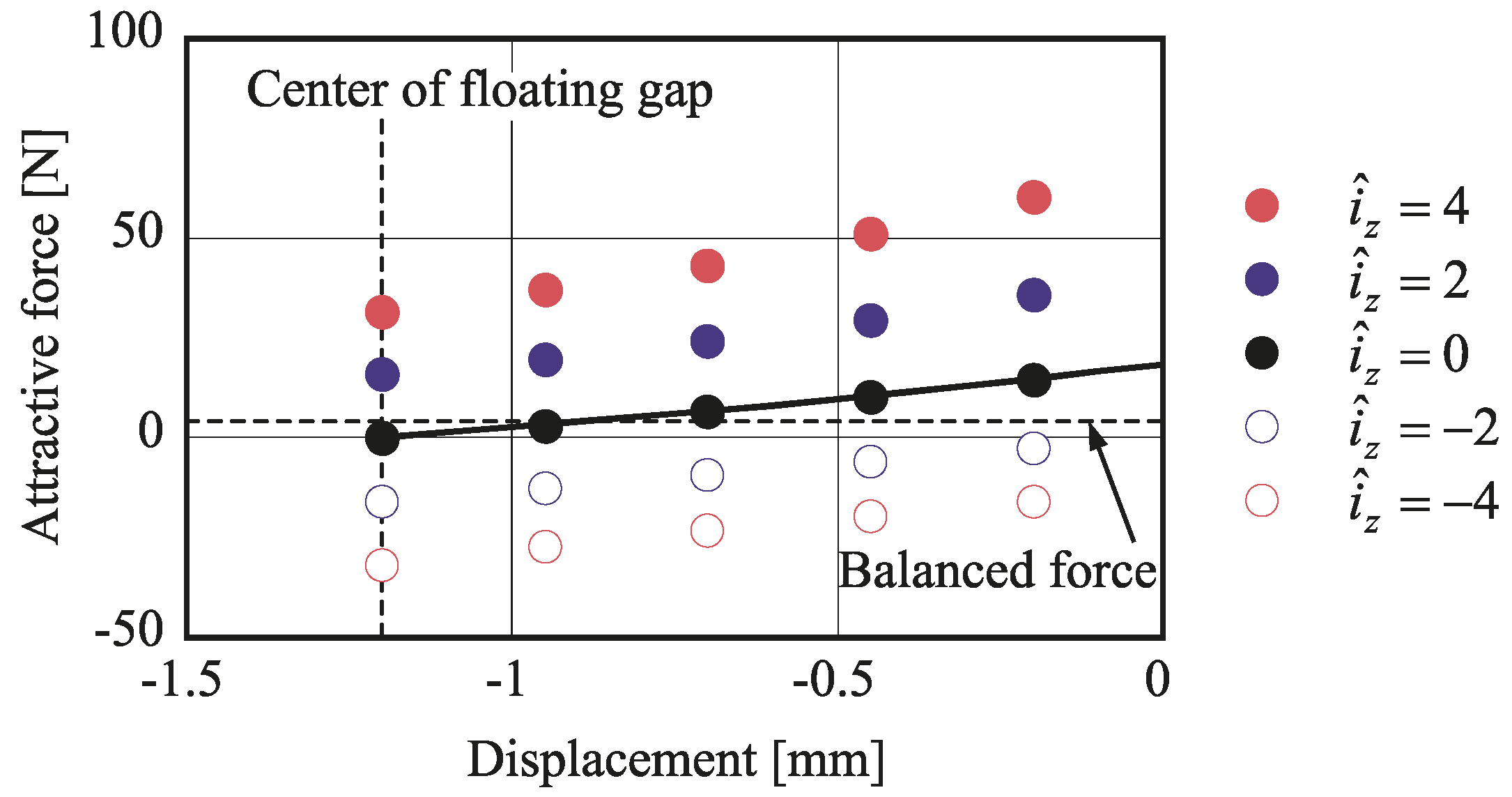
Figure 7 shows an analysis model of the magnetic suspension system. It shows an example of the contour diagram of the magnetic flux density when = 0, 1 A. The floator is at the center of the gap between the upper and lower electromagnet units. The magnetic fluxes of the upper and lower electromagnet units are same when the coil current is zero. When the coil current is increased, the magnetic flux from the upper electromagnet unit to the floator increases, and the flux from the lower unit to the floator decreases. Therefore, the upward force is increased by the coil current. Figure 8 shows a relation between the attractive force and the displacement of the translational motion along the z axis for various value of . The displacement 0 in the horizontal axis represents the position where the floator contacts the upper limiter, and the positive value in the vertical axis represents upward force. The equilibrium displacement is −0.9 mm when = 0 A, and the equivalent negative stiffness along the z axis is expected to be 13,000 N/m. Moreover, at the around the equilibrium displacement is expected to be 8 N/A.
4. Parameter Identification
First, the parameters related to the translational motion are identified. The mass of the floator is measured with a weight. The equivalent electromagnet coefficients are estimated from the frequency characteristics of the PD-controlled system experimentally. The transfer function of the PD-controlled system is given by
where
- : mass of the floator (kg),
- : feedback gain of velocity (derivative gain) (As/m),
- : feedback gain of displacement (proportional gain) (A/m).
The transfer function of the standard second-order system is given by
where
- : resonance angular frequency,
- : damping coefficient.
Comparing Equation (7) with Equation (8), we get
The feedback gain of displacement is varied in several ways while the feedback gain of velocity is kept to be as small as possible without losing stability. Then the resonant angular frequency is measured for each value of the proportional gain. Figure 9a shows the relation between the square of the resonance angular frequency and the proportional feedback gain. The black dots represent experimental values. The line represents an approximate straight line for the experimental values. The red dot represents the intercept value which is obtained by extrapolating the approximate line. The parameter is obtained by multiplying the value at the intercept by the mass. The parameter is obtained from the slope of the approximate line.
Next, the parameters related to the rotation motions are identified in a similar way. The moment of inertia () is calculated from the geometric shape on the assumption that the floator is uniform in density. Figure 9b,c shows the relations between the square of the resonance angular frequency and the proportional feedback gain in the rotation motions. The coefficient values obtained from these experiments are listed in Table 1.
5. Design of Controller
Various control laws such are PD, PID and zero power control can be applied selectively to each mode. The feedback gains in each case are determined based on the pole assignment. Here, the procedures of determining the gains are described when the zero power control is applied to the translational motion.
Figure 10 shows the block diagram of the zero power controller. This controller corresponds to the “feedback controller” in Figure 6. The transfer function of the zero power control magnetic suspension system is given by
where
- : velocity feedback gain (As/m),
- : displacement feedback gain (A/m),
- : local current integral feedback gain (As).
The characteristic polynomial of the system with the desired poles is assumed to be given by
The coefficient is a parameter related to the response speed or the bandwidth of the system; the response speed gets faster as becomes larger. Meanwhile, the feedback gains also become larger. Theoretically, we can set to be arbitrarily large. Practically, however, the whole system falls into instability when the feedback gains are too large. Therefore, we determined the value of to be as large as possible without inducing unstable behavior. The coefficients and are parameters related to the damping characteristics. Because the Butterworth filter has desirable damping characteristics, we set these coefficients to be two, that is, = 2 and = 2 in the following experiment. The feedback gains are determined by comparing the coefficients of the denominator in the right-hand side of Equation (10) with the right-hand side of Equation (11). The controllers for the tilt motions are designed similarly.
6. Experiments
6.1. Frequency Characteristics
The frequency responses of the displacement to the equivalent disturbance are measured. Figure 11 shows the comparison of experimental and theoretical values in the translational motion along the z axis and the rotational motion around the x axis. The characteristics of the rotational motion around the y axis is similar to the latter. The solid lines represent the experimental values and the dashed lines represent the theoretical values. In measuring the frequency characteristics, the zero power is applied to the target mode and PID control is applied to the other modes.
The poles of the translational motion along the z axis is assigned with an angular frequency of , and rad/s. The poles of the tilt motions are assigned with an angular frequency of or and rad/s. The poles of the PID controls system are assigned with an angular frequency of (rad/s). The experimental and theoretical values in gain are accordant up to 20 Hz in (a) and 10 Hz in (b). However, some discrepancy is observed between them at high frequency. This may be caused by the eddy current in the solid poles and the floator.
6.2. Inter-Axis Interferences
When the zero power control was applied to the three modes, the current of each coil and the equivalent currents converged to zero. Then, interferences among the modes are examined experimentally by adding equivalent rectangular-wave disturbances. The equivalent disturbance of the translational motion along z axis is added to the mode control current in Figure 6. The disturbance to the tilt motions are applied similarly. The parameters of the characteristic polynomial in Equation (11) were selected as
- rad/s,
- , .
Also, the controllers of the tilt motions are designed by the same way. The parameters are selected as
- rad/s,
- , ,
- rad/s,
- , .
The amplitude and frequency of the added disturbances are
- 1.27 N0-p, 0.5 Hz for along the z axis,
- 3.76 × 10⁻³ Nm0-p, 0.75 Hz for around the x axis,
- 3.76 × 10⁻³ Nm0-p, 1.0 Hz for around the y axis.
Figure 12 shows the output equivalent current of each controller. The shown current is calculated by subtracting the applied disturbance signal from the actual current. The current of each coil converged to zero due to the zero power control.
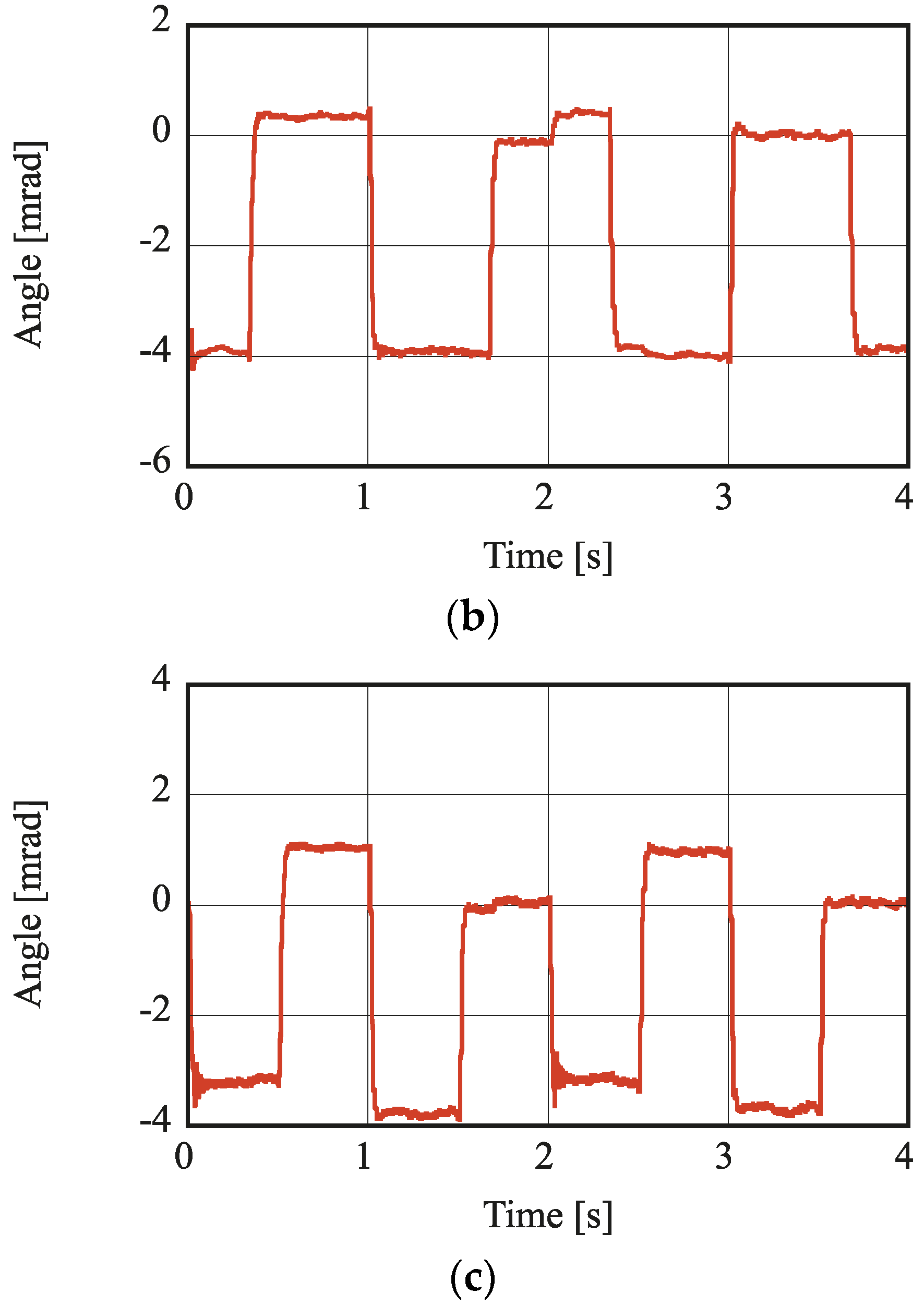
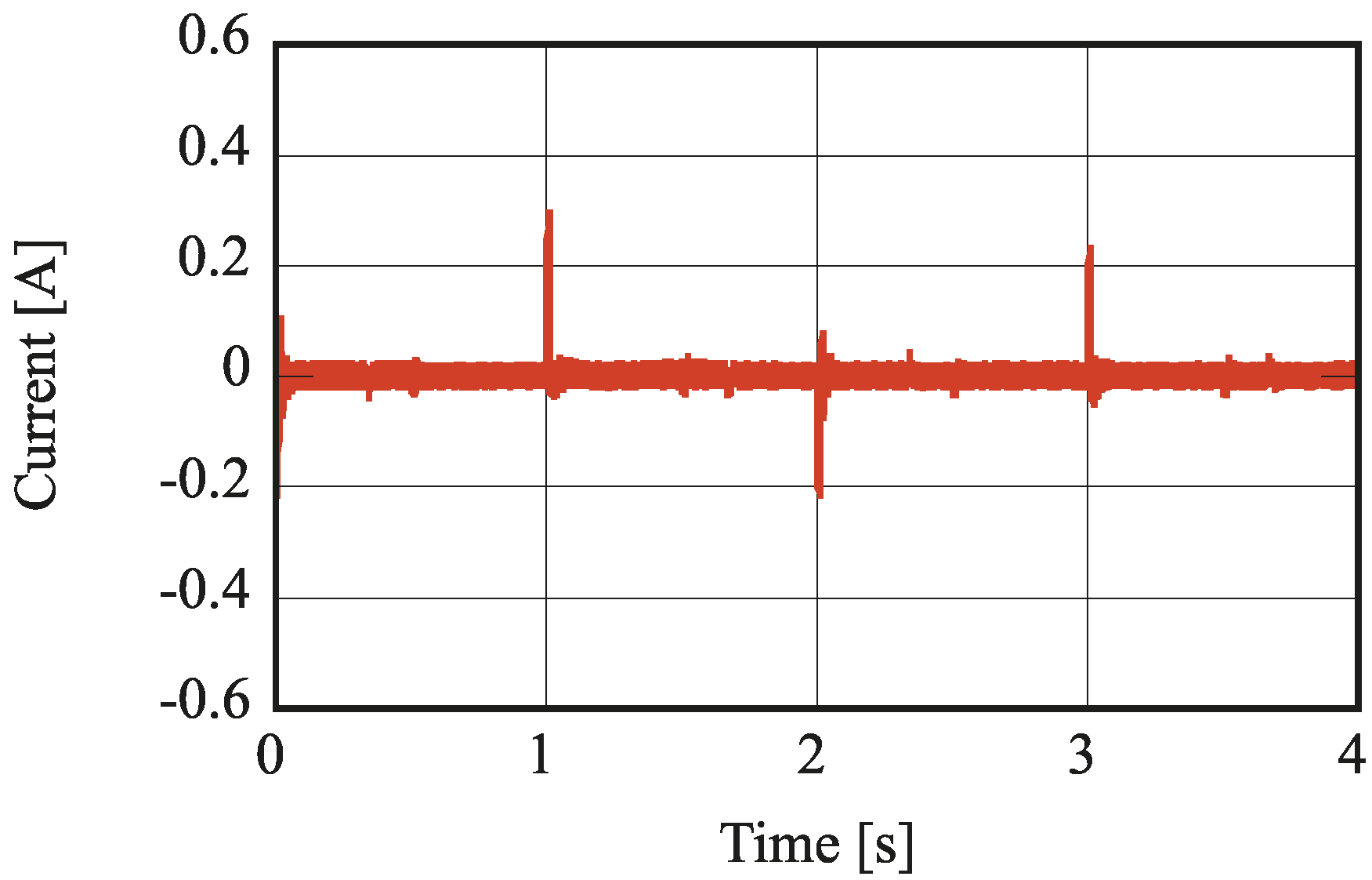
Figure 13 shows the displacement and the angle to the disturbance. The vertical axis in Figure 13a represent the displacement of the floator contacted with the limiter of the upper electromagnet of 0 mm. The displacement of the translational motion along the z axis is 0.53 mm when the zero power control is applied without a disturbance. This value is different from the analyzed value of 0.9 mm. The difference is due to the difference in magnetic flux density between the upper and lower permanent magnets. In Figure 13b,c, the offset angle of the tilt motions are caused by an unbalance of the floator when the zero power control is applied. The displacement of the translational motion along the z axis is less affected by the disturbance torque on tilt motions. The anglea of the tilt motions are affected more by the disturbance force for the translational motion along the z axis. The interference between the two rotational motions is small. As an example, the coil current of the electromagnet 1 is shown in Figure 14. The equivalent currents of three degrees-of-freedom converge to zero. Also, the current of each magnetic coil converges to zero.
7. Rotation
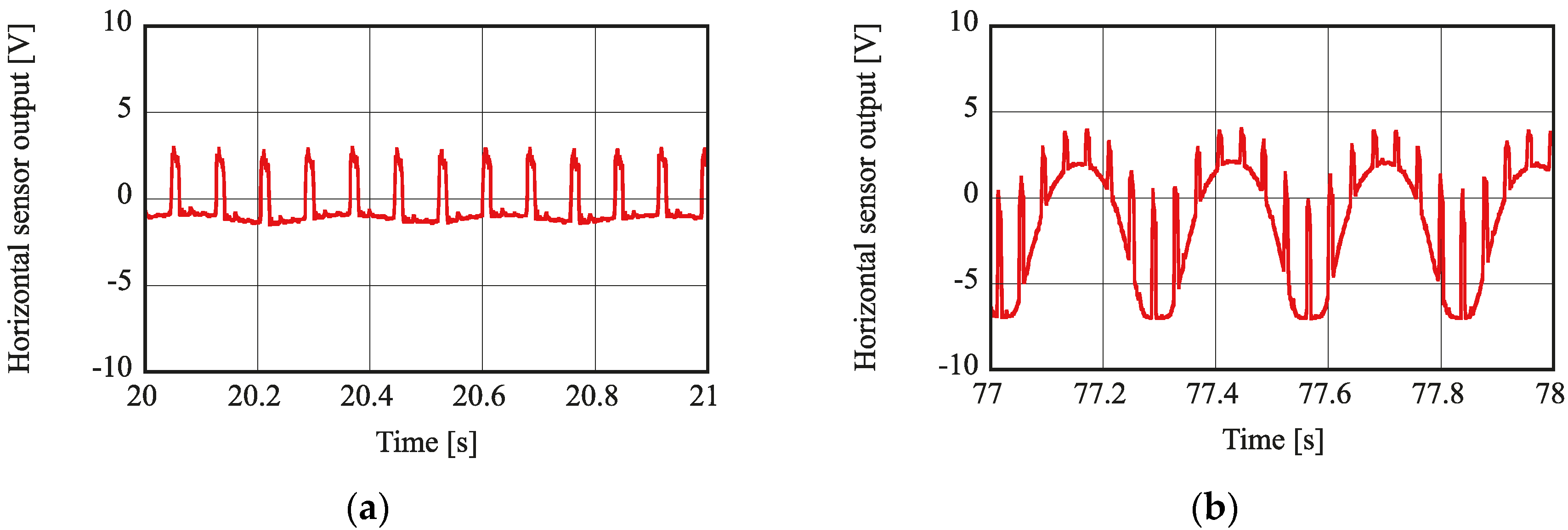
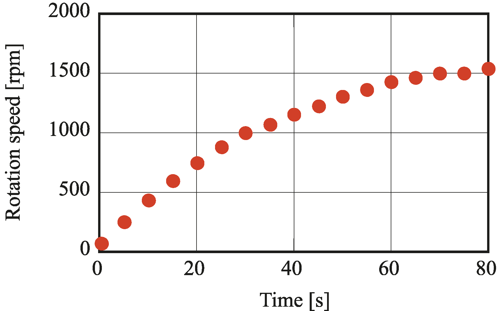
The floator is rotated around the z axis using the principle of induction motor. Four-phase AC signals are added to the control signal (current) of the coils. The rotational speed is measured by the horizontal displacement sensor. The frequency and amplitude of the input signal are 200 Hz and 0.4 A0-p. In this experiment, the zero power control is applied to the three modes. Figure 15 shows a relation between time and the rotation speed. The floator starts to rotate at 0 s. A black marker is pasted on the side of the floator. A reflective photo interrupter is used for the displacement sensor for measuring the horizontal direction. The output voltage of the photo interrupter generates pulse signal when the reflecting signal is blocked during passing the black marker. The rotation speed is measured from the pulses. Also, the output of the photo interrupter fluctuates due to the motion of the horizontal displacement. Figure 16 shows the output of the displacement sensor for the horizontal direction around 20 s and around 77 s after the rotation starts. The resolution of this measurement is 1 ms. The output signal is fluctuating like a sinusoidal wave due to the unbalance of the floator. The fluctuation of the floator increases as the rotation speed of the floator approached to the critical speed at 77 s. When the rotation speed approaches a critical speed, the floator collides with the horizontal displacement sensor unit. Therefore, the rotational signal is stopped manually at 78 s. The bias magnetic flux generated by the permanent magnet does not fluctuate according to the rotation around the z axis in the fabricated magnetic pole structure. Therefore, the floator can rotate under the zero power control without any special control.
8. Conclusions
A compact axial magnetic bearing with a function of two-tilt-motion control was proposed. It is characterized by new magnetic pole configurations: four poles with coil surrounding one common pole at the center in the stator and a permanent magnet at the surface opposite to the common pole in the rotor. The permanent magnet generates a bias flux. The bias magnetic flux does not fluctuate according to the rotation around the z axis in the proposed magnetic pole structure. Therefore, the proposed magnetic pole structure is suitable for the axial magnetic bearing with zero power control. An experimental apparatus without shaft to the axial disk of the rotor was designed and fabricated for studying the characteristics independently. Because the number of control currents (four) is larger than the number of freedom of motion to be controlled (three), mode control was applied in designing the control system. Three control laws such as PD, PID and zero power control were selectively applied to each mode. When the zero power control was applied to the three modes, the equivalent control current of each mode and resultantly the current of each coil converged to zero. In addition, the interferences among the modes were studied experimentally. The rotation of the floator was achieved by adding four-phase AC signals to the control currents of the coils.
Author Contributions
Ishino, Y. and Mizuno, T. wrote the paper. Ishino, Y. performed the experiments; Yamaguchi, D. contributed the design of the mechanisms; Hara, M. contributed the analyses of the data; Takasaki, M. contributed the design of the controller and electric circuit.
Conflicts of Interest
The authors declare no conflict of interest. The founding sponsors had no role in the design of the study; in the collection, analyses, or interpretation of data; in the writing of the manuscript, and in the decision to publish the results.
References
- Jayawant, B.V. Electromagnetic Levitation and Suspension Technique; Edward Arnold Publishers Limited: London, UK, 1981; pp. 1–17. [Google Scholar]
- Ohtsuka, T.; Kyotani, Y. Superconducting Levitated High Speed Ground Transportation Project in Japan. IEEE Trans. Magn. 1975, 11, 608–614. [Google Scholar] [CrossRef]
- Schweitzer, G.; Bleuler, H.; Traxler, A. Active Magnetic Bearings: Basics, Properties and Applications of Active Magnetic Bearings; Hochschulverlag AG an der ETH: Zurich, Switzerland, 1994; pp. 1–239. [Google Scholar]
- Brunet, M. Analysis of the Performance of an AMB Spindle in Creep Feed Grinding. In Proceedings of the 4th International Symposium on Magnetic Bearing, Zurich, Switzerland, 23–26 August 1994; pp. 519–524. [Google Scholar]
- Higuchi, T.; Horikoshi, A.; Komori, T. Development of an Actuator for Super Clean Rooms and Ultra High Vacuum. In Proceedings of the 2nd International Symposium on Magnetic Bearings, Tokyo, Japan, 12–14 July 1990; pp. 115–122. [Google Scholar]
- Matsuda, K.; Kita, T.; Okada, Y.; Masuzawa, T.; Ohishi, T.; Taenaka, Y.; Yamane, T. Radial-Type Self-Bearing Motor for Nonpulsatile-Type Artificial Heart. JSME Int. J. Ser. C Mech. Syst. Mach. Elem. Manuf. 2000, 43, 941–948. [Google Scholar] [CrossRef]
- Henrikson, C.; Lyman, J.; Studer, P. Magnetically Suspended Momentum Wheels for Spacecraft Stabilization. In Proceedings of the 12th Aerospace Sciences Meeting, Washington, DC, USA, 30 January–1 February 1974. [Google Scholar]
- Sabnis, A.V.; Dendy, J.B.; Schmitt, F.M. A Magnetically Suspended Large Momentum Wheel. J. Spacecr. Rocket. 1975, 12, 420–427. [Google Scholar] [CrossRef]
- Maruyama, Y.; Mizuno, T.; Takasaki, M.; Ishino, Y.; Kameno, H.; Kubo, A. Study on Control System for Active Magnetic Bearing Considering Motions of Stator. J. Syst. Des. Dyn. 2009, 3, 954–965. [Google Scholar] [CrossRef]
- Morishita, M.; Azukizawa, T. Zero Power Control Method for Electromagnetic Levitation System. Electr. Eng. Jpn. 1988, 108, 447–454. [Google Scholar] [CrossRef]
- Mizuno, T.; Takemori, Y. A Transfer-Function Approach to the Analysis and Design of Zero-Power Controllers for Magnetic Suspension System. Electr. Eng. Jpn. 2002, 141, 67–75. [Google Scholar] [CrossRef]
- Morishita, M.; Azukizawa, T.; Kanda, S.; Tamura, N.; Yokoyama, T. A New Maglev System for Magnetically Levitated Carrier System. IEEE Trans. Veh. Technol. 1989, 38, 230–236. [Google Scholar] [CrossRef]
- Morishita, M.; Akashi, M. Electromagnetic Non-Contact Guide System for Elevator Cars. In Proceedings of the Third International Symposium on Linear Drives for Industry Applications (LDIA 2001), Nagano, Japan, 17–19 October 2001; pp. 416–419. [Google Scholar]
- Yakushi, K.; Koseki, T.; Sone, S. 3 Degree-of-Freedom Zero Power Magnetic Levitation Control by a 4-Pole Type Electromagnet. In Proceedings of the International Power Electronics Conference IPEC-Tokyo 2000, Tokyo, Japan, 3–7 April 2000; pp. 2136–2141. [Google Scholar]
Figure 1.
Schematic view of the proposed axial magnetic bearing.
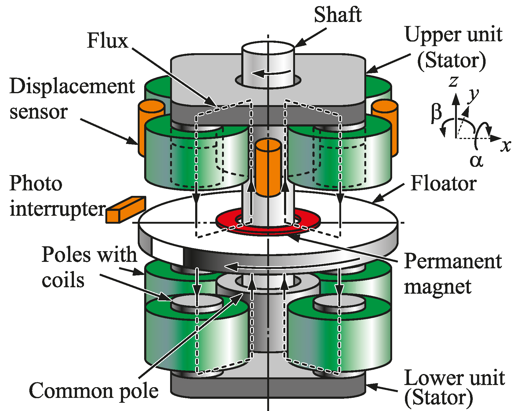
Figure 2.
Photograph of the fabricated three-degree-of-freedom magnetic suspension system.
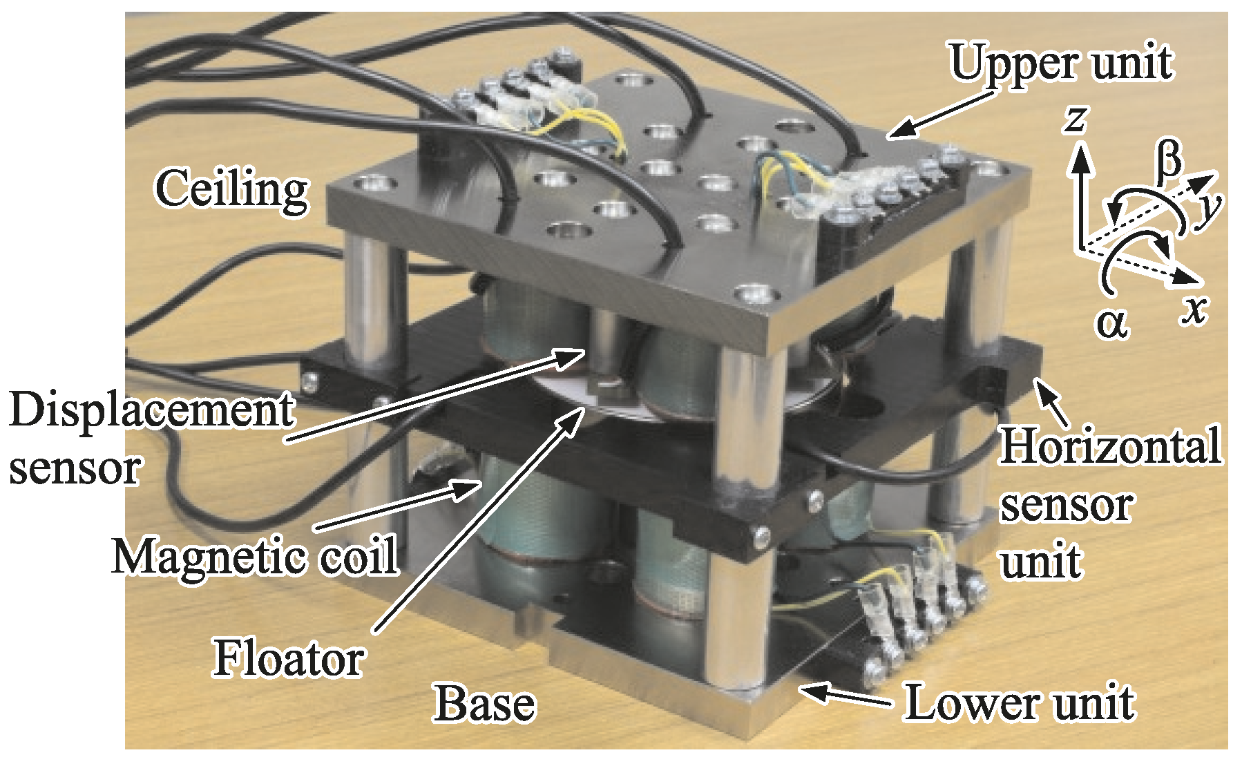
Figure 3.
Photograph of the upper electromagnet unit with displacement sensors.
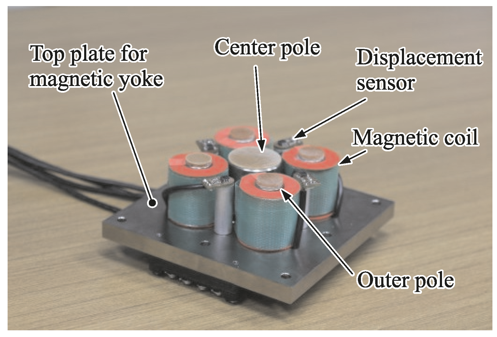
Figure 4.
Photograph of the floator attached permanent magnets and a sensor target.
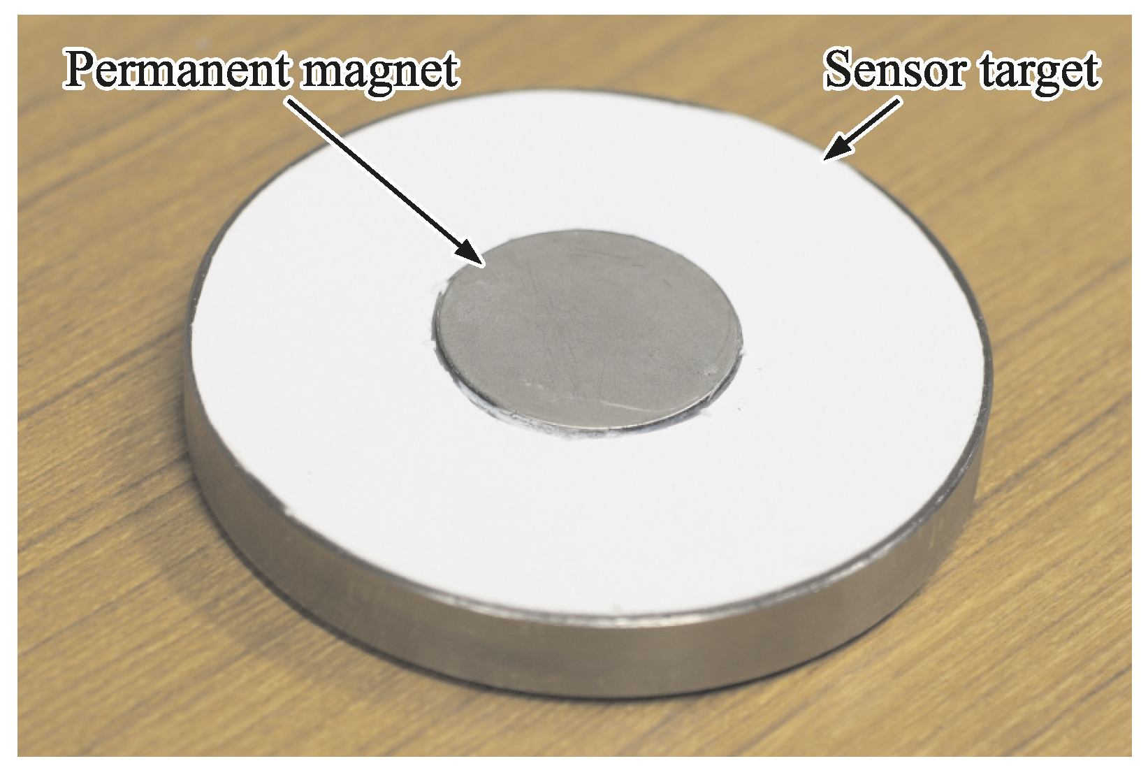
Figure 5.
Coordinate definition and the location of coils and sensors.
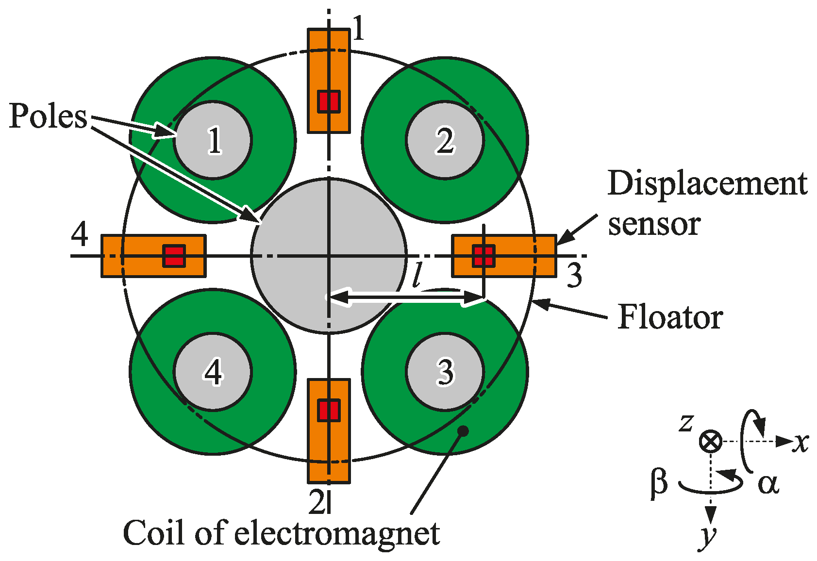
Figure 6.
Block diagram of the control system for the translational motion.
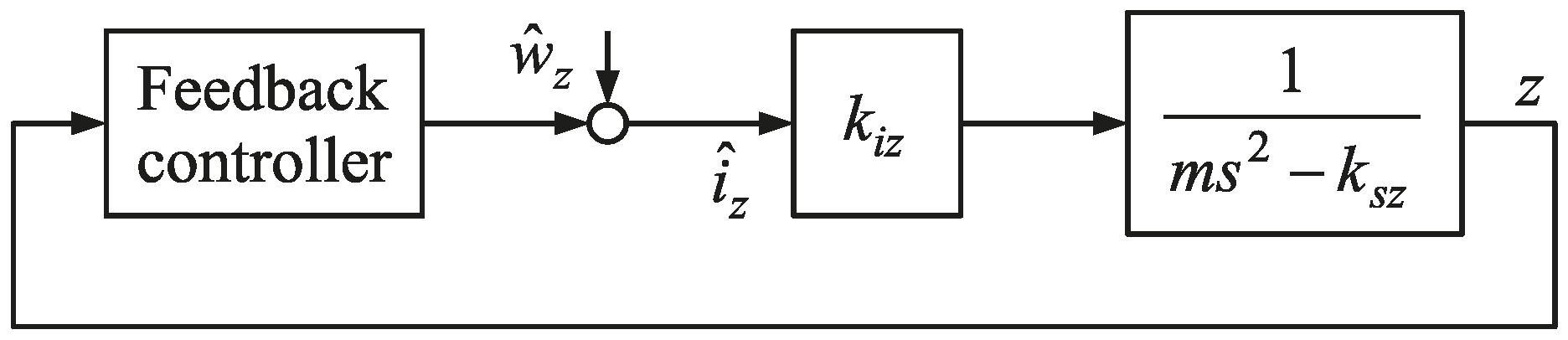
Figure 7.
Magnetic flux density in an analysis model with the proposed pole arrangement.
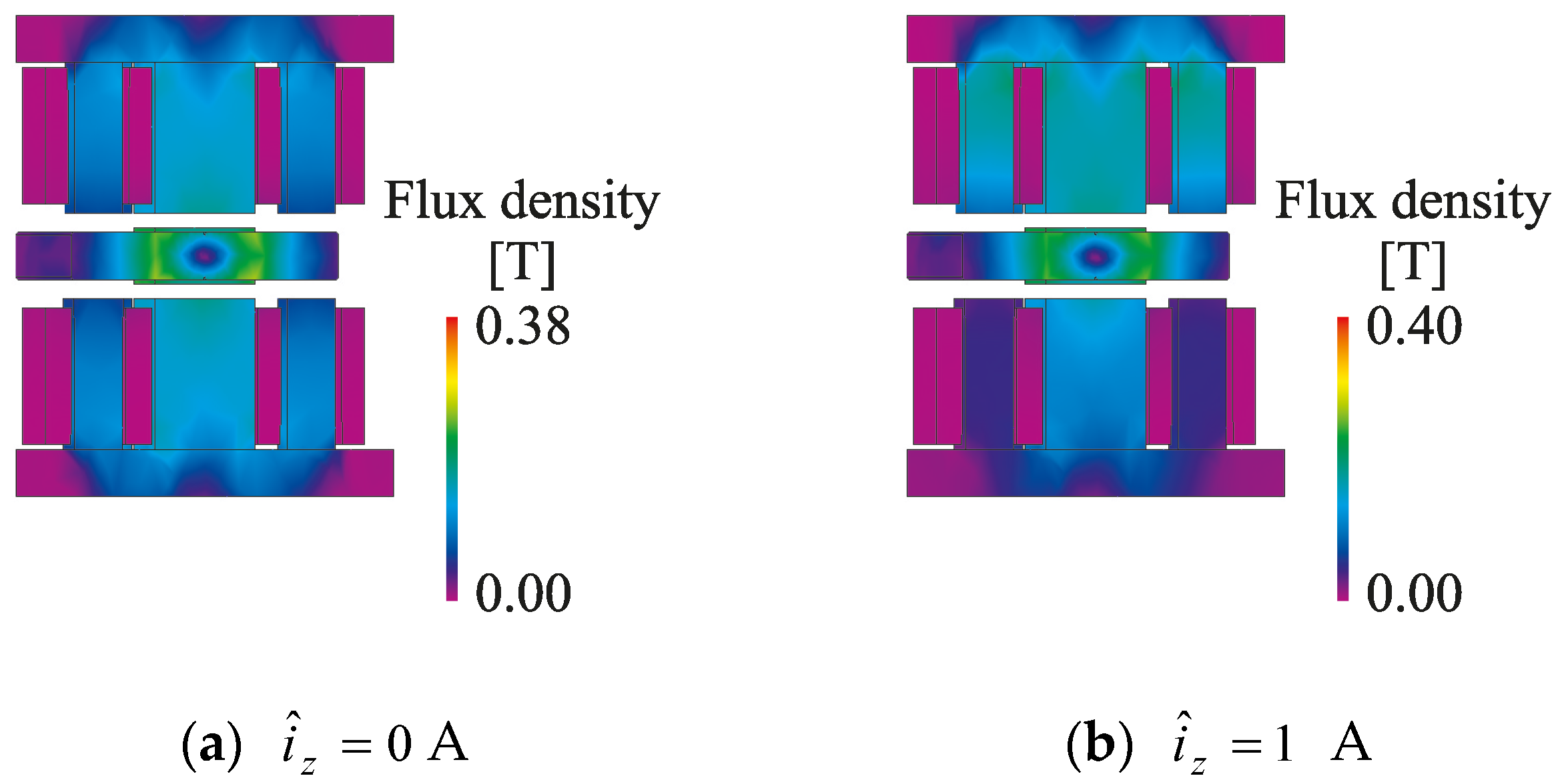
Figure 8.
Relation between the displacement of the floator and the attractive force when the equivalent current is applied (analytical results).
Figure 8.
Relation between the displacement of the floator and the attractive force when the equivalent current is applied (analytical results).

Figure 9.
Relation between the square of resonance angular frequency to the proportional gain (a) in the translational motion along the z axis; (b) in the rotational motion around the x axis; (c) in the rotational motion around the y axis.
Figure 9.
Relation between the square of resonance angular frequency to the proportional gain (a) in the translational motion along the z axis; (b) in the rotational motion around the x axis; (c) in the rotational motion around the y axis.
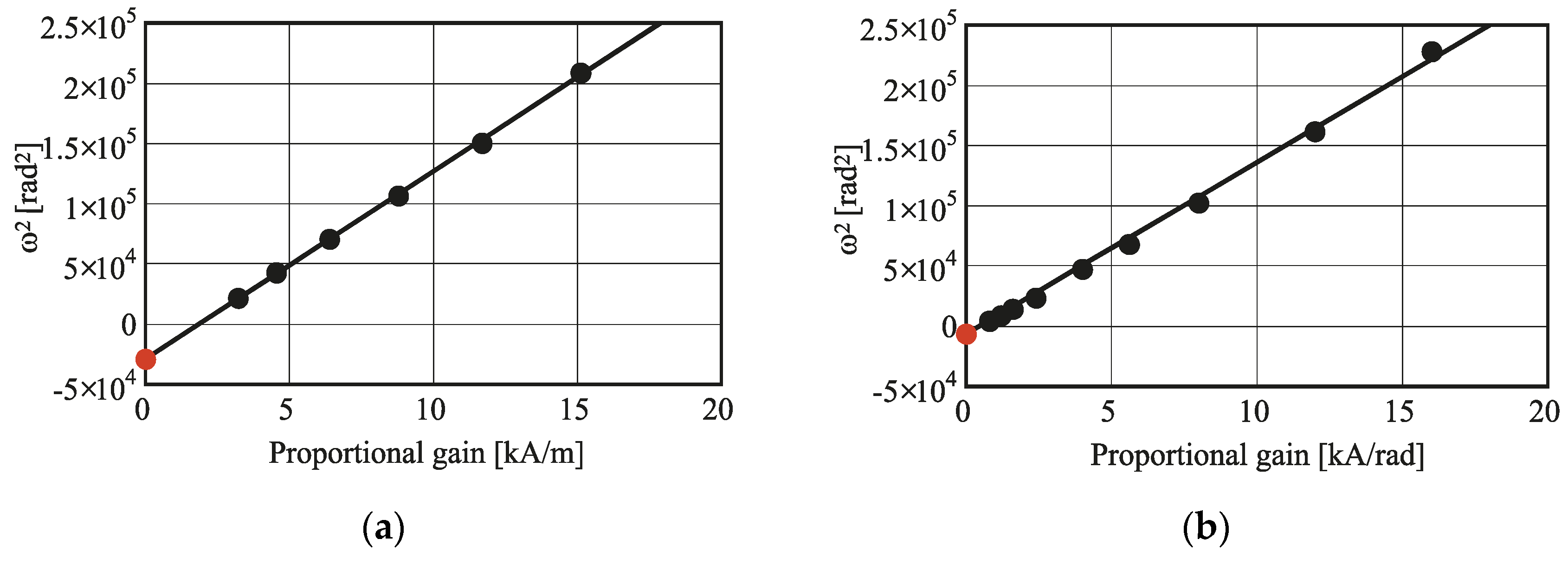
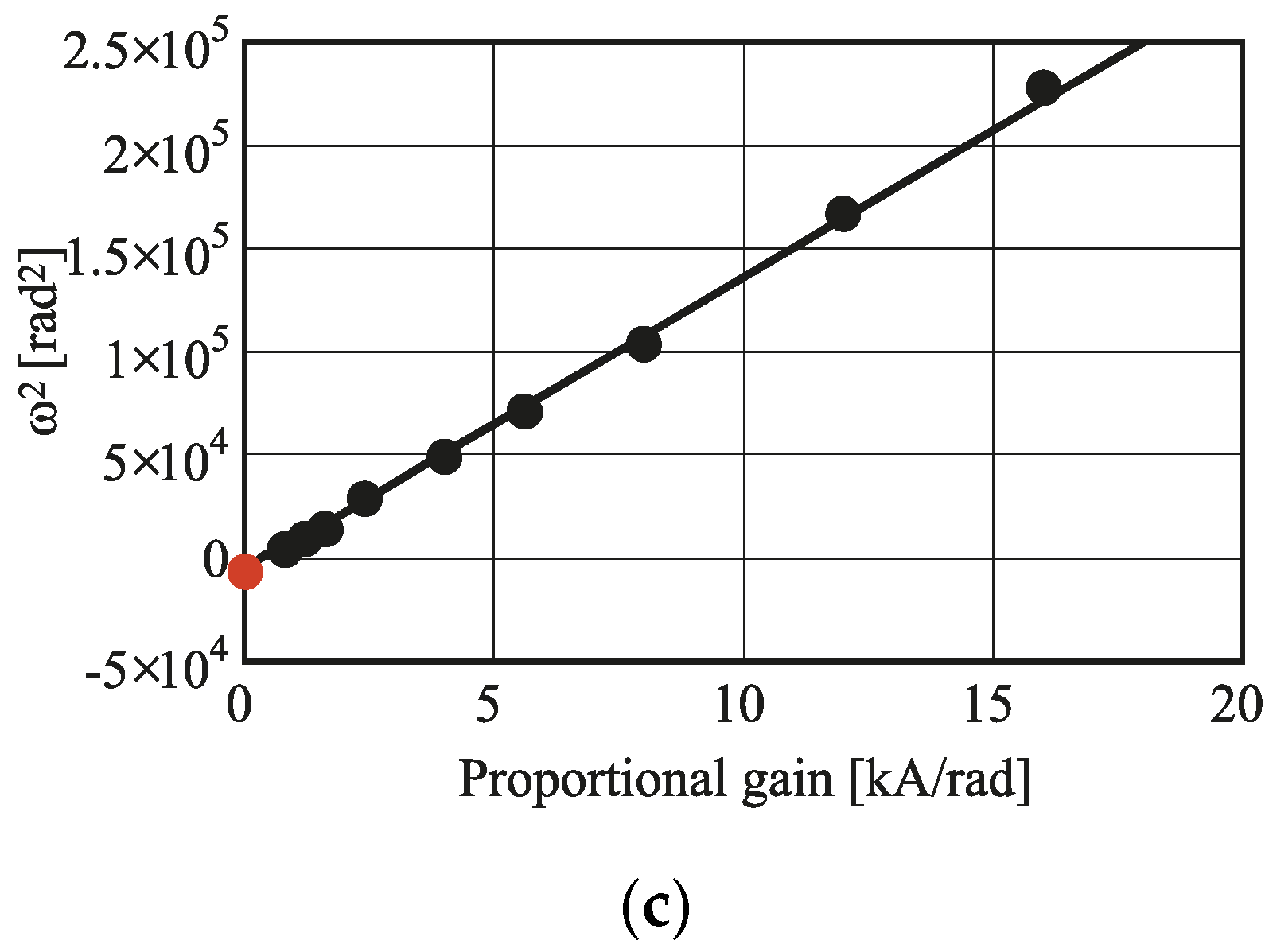
Figure 10.
Block diagram of zero power feedback controller for the translational motion along the z axis.
Figure 10.
Block diagram of zero power feedback controller for the translational motion along the z axis.
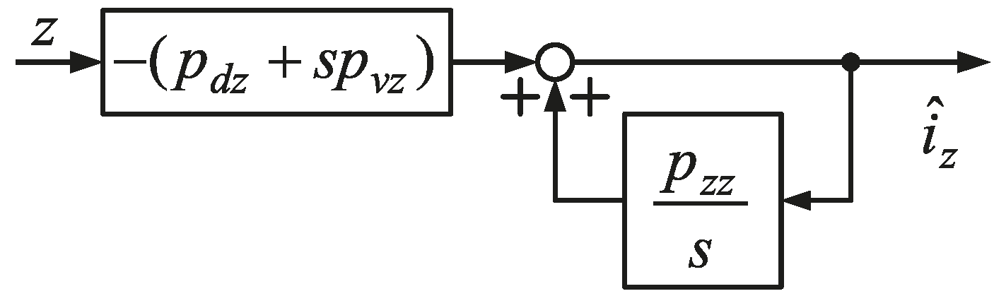
Figure 11.
Frequency characteristics of the simulated disturbance to the displacement with the zero power control. (a) Translational motion along the z axis; (b) Rotational motion around the x axis.
Figure 11.
Frequency characteristics of the simulated disturbance to the displacement with the zero power control. (a) Translational motion along the z axis; (b) Rotational motion around the x axis.
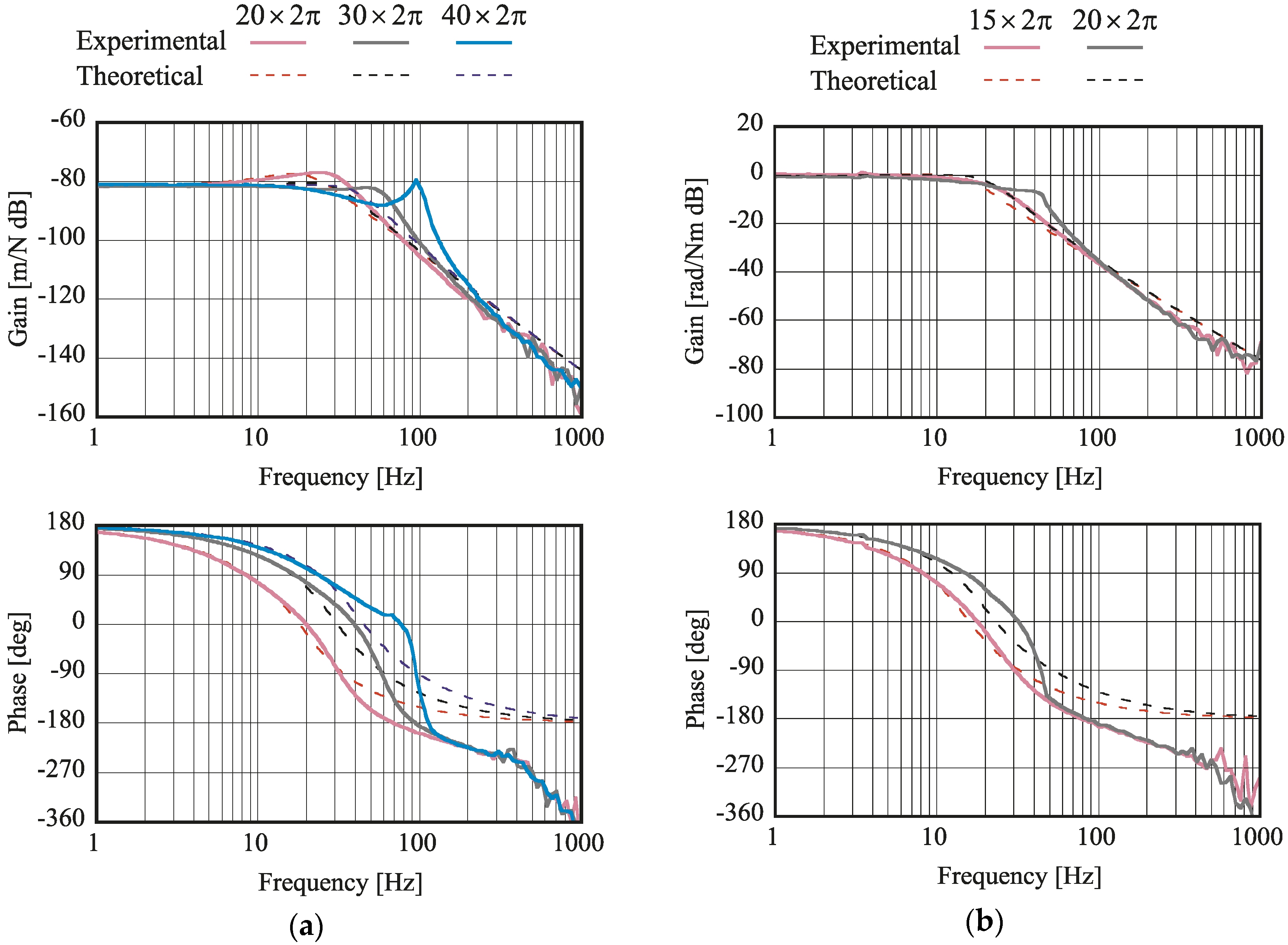
Figure 12.
Step characteristics of equivalent current. (a) Translational motion along the z axis; (b) Rotational motion around the x axis; (c) Rotational motion around the y axis.
Figure 12.
Step characteristics of equivalent current. (a) Translational motion along the z axis; (b) Rotational motion around the x axis; (c) Rotational motion around the y axis.
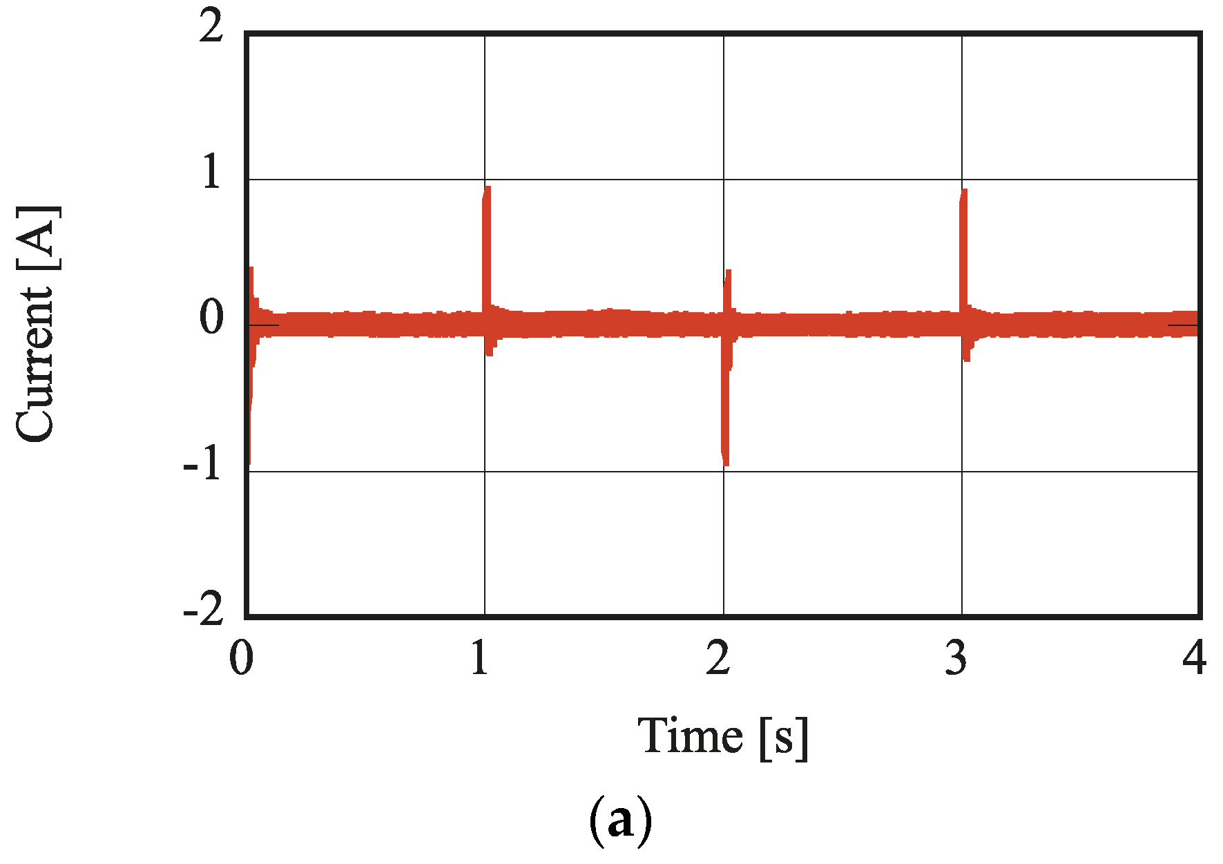
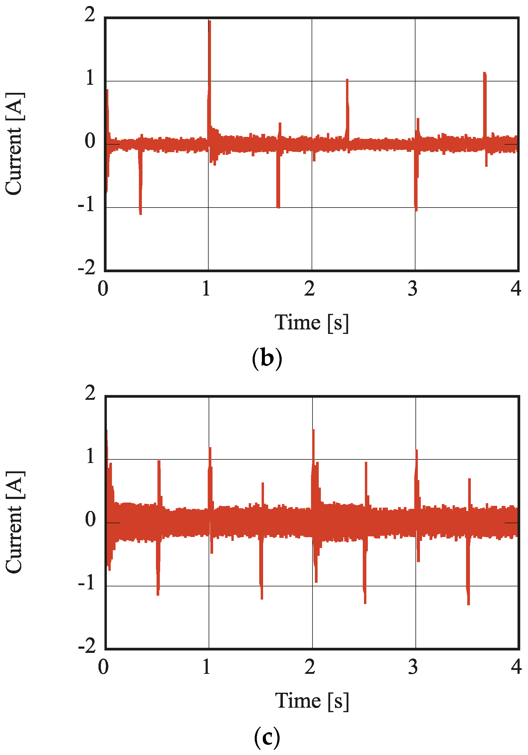
Figure 13.
Step characteristics of the displacement and angles. (a) Displacement along the z axis; (b) Angle around the x axis; (c) Angle around the y axis.
Figure 13.
Step characteristics of the displacement and angles. (a) Displacement along the z axis; (b) Angle around the x axis; (c) Angle around the y axis.
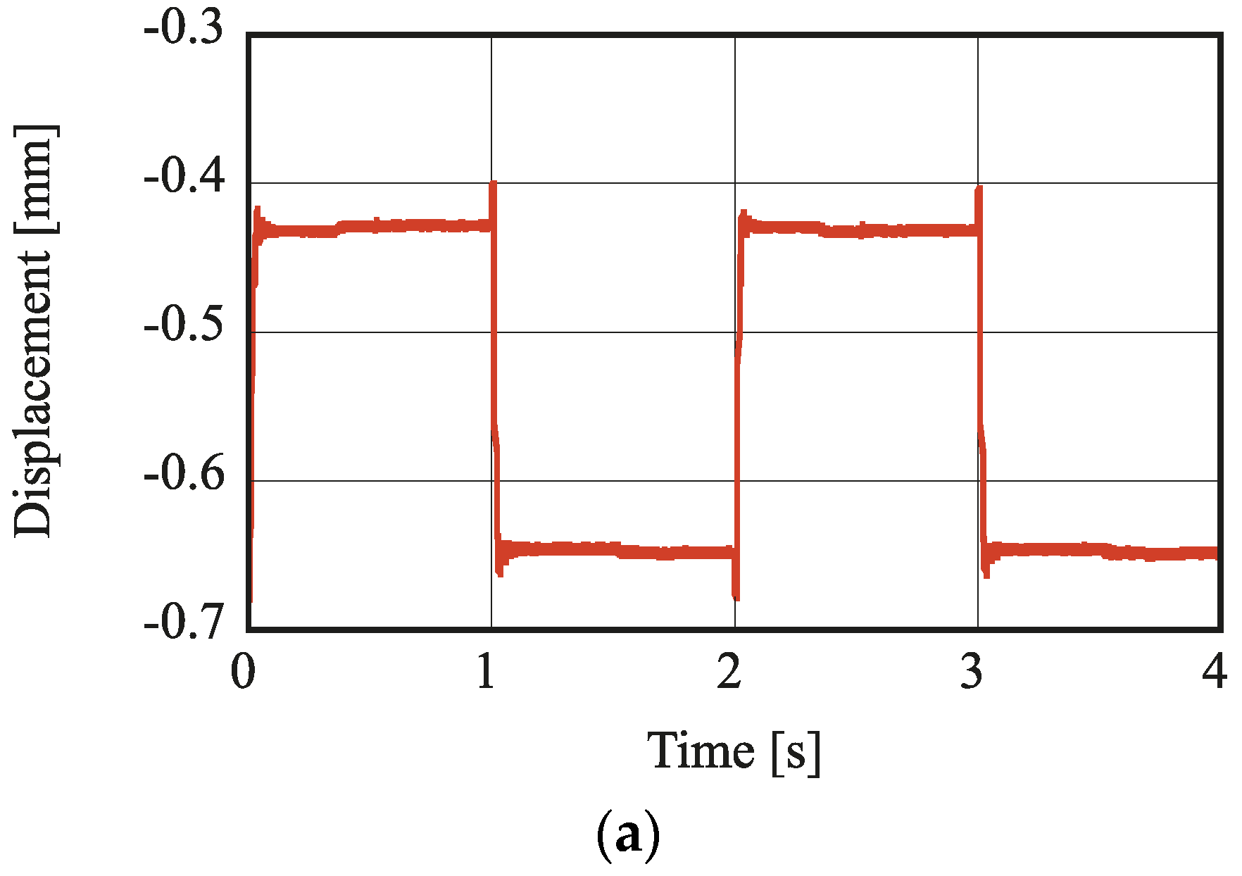

Figure 14.
Step characteristics of the coil current in the electromagnet 1.

Figure 15.
Time history of rotation speed.

Figure 16.
Output of horizontal sensor. One pulse per rotation is generated which is used to estimate the rotational speed. (a) 20 seconds after the start of rotation; (b) approaching to the critical speeds.
Figure 16.
Output of horizontal sensor. One pulse per rotation is generated which is used to estimate the rotational speed. (a) 20 seconds after the start of rotation; (b) approaching to the critical speeds.

Table 1.
Identified parameters.
| Parameters | m | ksz | kiz |
| Along z axis | 0.408 kg | 11,600 N/m | 6.35 N/A |
| Parameters | I | ksα, ksβ | kiα, kiβ |
| Around x axis | kgm2 | 1.00 Nm/rad | Nm/A |
| Around y axis | kgm2 | 1.00 Nm/rad | Nm/A |
© 2017 by the authors. Licensee MDPI, Basel, Switzerland. This article is an open access article distributed under the terms and conditions of the Creative Commons Attribution (CC BY) license (http://creativecommons.org/licenses/by/4.0/).
Share and Cite
MDPI and ACS Style
Ishino, Y.; Mizuno, T.; Takasaki, M.; Hara, M.; Yamaguchi, D. Development of a Compact Axial Active Magnetic Bearing with a Function of Two-Tilt-Motion Control. Actuators 2017, 6, 14. https://doi.org/10.3390/act6020014
AMA Style
Ishino Y, Mizuno T, Takasaki M, Hara M, Yamaguchi D. Development of a Compact Axial Active Magnetic Bearing with a Function of Two-Tilt-Motion Control. Actuators. 2017; 6(2):14. https://doi.org/10.3390/act6020014
Chicago/Turabian StyleIshino, Yuji, Takeshi Mizuno, Masaya Takasaki, Masayuki Hara, and Daisuke Yamaguchi. 2017. "Development of a Compact Axial Active Magnetic Bearing with a Function of Two-Tilt-Motion Control" Actuators 6, no. 2: 14. https://doi.org/10.3390/act6020014
Note that from the first issue of 2016, this journal uses article numbers instead of page numbers. See further details here.