
Adaptive Numerical Modeling of Tsunami Wave Generation and Propagation with FreeFem++


1
Laboratoire de Mathématiques Raphaël Salem, Université de Rouen Normandie, CNRS UMR 6085, Avenue de l’Université, BP 12, F-76801 Saint-Étienne-du-Rouvray, France
2
Univ. Grenoble Alpes, Univ. Savoie Mont Blanc, CNRS, LAMA, 73000 Chambéry, France
*
Author to whom correspondence should be addressed.
†
These authors contributed equally to this work.
Geosciences 2020, 10(9), 351; https://doi.org/10.3390/geosciences10090351
Submission received: 31 July 2020
/
Revised: 29 August 2020
/
Accepted: 1 September 2020
/
Published: 4 September 2020
(This article belongs to the Special Issue Interdisciplinary Geosciences Perspectives of Tsunami Volume 3)
Abstract
:A simplified nonlinear dispersive Boussinesq system of the Benjamin–Bona–Mahony (BBM)-type, initially derived by Mitsotakis (2009), is employed here in order to model the generation and propagation of surface water waves over variable bottom. The simplification consists in prolongating the so-called Boussinesq approximation to bathymetry terms, as well. Using the finite element method and the FreeFem++ software, we solve this system numerically for three different complexities for the bathymetry function: a flat bottom case, a variable bottom in space, and a variable bottom both in space and in time. The last case is illustrated with the Java 2006 tsunami event. This article is designed to be a pedagogical paper presenting to tsunami wave community a new technology and a novel adaptivity technique, along with all source codes necessary to implement it.
Keywords:
tsunami wave; finite elements; mesh adaptation; domain adaptation; co-seismic displacements; tsunami wave energy; FreeFem++; unstructured meshesPACS:
47.35.Bb; 02.60.-xMSC:
76B15; 65N30; 65N50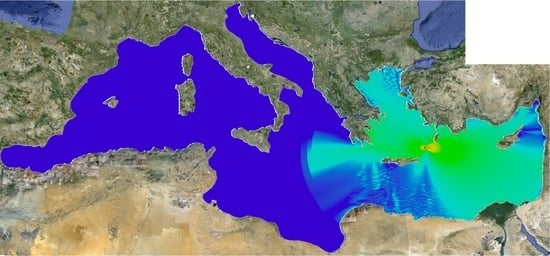
1. Introduction
Tsunami waves represent undeniably a complex natural process. Moreover, they represent a major risk for exposed coastal areas, including the local populations, infrastructure, etc. The present work (the present paper is also available as a preprint [1]) is devoted to the modeling tsunami generation and propagation processes. Moreover, this article is designed as a tutorial paper in order to show to the readers how easily these processes can be modeled in the framework of the FreeFem++, which is a free software (under the LGPL license). FreeFem++ offers a large variety of triangular finite elements (linear and quadratic Lagrangian elements, discontinuous , Raviart–Thomas elements, etc.) to solve Partial Differential Equations (PDEs). It is an integrated product with its own high level programming language and a syntax close to mathematical formulations, making the implementation of numerical algorithms very easy. Among the features making FreeFem++ an easy-to-use and highly adaptive software, we recall the advanced automatic mesh generator, mesh adaptation, problem description by its variational formulation, automatic interpolation of data, color display on line, postscript printouts, etc. The FreeFem++ programming framework offers the advantage of hiding all technical issues related to the implementation of the finite element method [2].
Traditionally, tsunami waves are modeled using hydrostatic models [3,4,5,6]. In the present manuscript, we employ a non-hydrostatic Boussinesq-type system to be specified below. This class of models is distinguished by the application of the so-called Boussinesq approximation [7]. They can be used to study a variety of water wave phenomena in harbors, coastal dynamics, and, of course, tsunami generation and propagation problems [8,9,10,11,12].
In this study, we consider an simplified Benjamin–Bona–Mahony (sBBM) system derived by D. Mitsotakis (2009) in 2D over a variable bottom in space and in time [13]:
where
Constants , , are real parameters and g is the acceleration due to gravity. System (1) is an asymptotic approximation to the three-dimensional full Euler equations describing the irrotational free surface flow of an ideal fluid [14,15], which is bounded below by and above by the free surface elevation (cf. Figure 1). The system (1) can be considered as a generalization of the classical Boussinesq system put forward by D. Peregrine [16,17].
The variables in (1) are and are proportional to position along the channel and time, respectively. being proportional to the deviation of the free surface departing from its rest position and being proportional to the horizontal velocity of the fluid at some height. In our study, we suppose that , with the characteristic wave amplitude a (in other words, is the difference between the water free surface and the still water level). In addition, we set be the wave length. Moreover, we limit ourselves to the case where (there are no dry zones in our computations).
This paper is organized as follows. In Section 2, we present the space and time discretization of a simplified version (4) of Equations (1). In Section 3, we present the new domain adaptation technique. In Section 4, we establish the convergence of our numerical code, which validates the adequacy of the chosen finite element discretization. Then, with this code, we simulate the propagation of a tsunami-like wave generated by the moving bottom (e.g., an earthquake). We present several test cases in various regions of the world. First, we take a Mediterranean sea-shaped computational domain with flat bottom, and we solve the sBBM system (Please, notice that BBM–BBM (1) and sBBM (4) systems coincide over flat bottoms.) (1) in it. The mesh in this study is generated from a space image. Then, we consider the Java island region with real world bathymetry. Finally, we apply this solver to simulate a realistic example of a tsunami wave near the Java island which took place in 2006. The main conclusions of this study are outlined in Section 5.
2. Discretization of the sBBM System
In this section, we present the spatial discretization of (1) using Finite Element Method (FEM) with continuous piecewise linear elements. For the time marching scheme, we use an explicit second order Runge–Kutta method.
2.1. Spatial Discretization
We let be a convex, plane domain, and be a regular, quasi-uniform triangulation of with triangles of maximum size . Setting be a finite-dimensional, where is the set of all polynomials of degree with real coefficients and denoting by the standard inner product on , we consider the weak formulation of System (1): find such that , we have:
For simplicity, we set , so that System (2) can be rewritten in the following way:
However, the model presented above contains some drawbacks. In particular, when the bathymetry function contains steep gradients, it causes instabilities in the numerical solution. We have to mention that this problem is well-known in the framework of Boussinesq-type equations [18]. In order to avoid this kind of problems and to have a robust numerical model, we take two measures. First of all, we perform the smoothing of the bathymetry data which is fed into the model. In this way, we avoid noise in the bathymetry gradient. As a second and more radical step, we neglect higher order derivatives of the bathymetry function as it was proposed earlier in Reference [13]. Thus, from now on we shall use the following system of equations:
with
and
Several intermediate computations are reported in Appendix A. We would like to underline the fact that the performed simplification allows us to gain in numerical model stability and robustness at the price of some higher order bathymetry effects.
2.2. Time Marching Scheme
Our method is based on the explicit second order Runge–Kutta scheme. For that, let us denote by and the approximate values at time and , respectively and by the time step size. Then, owing to (4), the unknown fields at time are defined as the solution of the following system:
where
and
3. New Domain Adaptation, Domains Computation and Initial Data
We present here the new domain adaptation technique that will be compared in the sequel with the mesh adaptation used in FreeFem++. In order to complete the literature review, we would like to mention that alternative approaches exist, see, e.g., Reference [19,20].
3.1. New Domain Adaptation Technique
Since some computation domains for many applications (here for tsunami waves [21]) may be huge and the initial data is concentrated in a small domain, a circle or a rectangle , before starting to propagate in the domain, we present here an idea to build a moving computation domain around the solution only, as when we use a mesh adaptation. The difference between these two methods is that the moving domain will be a cut from the initial one, i.e., all initial vertices, edges, and boundary labels are conserved, and a new label is defined for the new boundary; since the mesh adaptation technique does not conserve the initial vertices and edges, when we interpolate the solution from the old to new mesh, we will lose some information in the mesh adaptation technique but not with the moving domain.
Firstly, we cut from the initial mesh Thinit a circle or a rectangle zone Th where our initial solution lives (using trunc in FreeFem++, see (a) in Figure 2), we let uadapt be the initial solution used for the domain adaptation, and we follow this algorithm:
- We deduce the limit min max of Th on x and y direction (using boundingbox in FreeFem++).
- We increase the mesh from Th to Th1 by adding layers from the original mesh (using trunc in FreeFem++), the added zone is a size of epsadapt from each side, and we mapped uadapt to unew (using interpolate in FreeFem++, see (b) in Figure 2).
- We define a Heaviside function unewadapt which have a 1 value if the absolute value of unew is grater then or equal to a defined error (erradapt) by the user and 0 otherwise (see (c) in Figure 2).
- We smooth the function unewadapt (see (d) in Figure 2)) solving the following problem:with zero Dirichlet Boundary Condition (BC) only on the new boundary label of Th1 and a Neumann BC in the other boundary label. Here is the real coefficient that controls the smoothness of the solution and f=unewadapt.
- We define a Heaviside function ufinal which has a 1 value if the absolute value of usmadapt is greater then or equal to a defined error (erradapt) by the user and 0 otherwise (see (c) in Figure 2).
- We cut from Th1, the region where ufinal is grater then a defined isoline isoadapt by the user in order to obtain the final mesh Thnew (using trunc in FreeFem++), then we obtain the initial solution mapped over the final mesh using interpolate in FreeFem++, see (f) in Figure 2).
We use a reflective Boundary Condition (BC) on the new boundary, i.e., homogeneous Neumann BC for and homogeneous Dirichlet BC, for the velocity V. This choice is justified theoretically over flat bottom case in Reference [22]. Moreover, the homogeneous Neumann BC for can be shown to hold exactly in the full Euler equations on solid vertical walls; see Reference [23] (Section §2.1.4) for the proof.
3.2. Domains Computation
For the BBM–BBM system over a flat bottom, we use a mesh generated through a photo of the Mediterranean sea (a cut of the mesh around the Crete island is shown in Figure 3 at left panel), and, for the sBBM system over a variable bottom in space and in time, we use a mesh generated using an imported bathymetry for the sea near the Java island, which can be downloaded from the National Oceanic and Atmospheric Administration (NOAA) (https://maps.ngdc.noaa.gov/viewers/wcs-client/) website where, in this case, we remove the dry zone from our mesh and keep only the wet zone. We can smooth the bathymetric data obtained from NOAA (cf. Figure 4, left panel) by solving (8) with . For all simulations with realistic bathymetry, we use in (8) to smooth the initial bathymetry after the generation of the mesh (cf. Figure 4, right panel) in order to ensure the stability of the numerical method. We also mention that we change the depth close to the shoreline to 100 m in order to avoid the run-up problem in this study. Finally, all types of meshes used in our computations are depicted in Figure 5.
The bathymetry data downloaded from the NOAA website are in geographical degrees coordinates and we need to convert them back to meters and a Cartesian system. So, on the one hand, we must know the degree of Latitude (South and North) and of Longitude (West and East) of our domain where we can deduce the Latitude and the Longitude . On the other hand, we must take into account the spherical shape of the Earth, even if it does not play significant role because of the small spatial scale of the experiments. So, we know that the radius of the Earth near the equator is 6,378,137 km and near to the pole 6,356,752 km; thus, the radius of our domain equals to:
So, we move the mesh of our domain using the following translation ():
Finally, for the active generation case, since the fault plane is considered to be the rectangle with vertices located at (109.20508° (Lon), −10.37387° (Lat)), (106.50434° (Lon), −9.45925° (Lat)), (106.72382° (Lon), −8.82807° (Lat)) and (109.42455° (Lon), −9.74269° (Lat)), we will consider that our bottom displacement is concentrated on the big rectangle which is equidistant of 1° from each side of the initial fault plane, as in Figure 6 (left panel).
3.3. Initial Data
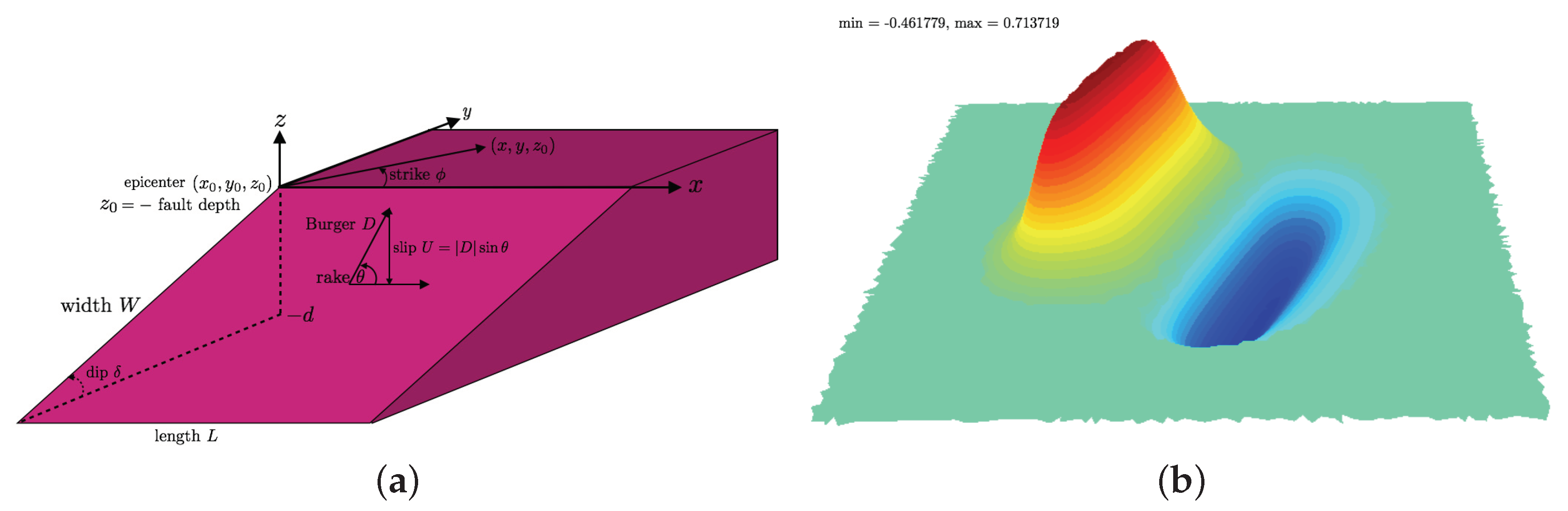
Tsunami waves considered in this study are generated by the co-seismic deformation of the Ocean’s or sea’s bottom due to an earthquake. The adopted modeling of the tsunami wave generation process is inspired by [10,13,24,25]. The co-seismic displacement is computed according to the celebrated Okada’s solution [26,27]. We assume the dip-slip dislocation process underlying the earthquake. The vertical component of displacement vector is given by the following formulas employing Chinnery’s notation, cf. [24,25]:
where
and
Here, W and L are the width and the length of the rectangular fault, are the points where we computes displacements, is the epicenter, , is the dip angle, is the rake angle, D is the Burgers’s vector, is the slip on the fault, is the strike angle which is measured conventionally in the counter-clockwise direction from the North (cf. Figure 7 (left)), are the Lamé constants derived from elastic-wave velocities: and , where is the crust density, is the compressional-wave (P–wave) velocity, is the shear-wave (S–wave) velocity. The Matlab script to compute the Okada solution can be downloaded at the following URL: https://mathworks.com/matlabcentral/fileexchange/39819-okada-solution/.
We shall distinguish here the two types of tsunami wave generation mechanisms [28,29]: active and passive generation mechanisms.
3.3.1. Passive Generation
We remind that the passive generation approach consists in transposing the bottom deformation on the free surface as an initial condition for tsunami propagation codes. In order to compute the initial data for in meters (cf. Figure 7 (right)), which is referred to as a passive generation of a tsunami wave near the Java island, using our domain adaptive technique, we will use the fact that the solution is concentrated in the small rectangle where km, km, , , , m, kg/m3, m/s, m/s, and the fault depth 10 km. All these geophysical parameters can be downloaded from this file hosted by United States Geological Survey (USGS): https://Earthquake.usgs.gov/archive/product/finite-fault/usp000ensm/us/1486510367579/web/p000ensm.param.
3.3.2. Active Generation
In contrast to passive generation, the active generation approach consists in generating a tsunami waves by computing fluid layer interaction with moving bottom. For a more realistic case of the Java 2006 event, we use precisely this so-called active generation approach by following Reference [10,30]. In this case, we consider zero initial conditions for both the free surface elevation and the velocity field, as well as assume that the bottom is moving in time. This case may be described by considering the bottom motion formula: with
where sub-faults along strike and sub-faults down the dip angle, is the Heaviside step function and , where s is the rise time. We choose here an exponential scenario, but, in practice, various scenarios could be used (instantaneous, linear, trigonometric, etc.) and could be found in Reference [10,24,25,30,31]. Parameters, such as sub-fault location , depth , slip U, and rake angle , for each segment are given in Reference [10] (Table 3). In this table, we notice that the fault’s surface is conventionally divided into sub-faults along strike and sub-faults down the dip angle, leading to a total number of equal segments.
We compute each Okada solution on a circle of center and of radius and at the end all the Okada solution will be interpolated on the big rectangle before starting to compute the vertical displacement of the bottom , in Figure 6 (right panel) we plot . For the computation of , we start the mesh by a circle of center and of radius and we adapt the mesh every 3 iterations, i.e., every 6 s, by using the following value for the domain adaptation uadapt, isoadapt, erradapt, , epsadapt.
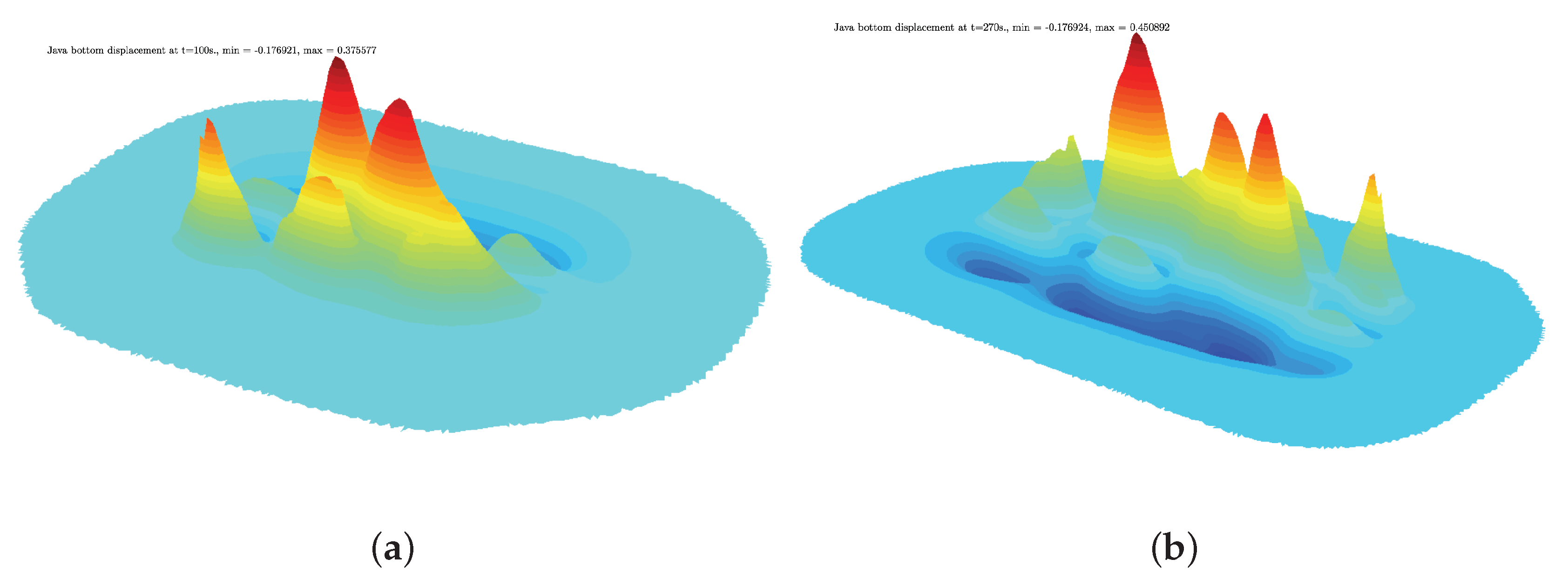
We show, in Figure 8, the bottom displacement at time s and s using our domain adaptation technique. We note that, after building the Okada solution in the passive generation or in the active generation, we can remark that this solution is non-local and decays slowly to zero; that is why, in our domain adaptation technique, we put 0 where the absolute value of the solution is less then m. We make the same thing without adaptive mesh in order to compare the solution using the same initial data.
4. Numerical Simulations
In this section, we study first the rate of convergence of our schemes for the sBBM System (4) with non-dimensional and unscaled variables, i.e., with over a variable bottom in space, which establishes the adequacy of the chosen finite element discretization and the used time marching scheme; for the flat bottom case, we refer to Reference [32], where we use the same technique as in this paper. Then, we simulate the propagation of a wave, that is similar to a real-world tsunami wave generated by an earthquake, in the Mediterranean sea with the BBM–BBM model over a flat bottom. Then, we switch to the Java island region with real variable bottom in space. Finally, we study the active tsunami generation scenario which took place in 2006 near the Java island. In all numerical simulations, we used continuous piecewise linear functions for , u, v, h, and .
4.1. Rate of Convergence
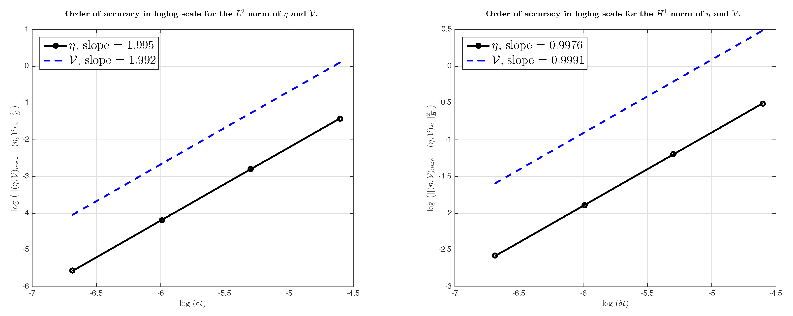
We present the evidence here, following the work done for the 1D case of the BBM–BBM system in Reference [33], that the second order Runge–Kutta time scheme considered for the sBBM variable bottom in space is of order 2. We note that the function is only used for the generation of tsunami wave and, thus, will not be taken into account in the convergence rate test. In this example, we take bi-periodic Boundary Conditions (BC) for , , and on the whole boundary of the square , where , and we consider the following exact solutions:
adding an appropriate function to the right-hand side to make these solutions exact. We measure at time and for and , the following errors
and we end up with the results reported in Table 1. So, the rates for and V is of order ∼2 and the rates for and V is of order ∼1, as shown in the Figure 9, which confirms the convergence of the second-order Runge–Kutta scheme in time for the sBBM system with variable bottom in space.
4.2. Propagation of a Tsunami Wave in the Mediterranean Sea with a Flat Bottom
We simulate here, the propagation of a wave that looks like a tsunami wave generated by an earthquake in the Mediterranean sea with the sBBM System (4) with a flat bottom 1.5 km which is the average depth of the Mediterranean sea. This wave was defined above in the passive generation part of the Section 3 where, in this case, the initial solution is concentrated in the small rectangle and we take these following values: km, km, , , , GPA is the Young’s modulus, is the Poisson’s ratio, m, and the fault depth 10 km. In this example, we will take the fact that the Lamé constants and are given by the formulas and .
An efficient mesh adaptivity algorithm using metrics control adapts the mesh every 50 time steps; we use the standard function (adaptmesh) which is an efficient tool offered by FreeFem++ to efficiently adapt 2D meshes by metrics control [34]; see Reference [35] (Section §3.2) for more details. We also use the following settings: for the step time s, a reflective BC for all the boundary, for the adaptmesh of FreeFem++:
- Th = adaptmesh (Th, uadapt, err = 1.e−7, errg = 1.e − 2, hmin = Dx, iso = true, nbvx = 1e8),
where err: is the interpolation error level inside the geometry, errg: is the interpolation error level on the boundary, hmin: the minimum edge size, iso: forces the metric to be isotropic or not, and nbvx: is the maximum number of vertices allowed in the mesh generator. Finally, for our domain adapt technique: isoadapt , erradapt, , epsadapt. We note that we adapt the mesh around the solution every 100 iterations, i.e., every 10 s, by using uadapt.
In order to compare the results between adaptive mesh generated by FreeFem++, our new domain adaptation technique and without using mesh adaptation, we plot in addition to the free surface elevation in the Figure 5 and Figure 10, the variation of vs. time in Figure 11 at two wave ’gauges’ placed at the positions represented by ⋄ in Figure 3 at right and the mass of the water . Specifically, gauges were placed at the points , . In Figure 12, we represent the comparison between the three methods: full mesh, domain adaptation and FreeFem++ internal mesh adaptivity of the maximum of the propagation of the solution at time s. We also plot the computation time for each adapt mesh, the computation time of the simulation, and the number of degree of freedom in Figure 13. We can see in Figure 11 and Figure 13 that the adaptive mesh generated by FreeFem++ with err is the fastest method but unfortunately it does not preserve the mass invariant . On the other hand, our new domain adaptation technique preserves the mass invariant throughout the simulation with an error of order and an important time computation difference with the one without mesh adaptation which is very promising method for the tsunami wave propagation. For the adaptive mesh generated by FreeFem++ with err = 1.e−7 and errg , we also almost get the mass conservation with an error of order , but we obtain some difference in wave gauge with the full method which is due to the refinement mesh adaptation and the interpolation of the solution, although the computation time is almost the double of the new domain adaptation technique. Thus, we can go faster with our new domain adaptation technique if we can also deduce the mass matrix after cutting the mesh, of course, if the mass matrix does not change along the simulation of the full mesh. This is an outgoing project.
4.3. Propagation of a Tsunami Wave near the Java Island: Passive Generation
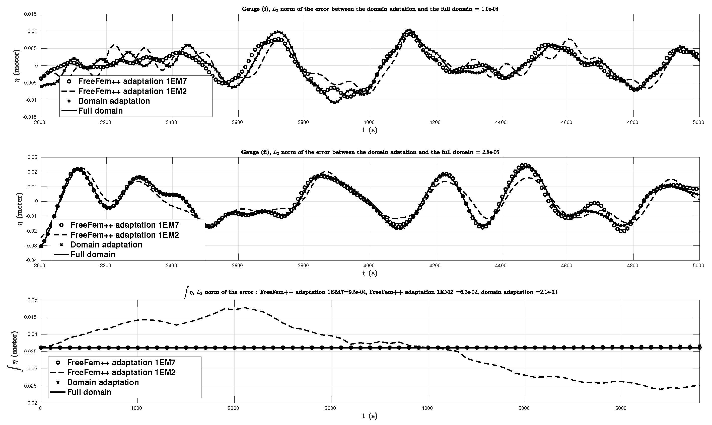
We will take here the same initial data as defined above in the passive generation part of Section 3, we take s as the time step size and we note that, we adapt the mesh after computing the initial data for and then every 50 s by using the following value for the domain adaptation uadapt, isoadapt, erradapt, , epsadapt. We compare here the results between our new domain adaptation technique and without using mesh adaptation. To this end, we plot the free surface elevation in the Figure 14 and Figure 15, the variation of vs. time (in Figure 16) at four numerical wave gauges placed at the following locations: (i) , (ii) , (iii) , and (iv) (see Figure 6 (left)), where (i) is the position of the epicenter. However, because of the large variations of the bottom, shorter waves were generated, especially around Christmas Island (southwest of Java) and around the undersea canyon near the earthquake epicenter.
Finally, we present a comparison of the kinetic, potential and total energies with the full mesh (in Figure 17, top left panel) and with the domain adaptivity method (in Figure 17, top right panel) defined in Reference [36] as follows:
where kg/m is the ocean water density, the number of degrees of freedom (in Figure 17, down left panel), and the computation time of the simulation (in Figure 17, down right panel). We obtain here an error of order between the total energy with domain adaptivity and without any adaptation. We present in Figure 18 the comparison of the maximum of the propagation of the solution between the full and domain adaptivity methods at s.
4.4. Propagation of a Tsunami Wave near the Java Island: Active Generation
For a more realistic case as in the Java 2006 event, we use the active generation in order to model the generation of a tsunami wave as in Reference [10,30]. In this case, we consider zero initial conditions for both the surface elevation and the velocity field, we take s as the time step size, we assume that the bottom described in Section 3 is moving in time, and we note that we adapt the mesh before the end of the generation time s, every three iterations, i.e., every 6 s, by using the following value for the domain adaptation: uadapt, isoadapt, erradapt, , epsadapt, and, then, for s, every 25 iterations, i.e., every 50 s. We compare here only the results between our new domain adaptation technique and without using mesh adaptation. To this end, we plot the free surface elevation in the Figure 19, Figure 20 and Figure 21. However, as in the passive case, because of the large variations of the bottom, shorter waves were generated, especially around the Christmas Island (southwest of Java island) and around the undersea canyon near the earthquake epicenter. We plot the variation of vs time (in Figure 22) at four numerical wave gauges placed at the following locations: (i) , (ii) , (iii) , and (iv) (see Figure 6 (left panel)) where (i) is the position of the epicenter. Finally, we present a comparison of the kinetic, potential and total energies with the full mesh (in Figure 23, top left panel) and with the domain adaptivity method (in Figure 23, top right) defined in (9), the number of the degrees of freedom (in Figure 23, lower left panel) and the computation time of the simulation (in Figure 23, lower right panel). We obtain here an error of order between the total energy with domain adaptivity and without any adaptation. We present in Figure 24 the comparison of the maximum of the propagation of the solution between the full and domain adaptivity method at s.
5. Conclusions and Outlook
In this manuscript, we demonstrated how to discretize a simplified version of the BBM–BBM System (1) using the FEM and dedicated open-source software FreeFem++. The use of this numerical technique was demonstrated in view of applications to tsunami wave modeling [25,37]. The concrete cases of wave propagation in the Mediterranean sea and in Java island region (Indonesia) were considered. The digital computing environment that we developed allows the integration of realistic data (bathymetry and geography) in a relatively simple software framework. The codes used in this study are made freely available for all our readers. Moreover, a novel mesh and domain adaptation technique was proposed to speed-up substantially the computations. The gain in terms of the CPU time after applying this technique can be clearly seen in Figure 23. The accuracy of the ‘accelerated’ solution is more than acceptable to make this technique useful in a variety of tsunami propagation problems. It goes without saying that this technique can be applied to other events and other regions of the world with minimal changes in the provided codes.
Regarding the perspectives of this study, we would like to develop also the parallel version of this code together with the domain adaptation technique to make computations practically faster than the real time tsunami wave propagation. However, we underline that even the current version can be efficiently run even on a modest laptop personal computer. There is another direction that we can see to improve the proposed method. Namely, the idea could be called the ’un-adaptivity’, which consists of removing the portions of the mesh once the wave passed by. This would allow us to keep only the portions of the computational domain where something is going on.
Author Contributions
Conceptualization, G.S. and D.D.; methodology, G.S.; software, G.S.; validation, G.S. and D.D.; investigation, G.S.; writing—original draft preparation, G.S.; writing—review and editing, D.D.; visualization, G.S.; supervision, D.D. All authors have read and agreed to the published version of the manuscript.
Funding
This work has been supported by the French National Research Agency, through Investments for Future Program (ref. ANR-18-EURE-0016—Solar Academy).
Acknowledgments
This work would not be possible without a precious help of Professors Frédéric Hecht, Dimitrios Mitsotakis, and Olivier Pantz. The Authors would like to thank also both Referees for their invaluable comments which allowed us to improve our manuscript.
Conflicts of Interest
The authors declare no conflict of interest.
Abbreviations
The following abbreviations are used in this manuscript:
| 2D | Two-dimensional |
| BBM | Benjamin–Bona–Mahony |
| BC | Boundary Condition |
| FEM | Finite Element Method |
| FreeFem++ | Free Finite Element Method |
| LGPL | GNU Lesser General Public License |
| MOST | Method Of Splitting Tsunami |
| NOAA | National Oceanic and Atmospheric Administration |
| PDE | Partial Differential Equation |
| USGS | United States Geological Survey |
Appendix A. Simplified System Derivation
After integrating by parts, the left hand side of (3) becomes:
and
where is the boundary of the domain . Dealing with the right-hand side of the first equation in System (3), we expand the two complex terms which are multiplied by A and such as:
and
On the other hand, we have:
and, consequently, we deduce the final form of as follows:
References
- Sadaka, G.; Dutykh, D. Adaptive numerical modelling of tsunami wave generation and propagation with FreeFem++. HAL 2020, hal-029125. [Google Scholar] [CrossRef]
- Hecht, F.; Auliac, S.; Pironneau, O.; Morice, J.; Le Hyaric, A.; Ohtsuka, K. FreeFem++ (Manual), 3rd ed.; Université Pierre et Marie Curie: Paris, France, 2007; p. 424. Available online: www.freefem.org (accessed on 1 September 2020).
- Imamura, F. Simulation of wave-packet propagation along sloping beach by TUNAMI-code. In Long-wave Runup Models; Yeh, H., Liu, P.L.F., Synolakis, C.E., Eds.; World Scientific: Singapore, 1996; pp. 231–241. [Google Scholar]
- Titov, V.V.; González, F.I. Implementation and testing of the method of splitting tsunami (MOST) model. In Technical Report ERL PMEL-112, Pacific Marine Environmental Laboratory; NOAA: Seattle, WA, USA, 1997. [Google Scholar]
- Dutykh, D.; Poncet, R.; Dias, F. The VOLNA code for the numerical modeling of tsunami waves: Generation, propagation and inundation. Eur. J. Mech. B/Fluids 2011, 30, 598–615. [Google Scholar] [CrossRef] [Green Version]
- Khakimzyanov, G.S.; Dutykh, D.; Mitsotakis, D.; Shokina, N.Y. Numerical simulation of conservation laws with moving grid nodes: Application to tsunami wave modelling. Geosciences 2019, 9, 197. [Google Scholar] [CrossRef] [Green Version]
- Boussinesq, J.V. Théorie généale des mouvements qui sont propagés dans un canal rectangulaire horizontall. C. R. Acad. Sci. Paris 1871, 73, 256–260. [Google Scholar]
- Wu, T.Y. Long Waves in Ocean and Coastal Waters. J. Eng. Mech. 1981, 107, 501–522. [Google Scholar]
- Dias, F.; Dutykh, D.; O’Brien, L.; Renzi, E.; Stefanakis, T. On the Modelling of Tsunami Generation and Tsunami Inundation. Procedia IUTAM 2014, 10, 338–355. [Google Scholar] [CrossRef]
- Dutykh, D.; Mitsotakis, D.; Gardeil, X.; Dias, F. On the use of the finite fault solution for tsunami generation problems. Theor. Comput. Fluid Dyn. 2013, 27, 177–199. [Google Scholar] [CrossRef] [Green Version]
- Guesmia, M.; Heinrich, P.H.; Mariotti, C. Numerical simulation of the 1969 Portuguese tsunami by a finite element method. Nat. Hazards 1998, 17, 31–46. [Google Scholar] [CrossRef]
- Lynett, P.J.; Borrero, J.C.; Liu, P.L.F.; Synolakis, C.E. Field Survey and Numerical Simulations: A Review of the 1998 Papua New Guinea Tsunami. Pure Appl. Geophys. 2003, 160, 2119–2146. [Google Scholar] [CrossRef]
- Mitsotakis, D.E. Boussinesq systems in two space dimensions over a variable bottom for the generation and propagation of tsunami waves. Math. Comp. Simul. 2009, 80, 860–873. [Google Scholar] [CrossRef] [Green Version]
- Whitham, G.B. Linear and Nonlinear Waves; John Wiley & Sons, Inc.: Hoboken, NJ, USA, 1999; p. 656. [Google Scholar] [CrossRef]
- Stoker, J.J. Water Waves: The Mathematical Theory with Applications; John Wiley and Sons, Inc.: Hoboken, NJ, USA, 1992; p. 600. [Google Scholar] [CrossRef]
- Peregrine, D.H. Calculations of the development of an undular bore. J. Fluid Mech. 1966, 25, 321–330. [Google Scholar] [CrossRef]
- Peregrine, D.H. Long waves on a beach. J. Fluid Mech. 1967, 27, 815–827. [Google Scholar] [CrossRef]
- Løvholt, F.; Pedersen, G. Instabilities of Boussinesq models in non-uniform depth. Int. J. Num. Meth. Fluids 2009, 61, 606–637. [Google Scholar] [CrossRef]
- Liang, Q.; Hou, J.; Amouzgar, R. Simulation of Tsunami Propagation Using Adaptive Cartesian Grids. Coast. Eng. J. 2015, 57, 1550016. [Google Scholar] [CrossRef]
- Popinet, S. A vertically-Lagrangian, non-hydrostatic, multilayer model for multiscale free-surface flows. J. Comp. Phys. 2020, 418, 109609. [Google Scholar] [CrossRef]
- Dias, F.; Dutykh, D. Dynamics of tsunami waves. In Extreme Man-Made and Natural Hazards in Dynamics of Structures; Ibrahimbegovic, A., Kozar, I., Eds.; Springer: Dordrecht, The Netherlands, 2007; pp. 35–60. [Google Scholar] [CrossRef] [Green Version]
- Dougalis, V.A.; Mitsotakis, D.E.; Saut, J.C. On initial-boundary value problems for a Boussinesq system of BBM-BBM type in a plane domain. Discret. Contin. Dyn. Syst. 2009, 23, 1191–1204. [Google Scholar] [CrossRef]
- Khakimzyanov, G.; Dutykh, D. Long Wave Interaction with a Partially Immersed Body. Part I: Mathematical Models. Commun. Comput. Phys. 2020, 27, 321–378. [Google Scholar] [CrossRef]
- Dutykh, D.; Dias, F. Water waves generated by a moving bottom. In Tsunami and Nonlinear Waves; Kundu, A., Ed.; Springer: Berlin/Heidelberg, Germany, 2007; pp. 65–95. [Google Scholar] [CrossRef] [Green Version]
- Dutykh, D. Mathematical Modelling of Tsunami Waves. Ph.D. Thesis, École Normale Supérieure de Cachan, Cachan, France, 2007. [Google Scholar]
- Okada, Y. Surface deformation due to shear and tensile faults in a half-space. Bull. Seismol. Soc. Am. 1985, 75, 1135–1154. [Google Scholar]
- Okada, Y. Internal deformation due to shear and tensile faults in a half-space. Bull. Seismol. Soc. Am. 1992, 82, 1018–1040. [Google Scholar]
- Kervella, Y.; Dutykh, D.; Dias, F. Comparison between three-dimensional linear and nonlinear tsunami generation models. Theor. Comput. Fluid Dyn. 2007, 21, 245–269. [Google Scholar] [CrossRef] [Green Version]
- Dutykh, D.; Dias, F.; Kervella, Y. Linear theory of wave generation by a moving bottom. Comptes Rendus Math. 2006, 343, 499–504. [Google Scholar] [CrossRef] [Green Version]
- Dutykh, D.; Mitsotakis, D.; Chubarov, L.B.; Shokin, Y.I. On the contribution of the horizontal sea-bed displacements into the tsunami generation process. Ocean Model. 2012, 56, 43–56. [Google Scholar] [CrossRef] [Green Version]
- Hammack, J. A note on tsunamis: Their generation and propagation in an ocean of uniform depth. J. Fluid Mech. 1973, 60, 769–799. [Google Scholar] [CrossRef] [Green Version]
- Sadaka, G. Solution of 2D Boussinesq systems with FreeFem++: The flat bottom case. J. Numer. Math. 2012, 20, 303–324. [Google Scholar] [CrossRef] [Green Version]
- Senthilkumar, A. On the influence of wave reflection on shoaling and breaking solitary Waves. Proc. Est. Acad. Sci. 2016, 65, 414–430. [Google Scholar] [CrossRef]
- Hecht, F. New development in Freefem++. J. Numer. Math. 2012, 20, 251–266. [Google Scholar] [CrossRef]
- Rakotondrandisa, A.; Sadaka, G.; Danaila, I. A finite-element toolbox for the simulation of solid-liquid phase-change systems with natural convection. Comput. Phys. Commun. 2020, 253, 107188. [Google Scholar] [CrossRef] [Green Version]
- Dutykh, D.; Dias, F. Energy of tsunami waves generated by bottom motion. Proc. R. Soc. Lond. A 2009, 465, 725–744. [Google Scholar] [CrossRef] [Green Version]
- Sadaka, G. Etude mathématique et numérique d’équations d’ondes aquatiques amorties. Ph.D. Thesis, Université de Picardie Jules Verne, Amiens, France, 2011. [Google Scholar]
Figure 1.
The sketch of the physical domain .

Figure 2.
Domain adaptation technique step: (a): initial solution, (b): the solution unew mapped from the initial solution over a mesh augmented by epsadapt, (c): the new Heaviside function unewadapt which have a value of 1 (the red part in the figure) if erradapt and 0 otherwise, (d): the function usmadapt which is the smoothness of the unewadapt, (e): the new Heaviside function ufinal which have a value of 1 (the red part in the figure) if erradapt and 0 otherwise, (f): mapped of the initial solution to the final domain adapted.

Figure 3.
Left (a): the mesh around the Crete island. Right (b): the place of ⋄: wave gauge and ⋆: epicenter.
Figure 3.
Left (a): the mesh around the Crete island. Right (b): the place of ⋄: wave gauge and ⋆: epicenter.

Figure 4.
Left (a): Bathymetry downloaded from the National Oceanic and Atmospheric Administration (NOAA) website, (min m and max m). Right (b): smoothed bathymetry with in (8), (min m and max m).
Figure 4.
Left (a): Bathymetry downloaded from the National Oceanic and Atmospheric Administration (NOAA) website, (min m and max m). Right (b): smoothed bathymetry with in (8), (min m and max m).

Figure 5.
The mesh and the numerical isoline of the solution at s, with the full method at the left panel (a), the domain adaptive method at the center panel (b) and the FreeFem++ adaptation with err = 1.e−7 at the right panel (c).
Figure 5.
The mesh and the numerical isoline of the solution at s, with the full method at the left panel (a), the domain adaptive method at the center panel (b) and the FreeFem++ adaptation with err = 1.e−7 at the right panel (c).

Figure 6.
Left panel (a): Surface projection of the fault’s plane and the mesh around, ⋄: wave gauge, ⋆: epicenter. Right panel (b): the 14-th Okada solution (min m, max m ).
Figure 6.
Left panel (a): Surface projection of the fault’s plane and the mesh around, ⋄: wave gauge, ⋆: epicenter. Right panel (b): the 14-th Okada solution (min m, max m ).

Figure 7.
Geometry of the source model (a) and the initial solution for ((b), min m, max m).

Figure 8.
Bottom displacement at s ((a), min m, max m) and at s; ((b), min m, max m).

Figure 9.
Rate of convergence for Benjamin–Bona–Mahony (sBBM) system (4) with variable bottom in space.
Figure 9.
Rate of convergence for Benjamin–Bona–Mahony (sBBM) system (4) with variable bottom in space.

Figure 10.
The solution at s, with the full method at the left panel (a), the domain adaptive method at the center panel (b) and the FreeFem++ adaptation with err at the right panel (c) (min m, max m, for the three case).
Figure 10.
The solution at s, with the full method at the left panel (a), the domain adaptive method at the center panel (b) and the FreeFem++ adaptation with err at the right panel (c) (min m, max m, for the three case).

Figure 11.
Comparison between the three methods: full, FreeFem++ adaption with err and err and the domain adaptation of the free surface elevations (in meters) vs. time (in seconds), computed numerically at two wave gauges (up and middle) and of the mass conservation (down).
Figure 11.
Comparison between the three methods: full, FreeFem++ adaption with err and err and the domain adaptation of the free surface elevations (in meters) vs. time (in seconds), computed numerically at two wave gauges (up and middle) and of the mass conservation (down).

Figure 12.
Comparison between the three method full (a), domain adaptation (b) and adaptive mesh generated by FreeFem++ with err (c) of the maximum of the propagation of the solution of a tsunami wave in the Mediterranean sea for s (min m, max m, for three cases).
Figure 12.
Comparison between the three method full (a), domain adaptation (b) and adaptive mesh generated by FreeFem++ with err (c) of the maximum of the propagation of the solution of a tsunami wave in the Mediterranean sea for s (min m, max m, for three cases).

Figure 13.
Comparison between the three methods: full, FreeFem++ adaption with err and err and domain adaptation of the computation time of each mesh/domain adaptation (left), the number of degrees of freedom (middle), and the computation time of the simulation (right).
Figure 13.
Comparison between the three methods: full, FreeFem++ adaption with err and err and domain adaptation of the computation time of each mesh/domain adaptation (left), the number of degrees of freedom (middle), and the computation time of the simulation (right).

Figure 14.
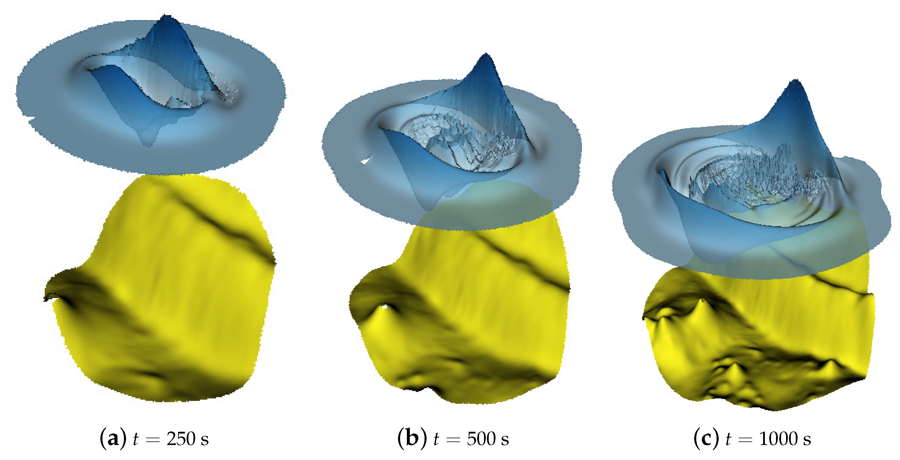
Passive generation: the bottom together with the free surface elevation at different instances of time obtained with the proposed domain adaptivity method.
Figure 14.
Passive generation: the bottom together with the free surface elevation at different instances of time obtained with the proposed domain adaptivity method.

Figure 15.
Passive generation: comparison between the bottom and the free surface elevation at s between the domain adaptation method and the full mesh.
Figure 15.
Passive generation: comparison between the bottom and the free surface elevation at s between the domain adaptation method and the full mesh.

Figure 16.
Passive generation: comparison between the two methods the full one and domain adaptivity of the free surface elevations (in meters) vs. time (in seconds), computed numerically at four wave gauges where the gauge (i) corresponds to the epicenter.
Figure 16.
Passive generation: comparison between the two methods the full one and domain adaptivity of the free surface elevations (in meters) vs. time (in seconds), computed numerically at four wave gauges where the gauge (i) corresponds to the epicenter.

Figure 17.
Passive generation: comparison between the two methods the full one and domain adaptivity of the kinetic, potential and total energies, the number of degrees of freedom, and the computation time of the simulation.
Figure 17.
Passive generation: comparison between the two methods the full one and domain adaptivity of the kinetic, potential and total energies, the number of degrees of freedom, and the computation time of the simulation.

Figure 18.
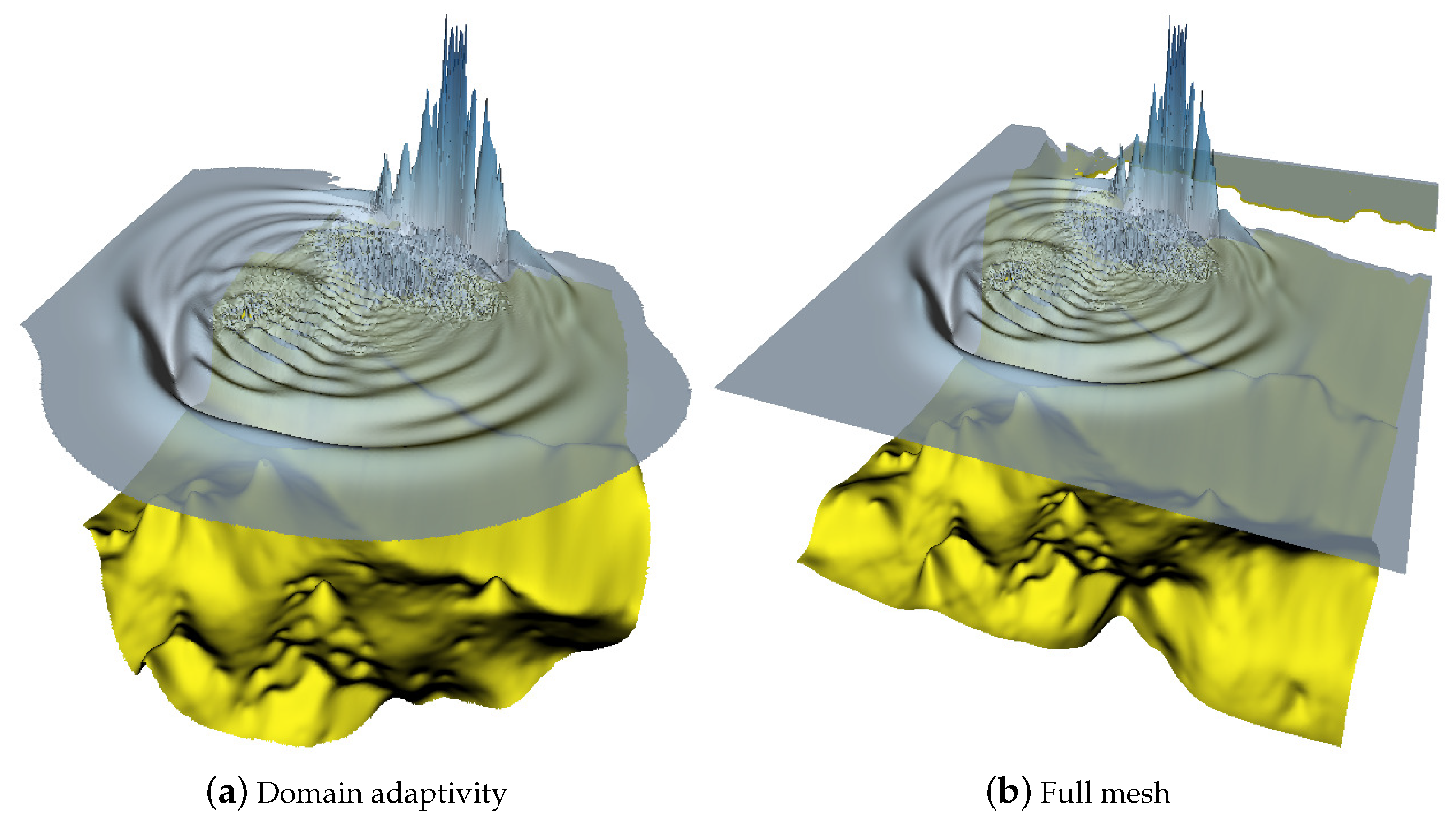
Passive generation: comparison between the maximum of the solution at s, with the domain adaptivity method (left panel) and with the full one (right panel).
Figure 18.
Passive generation: comparison between the maximum of the solution at s, with the domain adaptivity method (left panel) and with the full one (right panel).

Figure 19.
Active generation: the bottom and the free surface elevation computed with the domain adaptivity method.
Figure 19.
Active generation: the bottom and the free surface elevation computed with the domain adaptivity method.

Figure 20.
Active generation: the bottom and the free surface elevation computed with the domain adaptivity method.
Figure 20.
Active generation: the bottom and the free surface elevation computed with the domain adaptivity method.

Figure 21.
Active generation: comparison between the bottom and the free surface elevation at s between the domain adaptivity method and the full mesh.
Figure 21.
Active generation: comparison between the bottom and the free surface elevation at s between the domain adaptivity method and the full mesh.

Figure 22.
Active generation: comparison between the two methods (the full one and domain adaptivity) of the free surface elevations (in meters) vs. time (in seconds), computed numerically at four wave gauges where the gauge (i) correspond to the epicenter.
Figure 22.
Active generation: comparison between the two methods (the full one and domain adaptivity) of the free surface elevations (in meters) vs. time (in seconds), computed numerically at four wave gauges where the gauge (i) correspond to the epicenter.

Figure 23.
Active generation: comparison between the two methods (the full one and the domain adaptivity) of the kinetic, potential and total energies, the number of degrees of freedom, and the computation time of the simulation.
Figure 23.
Active generation: comparison between the two methods (the full one and the domain adaptivity) of the kinetic, potential and total energies, the number of degrees of freedom, and the computation time of the simulation.

Figure 24.
Active generation: comparison between the maximum of the solution at s, with the domain adaptivity method (a) and with the full one (b).
Figure 24.
Active generation: comparison between the maximum of the solution at s, with the domain adaptivity method (a) and with the full one (b).


Table 1.
norm of the error for and V.
| N | Rate | Rate | Rate | Rate | |||||
|---|---|---|---|---|---|---|---|---|---|
| 0.24145 | - | 1.10773 | - | 0.60317 | - | 1.62575 | - | ||
| 0.06078 | 1.990 | 0.28016 | 1.983 | 0.30196 | 0.998 | 0.81276 | 1.000 | ||
| 0.01524 | 1.996 | 0.07038 | 1.993 | 0.15119 | 0.998 | 0.40696 | 0.999 | ||
| 0.00381 | 1.999 | 0.01760 | 1.999 | 0.07578 | 0.998 | 0.20355 | 0.999 |
© 2020 by the authors. Licensee MDPI, Basel, Switzerland. This article is an open access article distributed under the terms and conditions of the Creative Commons Attribution (CC BY) license (http://creativecommons.org/licenses/by/4.0/).
Share and Cite
MDPI and ACS Style
Sadaka, G.; Dutykh, D. Adaptive Numerical Modeling of Tsunami Wave Generation and Propagation with FreeFem++. Geosciences 2020, 10, 351. https://doi.org/10.3390/geosciences10090351
AMA Style
Sadaka G, Dutykh D. Adaptive Numerical Modeling of Tsunami Wave Generation and Propagation with FreeFem++. Geosciences. 2020; 10(9):351. https://doi.org/10.3390/geosciences10090351
Chicago/Turabian StyleSadaka, Georges, and Denys Dutykh. 2020. "Adaptive Numerical Modeling of Tsunami Wave Generation and Propagation with FreeFem++" Geosciences 10, no. 9: 351. https://doi.org/10.3390/geosciences10090351
Note that from the first issue of 2016, this journal uses article numbers instead of page numbers. See further details here.