Inverse Infiltration Modeling of Dike Covers Made of Dredged Material Using PEST and AMALGAM

Department Geotechnics and Coastal Engineering, Universität Rostock, Justus-von-Liebig-Weg 6, 18059 Rostock, Germany
*
Author to whom correspondence should be addressed.
Geosciences 2021, 11(2), 41; https://doi.org/10.3390/geosciences11020041
Submission received: 20 October 2020
/
Revised: 8 January 2021
/
Accepted: 10 January 2021
/
Published: 21 January 2021
(This article belongs to the Section Hydrogeology)
Abstract
:A variety of studies recently proved the applicability of different dried, fine-grained dredged materials as replacement material for erosion-resistant sea dike covers. In Rostock, Germany, a large-scale field experiment was conducted, in which different dredged materials were tested with regard to installation technology, stability, turf development, infiltration, and erosion resistance. The infiltration experiments to study the development of a seepage line in the dike body showed unexpected measurement results. Due to the high complexity of the problem, standard geo-hydraulic models proved to be unable to analyze these results. Therefore, different methods of inverse infiltration modeling were applied, such as the parameter estimation tool (PEST) and the AMALGAM algorithm. In the paper, the two approaches are compared and discussed. A sensitivity analysis proved the presumption of a non-linear model behavior for the infiltration problem and the Eigenvalue ratio indicates that the dike infiltration is an ill-posed problem. Although this complicates the inverse modeling (e.g., termination in local minima), parameter sets close to an optimum were found with both the PEST and the AMALGAM algorithms. Together with the field measurement data, this information supports the rating of the effective material properties of the applied dredged materials used as dike cover material.
1. Introduction
In engineering practice, numerical simulations of water infiltration are a component of the design of flood protection dikes. The stability of the dike cross-section is affected by pore water pressures inside the dike body. Therefore, infiltration analysis is required by national (German) and international standards and regulations for sea and estuary dikes as well as river dikes [1,2,3,4]. This analysis is usually performed using hydraulic simulations in the steady and transient state to determine problematic hydraulic loads which may lead to failure, e.g., corresponding to the failure modes provided in the EC7 [5]. From these considerations, the desired material properties of individual construction elements are chosen in accordance with the applied directives and material availabilities. In the design procedures, partial safety factors are used to account for the involved material uncertainties. The predicted or predefined properties of these material properties are checked on the construction site by comprehensive laboratory and field tests.
Generally, dike cover materials are of low hydraulic conductivity (Ks), to reduce flow into and through the dike body. However, Temmler [6] observed high infiltration rates (1 × 10⁻⁶ ms−1–6 × 10⁻⁵ ms−1) on dike covers along German North Sea and estuary dikes despite their low Ks values determined in the laboratory prior to installation. Correlations between the basic geotechnical properties and the Ks values were not found in the study, but it was supposed that the Ks correlates with the soil texture. Heyer and Schmutterer [7] recommend permittivity values of dike sealing layers of ψ < 1 × 10⁻⁸ L/s, concluding that if the permittivity considerably exceeds this value, the risk probability of stability failure generally rises. Similar processes were observed with processed dredged materials used as replacement materials for dike covers in Rostock, Germany, where large-scale field tests were performed to investigate their performance in field application [8].
A vast amount of sediment is being dredged all around the world, e.g., during maintenance works in harbors and rivers. Most of the dredged sediments worldwide are sand, which is usually relocated in the water body. Materials with lager fine fractions and/or contamination, however, are restricted from relocation, and thus need to be put on land for beneficial use or disposal, depending on their level of contamination. Non-contaminated materials have been used as construction material, e.g., in landfill restoration, in filling former mining areas or in landscaping and agriculture. The application of fine-grained dredged materials to replace dike cover material has a comparatively short history. In Germany, practical experiments with fine-grained dredged materials were made on the dike “CT4- North Dike” in Bremerhaven [9] and on a test field in Hamburg using processed (low-contamination) dredged materials from the METHA (mechanical treatment and dewatering of harbor sediments) plant [10,11]. Further practical experiments with the installation of dredged materials were made in the Netherlands and Belgium, e.g., on the Schelde River [12]. With only very few projects realized, there is still a lack of knowledge about the materials’ infiltration behavior and hydraulic material properties in the field. Laboratory work and several field experiments indicate their suitability in the construction of Baltic sea dikes, particularly due to their high erosion resistance. Physical flood simulation tests showed that infiltration is much higher than predicted, even when applying a factor of one to two orders of magnitude to the laboratory values. This leads to increased phreatic lines inside the dike body, and drainage discharge from the land-side toe [13].
For a wider application of dredged material in dike construction, the hydraulic performance of the materials needs to be quantified. This involves reliable values for the saturated and unsaturated hydraulic conductivities in field application. The finite-element software Feflow [14] was used to simulate the infiltration processes and to quantify the material properties based on field measurement data for the Rostock research dike, which was built and investigated within the European cooperation project DredgDikes [8]. It has been shown by [15] and [16] that such simulations are suitable in order to model the natural process of dike infiltration. In this study, techniques of inverse model calibration with the data from field experiments are applied, which are frequently used in geo-hydrology [17]. Both the application of the parameter estimation tool (PEST) [18,19,20] and the multi-algorithm, genetically adaptive multi-objective method AMALGAM [21] have been tested regarding their suitability for the parameter identification and the quantification in focus.
The purpose of this study is to find an effective method to evaluate the hydraulic material properties of the different cross-section layouts of the Rostock research dike in field performance, based on the 45 observation data sets obtained by flood simulation tests performed between 2013 and 2016. Numerical model limitations (e.g., over-parameterization, model complexity, model consistency) are discussed with regard to model deviations, a sensitivity analysis and the accuracy of this ill-posed problem.
2. Materials and Methods
2.1. Physical Model—The Rostock Research Dike
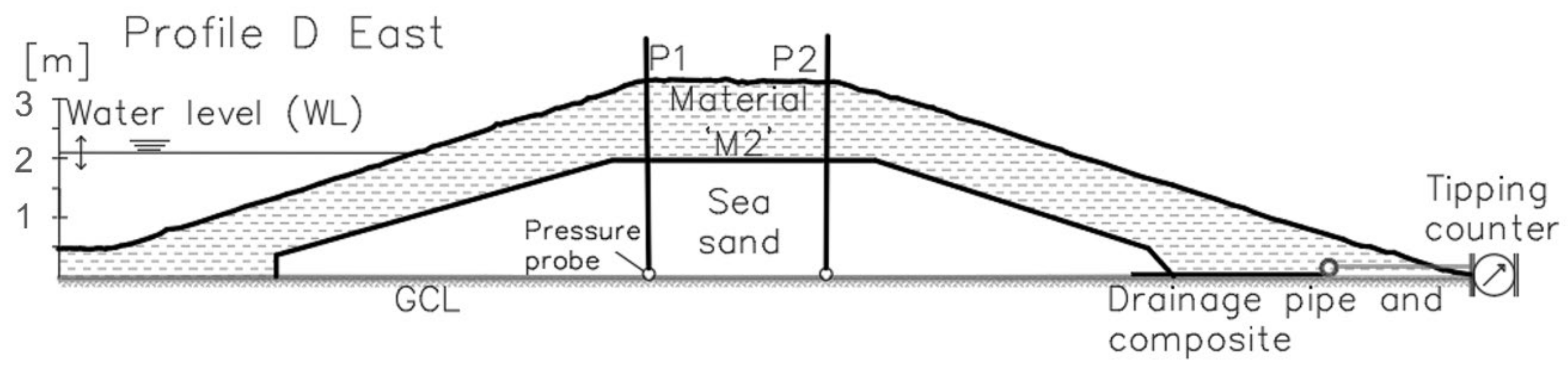
The Rostock research dike is made of different dried, fine-grained dredged materials with high organic content. The construction is approximately 145 m long and consists of two parallel dikes, between which water can be filled for hydraulic tests, e.g., to study the development of the phreatic line while maintaining a flood water level. The research dike is divided into different cross-sections with different material combinations. Underneath the dike, a geosynthetic clay liner (GCL) has been installed on the subbase as the lower hydraulic boundary condition. This study focuses on one of the material combinations, namely cross-section D, consisting of a stable body made of a poorly graded sea sand “S” and a cover layer of approximately 1 m thickness, made of dredged material, “M2” (Figure 1). The cover layer was installed and compacted in layers of 0.30 m, using the caterpillar tracks for compaction perpendicular to the longitudinal axis [22]. A drainage pipe has been installed inside the sand core at the land-side toe to collect infiltrating water. For better drainage performance, the pipe was wrapped and extended with a drainage composite (Enkadrain®; Low & Bonar Ltd., the Netherlands). The drainage pipe leads the discharge to a tipping counter, where it was recorded constantly during the experiment. Two piezometer pipes (P1, P2) have been installed in the center, and enable local observations on the phreatic line (hydraulic head data).
2.2. Basic Numerical Model
Based on the geometry of cross-section D, derived from geodetic survey and excavation data, three variations of Feflow finite element models with increasing complexity (each with a total number of 487 nodes) are generated to solve the Richards equation numerically and to simulate the unsaturated and saturated infiltration in a vertical-slice 2D cross-section. The model fit (the objective) is expressed by the weighted sum of squared residuals (wSSR) (Equation (2)) and the mean square error (MSE) (Equation (3)) (see Section 2.6 and Section 2.7), which are calculated from observation and simulation data and should result in zero at the global minimum for a well-fitted model. The model variations need several runs to investigate the effects of critical parameters (e.g., effects of anisotropy or properties of the drainage element), to find proper settings (e.g., weighting strategy, determination criteria, type of algorithm), and to evaluate minima solutions. Subsequently, the AMALGAM algorithm is applied as a second approach to verify the results.
The relevant parameters to be adjusted are identified as follows: the pore void ratio n (1), the saturated hydraulic conductivity Ks (ms−1), and the drainage element parameter D (m2), which is described by a cross-section area of discrete pipe flow elements formulated with the Hagen–Poiseuille law.
There is also an option to adjust the anisotropy parameter A [1] of the flow parameters (quotient of the vertical and horizontal hydraulic conductivity coefficients). The dredged material was installed in layers, as explained above [22], and even though significant effects are not expected, the presence of an anisotropic behavior of the Ks value in the plane of the cover layer and perpendicular to the surface is possible. However, the implementation of such factors might cause interdependencies in combination with the Ks-values and other model parameters. Usually, the shape of the phreatic line corresponds to the chosen parameter of the drainage element, parameter D, the Ks-values and the pore void ratio. Independent of these parameters, the anisotropy affects the phreatic line directly, and therefore, anisotropy factors need to be discussed separately.
If macro pores are present in the dike cover layer (e.g., due to desiccation cracks, bioturbation or low compaction), the permittivity is primarily a function of the macro pore aperture, the connectivity, the tortuosity and the length of these macro pores [23]. The infiltration then needs to be calculated with dual porosity approaches because the matrix flow becomes negligibly small for cohesive soil materials with low permeability [24,25]. This improves the model fitting (e.g., regarding suction pressure data), and may indicate the nature of infiltration more appropriately; the model, however, becomes much more complex (increasing computation effort, numerical instability and ill-posedness). Therefore, the application of a dual porosity approach is not suitable for the inverse calibration problem studied. In this study, the infiltration is rather treated as an effective matrix flow (summarizing macro pore flow and matrix flow in one property).
The VanGenuchten–Mualem formulation [26] is used to model the unsaturated flow. The respective fitting parameters (VGSS, VGSR, VGα, VGn) are estimated in the model optimization, because the model accuracy is usually not much improved by fitting the soil water retention curve (SWRC) on laboratory data [15]. In this case, both the SWRC (assuming a unimodal pore size distribution) and the macro pores will be summarized in one effective property. These model simplifications considerably decrease the model consistency, and should therefore be included in the model evaluation.
2.3. Material Properties
The dike core of the research dike is made of sea sand, S, classified as a poorly-graded fine sand. The cover layer consists of the dredged material M2, which is classified as a fine-grained sandy silt with high fractions of total organic content (TOC). The geotechnical and geo-hydraulic properties of the materials were determined in the laboratory by Saathoff et al. [8]. A selection of parameters relevant for this study are summarized in Table 1.
The saturated hydraulic conductivities (Ks) have been determined in laboratory tests with both disturbed and undisturbed soil samples, varying in more than two orders of magnitude. The disturbed samples were prepared in a Proctor compaction apparatus with optimal density. The dredged materials studied have a particular aggregate structure with larger and comparably stable agglomerates, which may be destroyed during Proctor compaction. The measured dry densities in the field are below Proctor density (degree of compaction approximately 75–85%) due to the high natural water contents of the materials during installation.
To supplement the laboratory analysis, eight infiltration tests were performed on the eastern slope of cross-section D using the double ring infiltration method [27]. The test sites were located at the bottom, the center and the top of the slope on both sides of the middle section and 0.10–0.30 m below the surface level. The results are summarized in Figure 2. The tests Ia and Ib were both performed in location I (bottom, right side) in one another’s immediate vicinity, in order to check for local variances. Test Vb (in location V, top, right side) was conducted directly after test Va, at a depth of 0.50 m below the surface, to indicate possible variance with increasing depth.
After the infiltration tests, gypsum tracer was used to detect desiccation cracks at the same plot and the subsoil was analyzed after another 24 h regarding the tracer distribution in the vertical profile.
The measured infiltration rates range from 2.3 × 10⁻⁵ ms−1 to 1 × 10⁻⁴ ms−1, indicating the behavior of a permeable material [28]. Correlations of the different locations to any relevant parameters could not be determined. The narrow margin of the results indicates that the infiltration is not significantly affected by desiccation cracks, although some small cracks were observed (Figure 3b). The infiltration rate in Vb (deeper level) is not significantly lower compared to the other locations. The values are within a common variance of soil inhomogeneity.
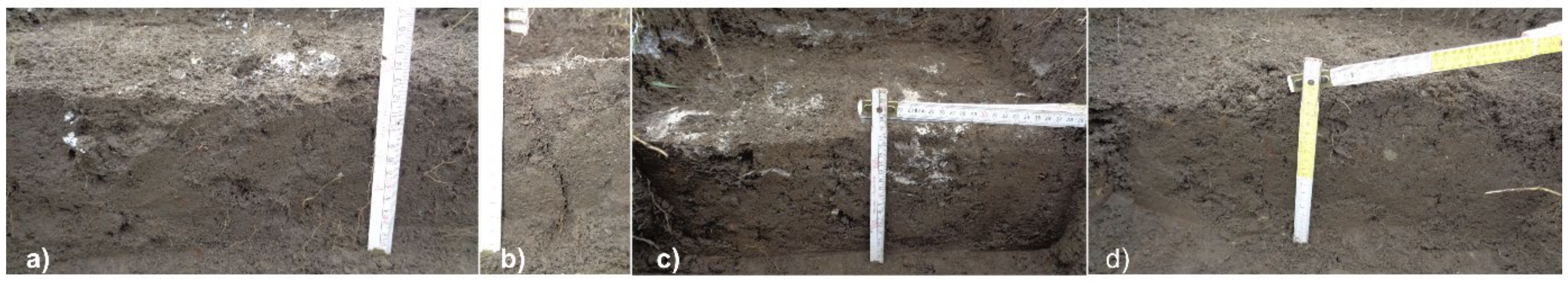
In all excavated soil profiles, large pore voids and plant roots have been found (Figure 3). Small desiccation cracks (aperture < 3 mm) were observed in location IV (Figure 3b); however, they were not detected by the gypsum tracer test. It must be concluded that the entire surface of the cover layer is textured. The infiltration rates are high all along the surface up to a depth of at least 0.50 m, and this is not primarily caused by individual desiccation cracks or bioturbation as initially assumed.
2.4. Observation Data
Several physical experiments have been conducted on the Rostock research dike in order to investigate the dike stability and the material behavior under hydraulic stress. Tensiometers were used to measure the desorption and absorption characteristics of the dike cover material in the infiltration area at different depths. The moisture content was recorded using frequency domain reflectometry (FDR) probes near to the subbase and inside the dike core. A permanent pressure gauge was used in piezometer P1 to observe local changes on the hydraulic head. These data were complemented by discontinuous manual water level measurements in the piezometer P2. The drainage discharge was recorded with a tipping counter at the outlet of the drainage pipe [13].
The FDR data (at the dike bottom) show permanent high saturation values and no significant reaction in the flood experiments [13]. The tensiometer data, on the other hand, highly depend on local inconsistencies of the soil texture. Inverse modeling of these data would therefore necessarily include macro pore simulation [25]. Therefore, the available FDR and tensiometer data are not used for the model calibration in this study. Only the time series of the hydraulic head and the drainage discharge (recorded from 26th June to 7th July 2013) are appropriate for the model calibration to determine the effective material properties (Figure 4).
2.5. Model Set Up and Variations
The flow model is set up in the commercial finite element modelling software Feflow. The general cross-section of Figure 1 is used. The governing boundary condition (BC) on the left model edge is formulated by a Dirichlet BC using the recorded water level (WL) as time series. An unconstrained BC is used for the right model edge and allows the computation of undefined seepage conditions that enables a zero-pressure condition for the drainage discharge. The geosynthetic clay liner (GCL) is modeled by an impervious layer using a Neumann’s BC. The drainage component on the right side is represented by a pipe flow discrete feature element (Hagen-Poiseuille).
The optimization procedure involves the discussion of different model variations, because they do the following:
- -
- allow different physical interpretations;
- -
- are needed to look at the problems of over- and under-parameterization;
- -
- help to discuss the ability of global optimization and the quality of the fitting algorithm.
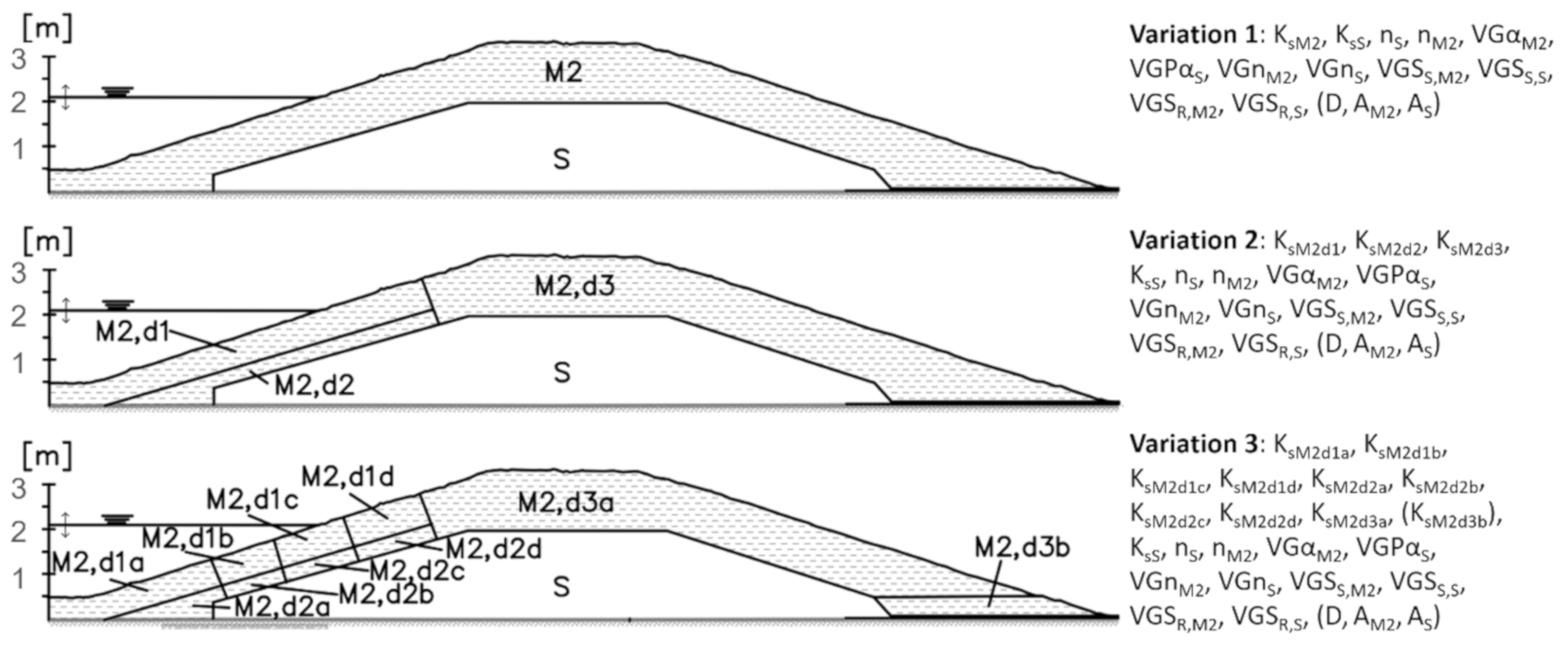
An overview of the three variations is provided in Figure 5. It contains the definitions of zones (cover layer, sand core, drainage element) and sections with different soil properties in three dike cross-sections with different complexities, and the respective fitting parameters to be adjusted, with a certain nomenclature.
Variation 1 is a simple model with constant material properties in each of the three zones (S, M2, drainage), requiring few calibration parameters. In variation 2, the infiltration area is subdivided into two separate sections to account for vertical variances in the hydraulic conductivity (e.g., caused by plant roots, compaction differences, and desiccation cracks). In variation 3, the area of infiltration is divided into eight sections in order to enable vertical and horizontal variances in the hydraulic conductivity. An optional section “M2, d3b” is introduced to enable additional adjustments at the right model edge. In all three variations, the pore void ratio, the VanGenuchten and the anisotropy parameters are kept constant within the zones and the respective sections, considering the material properties of M2 and S.
2.6. FePEST/PEST Optimization
The applied PEST algorithm (implemented in FEFLOW, therefore FePEST) is a nonlinear iterative optimization tool that follows the Gauss–Levenberg–Marquardt algorithm (GLMA) to minimize the objective function φ to a target that should be zero. At the beginning of each iteration step and based on the current best parameter set, the relationship between the model parameters and the model-generated observation data is linearized using a Taylor expansion. Subsequently, the derivatives (sensitivities) of all observations with respect to all parameters are calculated by numerical differentiation (Equation (1)) and are stored in Jacobian matrix elements.
where
- φ0 = objective of the current iteration
- P0 = parameter of the current iteration
- φ = new objective
- P = adjusted parameter
To do so, one of the parameters is adjusted and the change in the objective is observed. A parameter upgrade vector is calculated corresponding to the relative parameter changes and improved parameter sets are proposed. Implementing these new parameter sets into the Feflow model and running the model several times, the changes and improvements in the objective function of the current iteration step are compared to those of the previous iteration. The iteration procedure is repeated until one of the user-specified fixed termination criteria is met [19].
In PEST, the objective function (OBF) is calculated by the weighted sum of squared residuals (wSSR) (Equation (2)) [29].
where
- φ = objective function (OBF)
- wi = weight factor
- hiobs = time series of the observation data (field measurement data)
- hisim = time series of the simulation data
- i = 1…n: the index number of the time series value pairs
With respect to the available measurement data for the current optimization problem and due to their differing physical meaning, the hydraulic head data are referred to group φHH, and the discharge data are referred to group φQ, in which a weighting factor of 10 was chosen to take account of the scaling nature of the discharge data. Both groups are summed up to the major objective function.
The independent fitting tool-set PEST is a well-documented, non-commercial software. It provides many different tools (e.g., different regularization methods, sensitivity and uncertainty analysis, stability tests), and has a variety of features useful for model calibration. Using the FePEST tool as a graphical user interface linking the Feflow model with PEST, the fitting becomes very robust and is comparatively easy to handle. However, for complex problems, the result of the PEST optimization can be strongly dependent on the choice of the termination criteria, the weighting factors, and the chosen initial parameters. PEST only handles one objective function, which is computed for a variety of time series. This generally increases the presence of local minima and possibly makes the model fitting unstable. Although PEST seems to generally work for the model calibration of the studied problem, with the drawback of stability and convergence problems, a second algorithm is applied, using multi-objective optimization and a global search to find the minimum.
2.7. AMALGAM Optimization
The AMALGAM method [21] is based on evolutionary search algorithms for mathematical optimization. In recent years, evolutionary search algorithms have been applied to solve many different environmental optimization problems. According to Efstratiadis and Koutsoyiannis [30], these methods can be very efficient in solving minimizing problems such as the one under study. Therefore, AMALAGAM is used as an alternative to the PEST tools to calibrate the hydraulic parameters in the present problem. It handles up to three objective functions simultaneously, uses a global search strategy, and requires no termination criteria, weight factors, or initial parameter sets.
The AMALGAM algorithm, implemented in the MATLAB environment, is applied to iteratively search for global Pareto-front optima with different optimization methods. In the current problem, two objective functions (OBFs) are used to approximate (1) the observed pressure head φHH and (2) the discharge time series φQ. The objectives are formulated with mean square errors (MSE, Equation (3)), which are summed up in groups (e.g., for hydraulic head data of the piezometer time series (P1 and P2, Figure 1) with MSEHH = MSE(P1) + MSE(P2)).
where
- n = total number of data points of the simulation and observation data
- j = 1…m: index number of the group
- φ = the major objective
- hobs = observed time series
- hsim = simulated time series
- i = index number of the data points
The approximation procedure can be briefly explained as follows: An initial parent population (with n random parameter combinations) is created and ranked using the fast, non-dominated sorting algorithm (FNS). Then, a child generation is created and combined with its parent generation. Corresponding to the objectives of this new family, the combinations are ranked again with FNS and another offspring generation is created based on this new information. The recombination technique for each member in these new offspring generations depends on the individual selection of one of the following four algorithms: the NSGA-II (non-dominated sorted genetic algorithm), the PSO (particle swarm optimizer), the AMS (adaptive metropole sampler) or the DE (differential evolution).
Due to the multi-objective approach, each objective group has its own scale, and therefore, a weighting of the observed time series is not necessary in the AMALGAM approximation. Furthermore, according to [21], AMALGAM requires neither initial inputs nor termination criteria. However, the search algorithm needs to run Feflow for a number of populations multiplied by the number of generations (e.g., 12,000 Feflow runs for 100 populations and 120 generations). This has to be considered when choosing the computation hardware for this approach. The calculations may be comparably time-consuming.
3. Results
The calculations were performed for the three different variations (Var. 1…3, see also 2.5). Two approaches of initial parameter sets have been applied in the PEST calibration. The index a denotes an initial parameter set obtained by laboratory work using a very low-saturated hydraulic conductivity for the cover layer (Table 1). Starting from this initial parameter set (e.g., for Var. 1), the fitting is repeated several times, either without changes to the initial parameter set or using previous interim result as the initial parameter set to improve the model fit (denoted by sub-items). In addition, further efforts were made in fixing up the drainage property or the anisotropy, or adjusting the governing termination criteria. As a second approach (index b), the very low hydraulic conductivity used as initial input (from laboratory testing) was replaced by the higher (permeable) hydraulic conductivity obtained by the field infiltration tests.
3.1. Results from PEST Modeling
For Var. 1 (index a), the laboratory data of the soil properties (Table 1) were used as initial input. The optimization was repeated several times with different adjustments to the PEST settings, as well as different initial parameters and combinations, to improve the model fit. The evolutions of the respective objective functions for Var. 1a are compiled in Figure 6.
Var. 1.1a denotes the objective function minimization with anisotropy and a fixed drainage element property, using default PEST settings. With the standard termination criteria, the algorithm aborted early in the optimization process, leading to an insufficient fitting as the relative parameter change (RELPARSTP) fell below 0.01, which indicates convergence. A repetition of the same optimization problem led to comparable results, terminating with criterion PHIREDSTP in which the relative reduction of the objective fell below 1 × 10⁻³ (Var. 1.2a). Var. 1.2.1a is a repetition of Var. 1.2a in which the initial input (lab data) was substituted by the previous estimation. The approximation terminated after six iterations without any improvements. This approximation was repeated again, but without anisotropy settings and with varying estimations for the drainage element property (Var. 1.2.2a). The OBF decreased significantly from wSSR = 2140 to 727. Compared to the result of the approach Var. 1b (wSSR = 17.2), the model error of Var. 1.2.2a indicates a local minimum with an insufficient fitting. Further efforts, e.g., by applying the previous approximation as initial input (Var. 1.2.2.1a), or an additional fitting of the anisotropy, and refining the termination criteria PHIREDSTP from 1 × 10⁻³ to 1 × 10⁻⁴ (Var. 1.2.2.2a) did not improve the results.
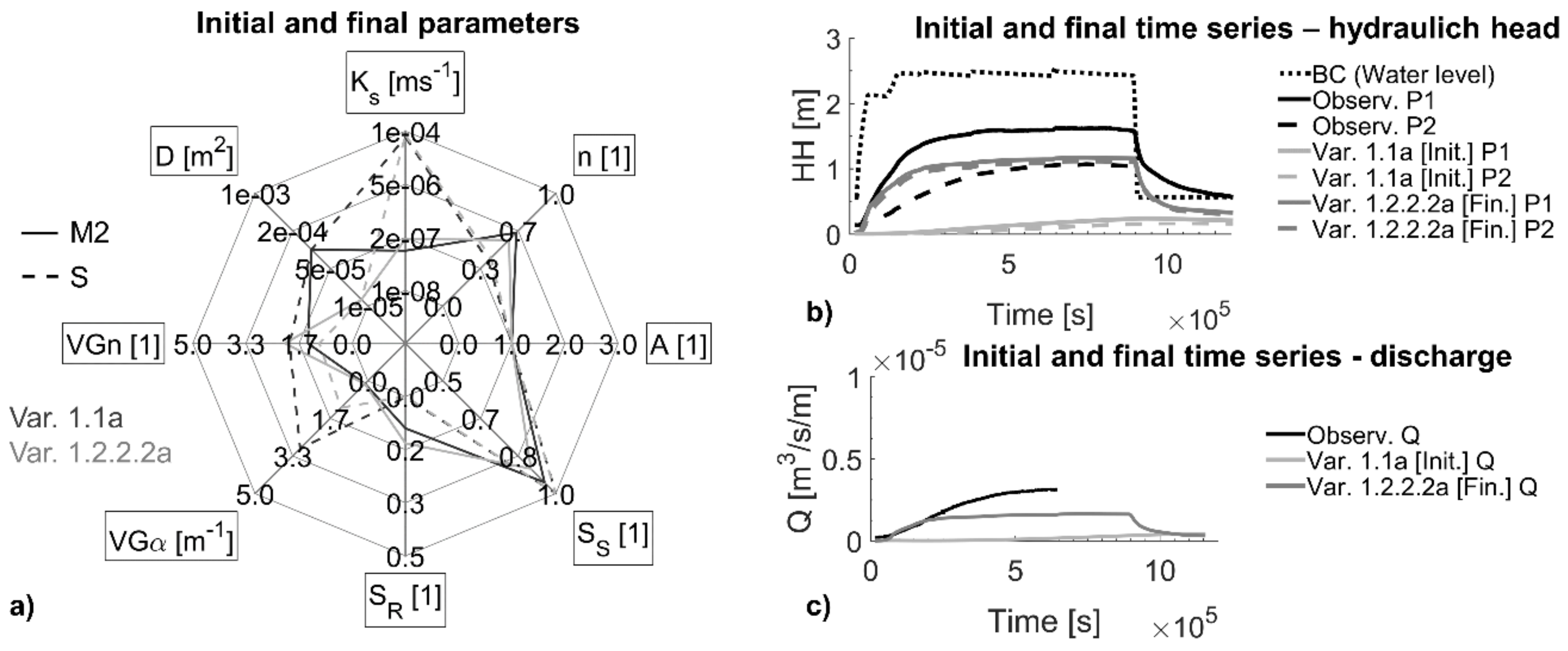
Both the initial input of Var 1.1a and the final estimations of Var. 1.2.2.2a are displayed in Figure 7 with their associated curve approximations.
Comparing the initial and final parameters, the drainage area was reduced from 1 × 10⁻⁴ m2 to 1 × 10⁻⁵ m2 and the hydraulic conductivity increased slightly using PEST (Figure 7a), leading to an increased phreatic line (Figure 7b dark line), while the hydraulic gradient remained low.
A second approach (index b) was carried out with changes to the initial inputs in order to avoid terminations in local minima. The nomenclature generally follows the system explained for index a. In this approach, the initial hydraulic conductivity of the cover layer M2 was adjusted to Ks = 5.78 × 10⁻⁵ ms−1 based on the assumption of an average high infiltration rate observed in the double ring infiltration tests (Figure 2). The drainage element property was set to D = 1 × 10⁻⁴ m2. In contrast to approach a, in which the simulated HH time series at the initial iteration was very low (e.g., in Figure 7b “Var. 1.1a”), the HH time series at the initial iteration of approach b was considerably higher, even above the observation data. In this approach, PEST approximates the observation data starting from the top.
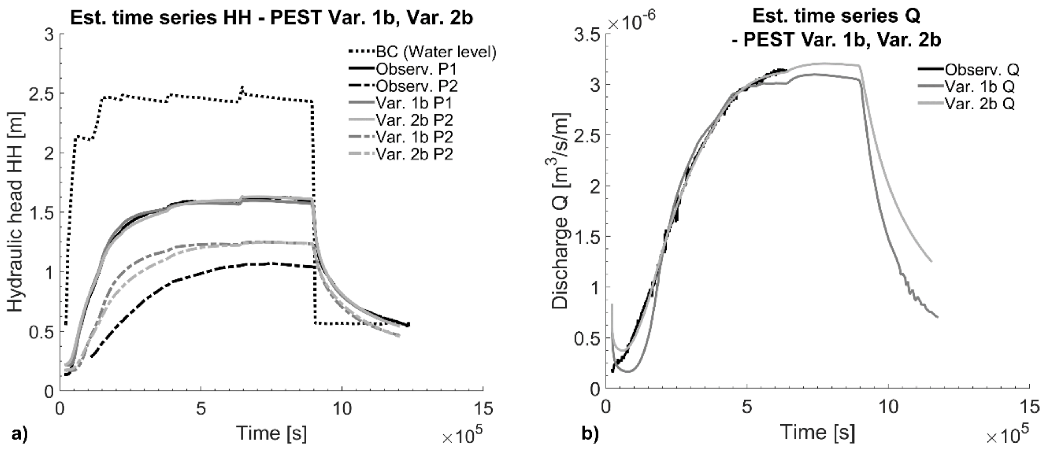
Approach b was also used to run Var. 2 and Var. 3 (Figure 5). The associated OBFs and their estimated parameters are compiled in Figure 8. Figure 9 contains the well-estimated time series for Var. 1b and Var. 2b (Var. 3b is not displayed as the fitting stopped early and resulted in an insufficient fitting with wSSRVar.3b = 479).
As shown in Figure 8a, the result of the OBF in Var. 1b decreased to wSSRVar. 1b = 20 (SSRVar.1b: 2.43; MSEVar. 1b= 0.085). The best fit, however, was found for Var. 2b, in which the minimum deviation was wSSRVar. 2b = 3 (SSR Var.2b = 1.64; MSE Var. 2b = 0.052). Figure 9 shows that larger model errors occur in piezometer P2, which are probably caused by the fixation of the drainage element property. It is known that better fitting results must exist for Var. 3b, e.g., by occupying the refined parameter zones of the cover layer with those parameters obtained by Var. 1b and Var. 2b, or that obtained by the AMALGAM approximation (compare Section 3.2).
With the PEST method, the anisotropy parameters in Var. 2b were estimated to A (PEST-Var. 2b, S) ≈ 0.55 and A (PEST-Var. 2b, M2) ≈ 0.16 (Figure 8b). The associated hydraulic conductivities of the cover layer (Ks(PEST-Var. 2b, M2, d1) = 1.39 × 10⁻⁶ ms−1; Ks(PEST-Var. 2b, M2, d2) = 3.94 × 10⁻⁶ ms−1) were therefore six times lower in the vertical than in the horizontal direction. When applying these anisotropy factors, the phreatic line in the dike body is slightly shifted downwards and leads to a more appropriate model fitting. However, the relevance of anisotropy factors in the present model is unclear, and an anisotropy of this magnitude in the sandy dike core is rather unlikely. For that reason, the PEST run for Var. 2b was repeated with fixed anisotropy AM2 = AS = 1 for the whole cross-section (Var. 2.1b). A second set of optimization runs was performed with adjusted initial inputs (obtained from Var. 2a) and an additional estimation on the drainage element property in order to reduce the residual deviation in piezometer P2 (Var. 2.2b). Compared to Var. 2b, both approaches did not improve the results (Figure 10).
3.2. Results from AMALGAM Optimization
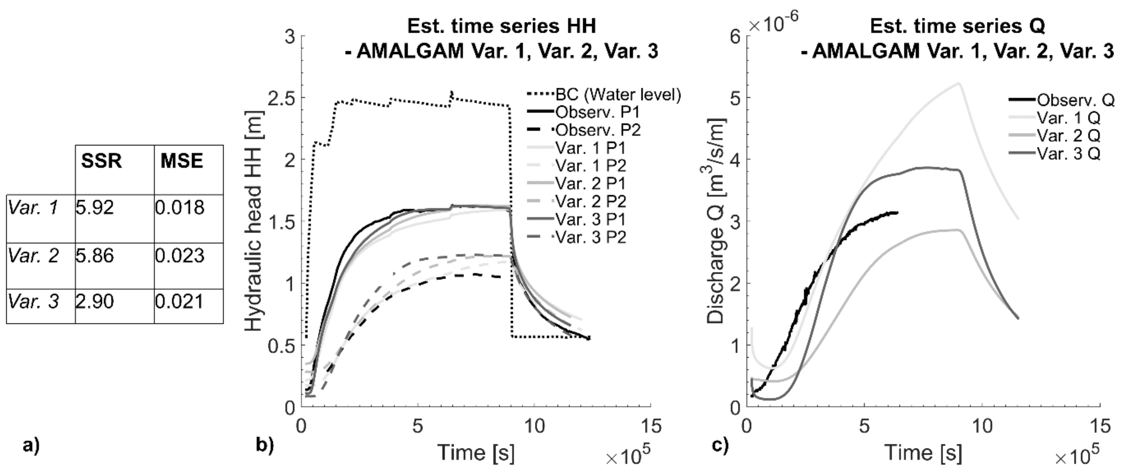
The results of the AMALGAM optimization for the three variations are shown in Figure 11 and Figure 12.
Regarding Figure 11, the HH time series in P1 are close to the measurement data in all three variations. Compared to these, higher residual deviations remain in piezometer P2, in which the water level exceeds the observation data by 0.2 m in all variations. For P2, the AMALGAM approximation does not provide significant improvements compared to Var. 1b and Var. 2b with PEST fitting (Figure 9). The computed discharge matches the observation data closely (MSEAMA-Var. 1, Q = 0.0018; MSEAMA-Var. 2, Q = 0.0025; MSEAMA-Var. 3, Q = 0.0014) but not perfectly with respect to the zero target. Moderate deviations are still present, e.g., in Var. 2 (after 6.3 × 10⁵ s), where the computed discharge is under-estimated by a factor of 0.84, or in Var. 1 where the computed discharge is over-estimated (factor 1.31).
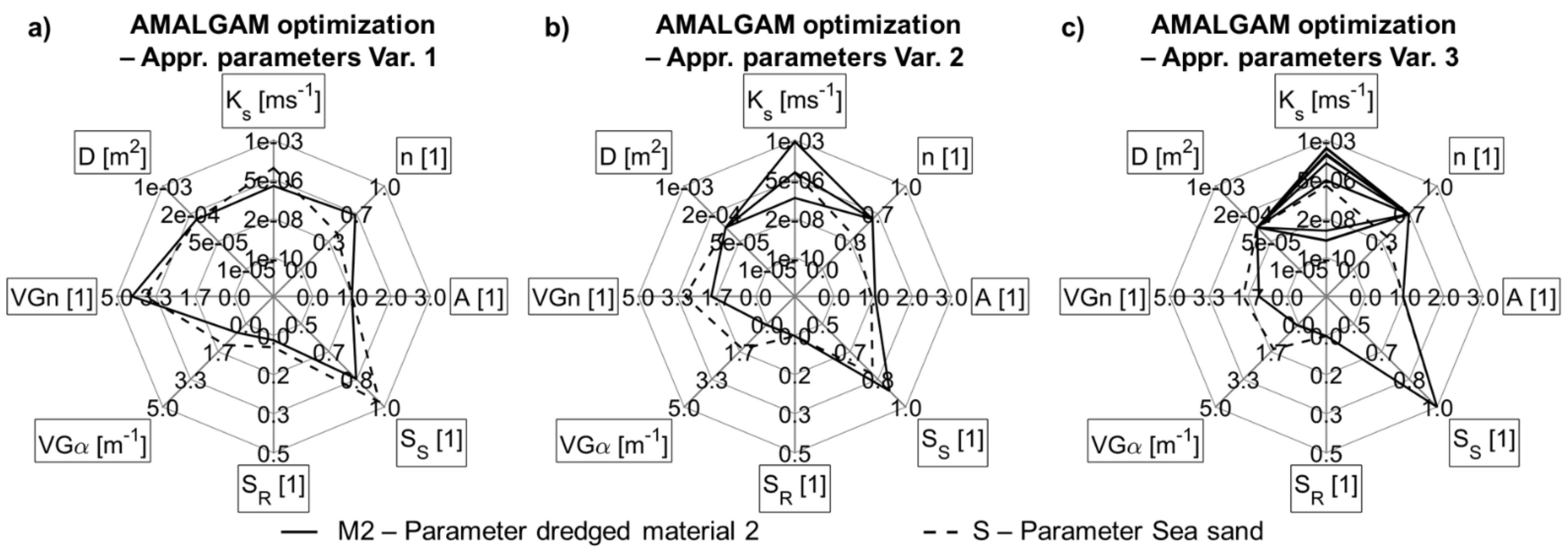
The corresponding parameters found by the AMALAGAM approximation are displayed in Figure 12. The AMALGAM results for Var. 1 (Figure 12a) indicate that the hydraulic conductivity of the cover layer (Ks(AMA-Var 1, M2) = 1.85 × 10⁻⁶ ms−1) may be lower than that of the sandy material in the dike core (Ks(AMA-Var. 1, S) = 2.19 × 10⁻⁵ ms−1), assuming that D = 1.55 × 10⁻⁴ m2 and an anisotropy coefficient of Α = 1 for the whole dike cross-section. Comparable results were obtained by the PEST fitting (Ks(PEST-Var. 1b, M2) 2.31 × 10⁻⁶ ms−1, Ks(PEST-Var. 1b, S) 1.73 × 10⁻⁵ ms−1), in which the anisotropy coefficients were found to be A(PEST-Var. 1b, S) = 0.31 and A(PEST-Var. 1b, M2) = 0.24 and the drainage area was fixed to D = 1 × 10⁻⁴ m−2 (Figure 7b, black lines).
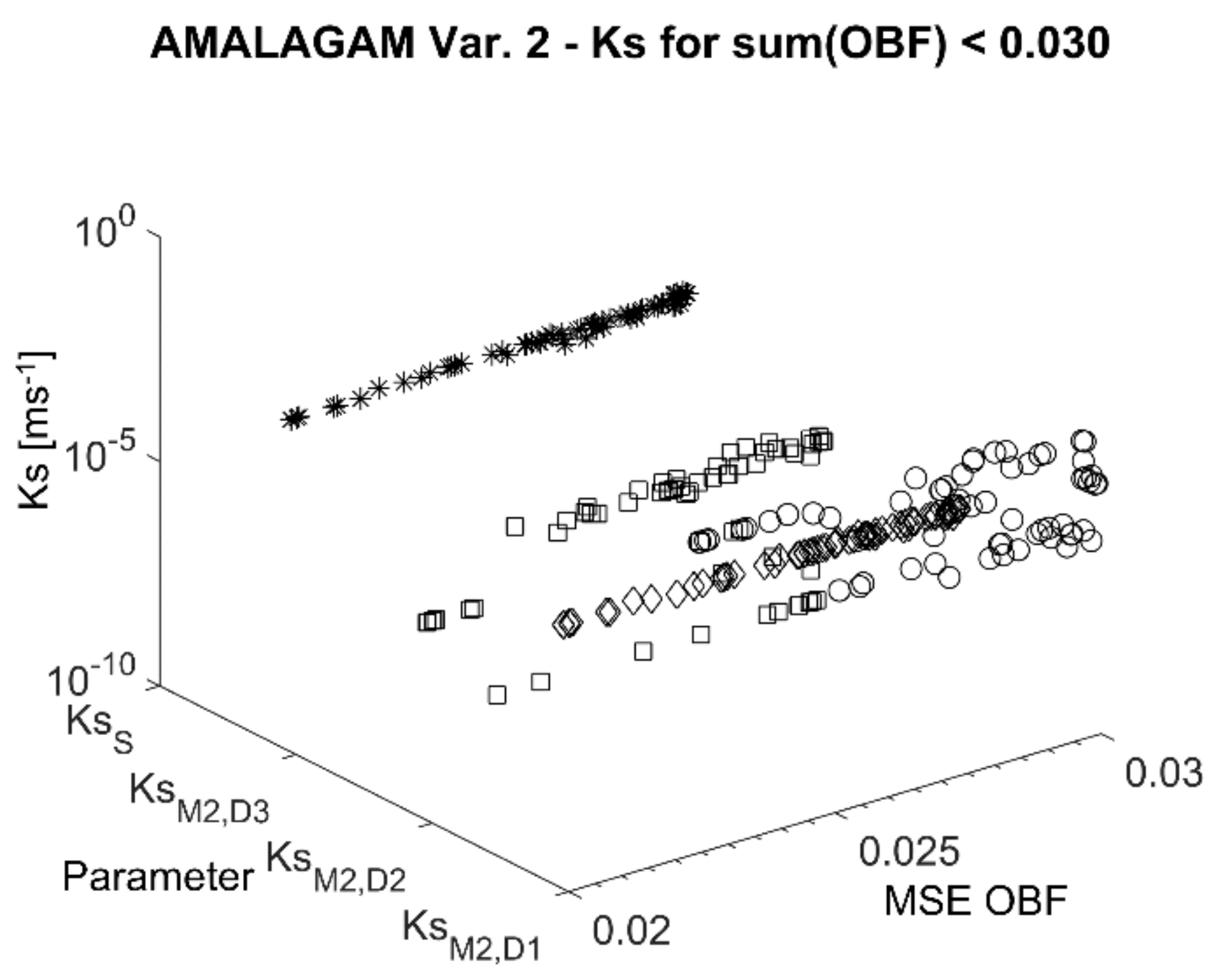
The AMALAGAM fitting applied to Var. 2 (Figure 11b) resulted in Ks values for M2 of Ks(AMA-Var. 2, M2, d1) = 1.33 × 10⁻⁵ ms−1 and Ks(AMA-Var2, M2, d2) = 3.59 × 10⁻⁸ ms−1 (Ks(AMA-Var2, M2, d3) = 1.15 × 10⁻⁸ ms−1). These values match the observation data obtained with both the double ring infiltration test (Ks(inf) ≈ 5.78 × 10⁻⁵ ms−1) and the laboratory analysis with undisturbed soil samples (Ks(Lab., undist.) < 6.02 × 10⁻⁸ ms−1) very closely. Compared to the PEST results (Ks(PEST-Var. 2b, M2, d1) = 1.39 × 10⁻⁶ ms−1; Ks(PEST-Var. 2b, M2, d2) = 3.98 × 10⁻⁶ ms−1 and Ks(PEST-Var. 2b, M2, d3) = 5.27 × 10⁻⁶ ms−1), AMALGAM predicts the Ks value in the deeper zone M2, d2 significantly lower by that in upper zone M2, d1. With both algorithms, minimum solutions could be derived either with comparably high Ks values in zone M2, d1 and low Ks values in zone M2, d2 (AMALGAM Var. 2), or with moderate Ks values for both zones (PEST Var. 2). Beyond that, AMALGAM found additional minima for different Ks parameter combinations within the Pareto front for similar model fittings in Var. 2 (Figure 13).
From Figure 13 it can be concluded that the Ks parameters vary within several orders of magnitude, while the model error remains small. Some of these combinations are comparable to the PEST results (Figure 8), however, the dependencies between these Ks values and the other parameters are not known.
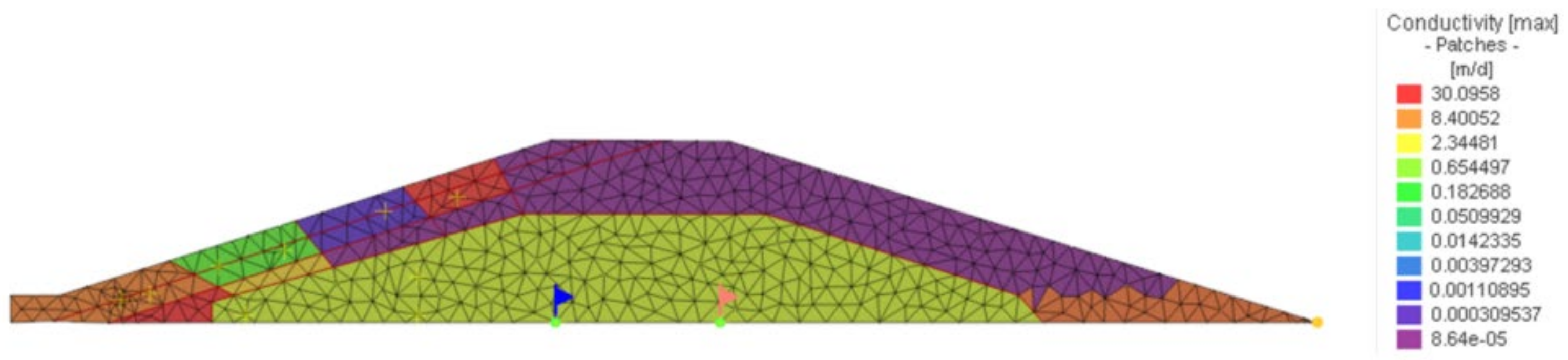
In contrast to the PEST approximation, acceptable estimations were found for Var. 3 using the AMALGAM algorithm. The Ks values of the cover layer sections vary from Ks,(AMA-Var. 3) = 1.0 × 10 −9 ms−1 (e.g., in zones M2, d2c, M2, d2d, and M2, d3a) up to Ks(AMA-Var. 3) = 3.48 × 10⁻⁴ ms−1 (in zones M2, d1d and M2, d2a) (Figure 12c, Figure 14), whereas the other parameters (e.g., Ks(AMA-Var. 3,S) = 1.81 × 10⁻⁵ ms−1, A = 1, D = 1 × 10⁻⁴ m2) do not differ significantly from Var. 2. In the model Var. 3, the dike cross-section primarily saturates from the dike toe upwards because the Ks values in these local zones are estimated to be equal to or even higher than those of the sandy dike core. In the upper sections of the cover layer, the model estimates very low Ks values for M2, d2c and M2, d2d; it thus predicts hardly any infiltration there. From the estimated parameters in model Var. 3, it can be concluded therefore that leakages occur primarily on the dike toe of the Rostock research dike, despite the knowledge that approaches with such constant parameter zones will not be the proper method to simulate preferential flow paths.
4. Discussion
4.1. Comparison of the Different Ks Values
The comparison of the characteristic soil parameters of the dredged material M2 from the laboratory analysis on disturbed samples (prepared in the automatic Proctor apparatus, Strassentest Type 770) with those determined with undisturbed samples and in field tests shows large differences in the Ks value—up to three orders of magnitude for the undisturbed samples and even more than three orders of magnitude for the field tests (Ks(Lab. undist., M2) < 6.02 × 10⁻⁸ ms−1, Ks(inf, M2) = 2.31 × 10⁻⁵–9.26 × 10⁻⁵ ms−1). With respect to the measured discharge in the quasi steady state (Q(at 9 × 10⁵ s) ≈ 3.13 × 10⁻⁶ m3s−1m−1) related to the infiltration area of the dike cross-section, the relative Ks value was determined to be Ks(rel, M2) = 4.98 × 10⁻⁷ ms−1. This may be considered as an effective material property of the cover layer as a whole. Therefore, in variation 1 of the numerical model, a homogenous cover layer was assumed.
The Ks values estimated with PEST and AMALGAM (Ks(PEST-Var. 1b, M2) = 2.31 × 10⁻⁶ ms−1; Ks(AMA-Var. 1, M2) = 1.85 × 10⁻⁶ ms−1) both match the Ks(rel, M2) closer than the Ks values from the laboratory and field analyses. Still, the estimated value Ks(AMA-Var. 1, M2) is four times higher than Ks(rel, M2), while the simulated discharge exceeds the measurement data only by a factor of 1.3 (Figure 11c).
4.2. Consideration of External Factors on Ks
It is known that the performance of the dike cover material can be strongly affected by external factors such as the climatic conditions, vegetation, and boring animals. The soil properties often change in seasonal fluctuation (e.g., by shrinking, swelling, or bioturbation) or because of aging effects (pedogenic processes). For grass rooted soils, Ks values of 3.0 × 10⁻⁵–4.0 × 10⁻³ ms−1 have been published in the literature [31], following a decreasing logarithmic function with the root depth for different types of vegetation [32]. The infiltration caused by leakages (e.g., desiccation cracks or animal boreholes) can be even higher [33], and it strongly depends on the individual structure of the leak (e.g., number, length, aperture, and connectivity) and the surrounding soil matrix [16]. In the case of small leaks, a general way to determine the effective hydraulic conductivity is by using average weighted “vertical” layers (Equation (4)) [34], which can be used to quantify the infiltration rate of grass layers [16]. Otherwise, the textured layer should be neglected [6]. In this context, only a few leaks with a connection into the sandy dike core have more relevance for the effective infiltration than a larger number of leaks ending inside a low-permeability layer [23].
where
- = weighted saturated hydraulic conductivity (ms−1)
- Ks(1) … Ks(n) = the saturated hydraulic conductivity of the vertical layer (ms−1)
- d1 … dn = the thickness of the vertical layer (m)
- d = the thickness of the total layer (m)
Using Equation (4) with Ks(rel, M2) as the average value (zone M2) and an average infiltration rate = Ks(M2, d1) = 5.79 × 10⁻⁵ ms−1 obtained by field measurement (Figure 2) in a textured/root-affected zone (d(M2, d1) = 0.85 m), the effective hydraulic conductivity for zone M2, d2 (d(M2, d2) = 0.30 m) is determined to be Ks(M2, d2) = 1.16 × 10⁻⁷ ms−1. The two-zone approach was studied in the model variation 2. With the AMALGAM algorithm, the estimated Ks values (Ks(AMA-Var 2, M2, d1) = 1.33 × 10⁻⁵ ms−1; Ks(AMA-Var 2, M2, d2) = 3.59 × 10⁻⁸ ms−1) are both lower than determined with Equation (4), and lead to a lower average value (Ks(M2) = 1.39 × 10⁻⁷ ms−1). Applying Equation (4) to the PEST results of Var. 2b the average Ks(M2) = 1.67 × 10⁻⁶ ms−1 is comparable with the AMALGAM result. However, the PEST results for the two-zone approach (Ks(PEST-Var. 2b, M2, d1) = 1.39 × 10⁻⁶ ms−1 < Ks(PEST-Var. 2b, M2, d2) = 3.94 × 10⁻⁶ ms−1) differ, and it is rather implausible that zone M2, d2 would be more permeable than zone M2, d1. Therefore, the parameters predicted by AMALGAM are more reliable for the physical interpretation of the two vertical cover layer zones.
4.3. Unexpected Results in Variation 3
The third variation is even more detailed. In this case, a simple method to determine an average Ks value is not available. Here, AMALGAM shows its full potential, leading to considerably more realistic results than PEST. However, there are also some issues that AMALGAM is not able to solve. In Var. 3, the cross-section primarily saturates through the dike toe. This may even be a realistic scenario—the cover material M2 was installed in layers on top of the profiled sand core [22]. In the toe region, a possible machine-induced deformation of the core cross-section together with the exact profile of the dike surface may have caused local areas with reduced cover layer thickness. More importantly, FDR probes were installed in the toe region after completion of the construction, for which holes were dug and refilled [13]. This may have caused imperfections or leaks resulting in higher infiltration rates. Although the AMALGAM result may be explained with possible realistic boundary conditions, this can only be seen as a strong hypothesis for the structure. The method seems to come to reasonable results, which can be used to look more closely into the real construction. In this particular example, the installation of instrumentation and possible resulting leaks may explain the observed differences in the phreatic line measurements of the two parallel dikes (east and west), of which only the eastern dike was modeled in detail in this study: phreatic lines inside the western dike core without installed probes at the dike toe raised up to a lower maximum of 0.5 m, with the same material properties and installation technology on both sides. This initial hypothesis was cross-checked using field infiltration tests and permeability analyses with undisturbed samples, indicating that high Ks values exist all over the dike surface and that the material is textured. These observations have been confirmed by suction pressure analysis [25], making again the approach of Var. 2 more realistic for the present problem.
4.4. Sensitivity of the Model Parameter VGS
Applying Equation (1) to calculate the sensitivities of the PEST iterations steps, they indicate a nonlinear behavior of the problem (Figure 15). Sensitivities with high variations are found for different iteration steps, and show varying sensitivities. Var. 1.1a for example shows moderate variations for almost all parameters, while for Var 1.2a the sensitives mostly remain low, except for VGSS(S) that becomes considerably high (same model, but different termination criteria). The sensitivity of VGSS(S) change with the implementation of the drainage element property (Var 1.2.2a; Var. 1.2.2.2a). In this case, the high sensitivity of VGSS(S) shifted to VGSR(S). In Var. 1.2.2.2a, the ratio between the sensitive parameters (VGSR(S) = 759; D = 696) and the insensitive parameters (Ks(M2) = 0.005; Ks(S) = 0.03; VGSS(M2) = 0.002) is more than 20,000, and is considered to be very high. In this case, it is recommended by Doherty [19,20] to fix up the insensitive parameters to encourage the PEST performance, which would mean that a fitting of the Ks values of the sea sand S in the dike core and the cover layer material M2 would not be possible in the current problem.
It was not expected that the fitting parameter VGSR(S) would partly become very sensitive. Due to the frequent flood simulation test performed at the facility, the measurement data generally refers to a dike body with a high initial saturation (S > 0.8; ψm > −15 kPa). The recorded initial moisture contents range from θ(M2) 0.48 to 0.53 (field moisture capacity ≈ 0.51–0.56), and quickly increase to the saturation value (θ(M2) 0.56–0.68).
The high initial saturation is also an explanation for a negligibly small hysteresis effect [25], because the initial unsaturated hydraulic conductivity is close to the saturated value. Assuming approaches of textured materials, the infiltration is concentrated in the macro pores, and the influence of matrix flow (both saturated and unsaturated) becomes low (insensitive matrix parameters).
4.5. Sensitivity of the Model Parameter VGα
The VGα fitting parameter is an indicator for the suction behavior of a soil. Empirical data of SWRC parameters for different soils can be found in the UNSODA database [35], using the RetC code [36], or by SWRC laboratory fitting. Using RetC, VGα = 0.5 m−1 (VGn = 1.09) indicates the suction behavior of a silty clay and VGα = 14.5 m−1 (VGn = 2.68) that of a sand. The AMALGAM optimization predicts VGα for M2 in a range of 0.078 m−1–0.52 m−1, and the PEST optimization VGα(M2) 0.09 m−1–0.57 m−1, both within a large constraint range of 0 m−1–5 m−1 chosen for the model approximation. In this context, the value VGα(M2) = 0.1 m−1 is seen as a very good fit because it matches the initial moisture content very closely. These results confirm the laboratory and field observations, and indicate that the dredged material M2 is characterized by very high suction potential.
For the sandy material in the dike core, VGα(S) values were determined with PEST ranging from 0.08 m−1 to 2.14 m−1, and with AMALGAM ranging from 1.26 m−1 to 1.51 m−1. These values were deliberately fixed in a parameter constraint range of 0.0 m−1 to 5.0 m−1 to account for the permanently recorded high water contents within the dike core (in the study, VGα(S) = 3.0 m−1 seems to be the most realistic value). However, assuming VGα(S) = 1.6 m−1 in the model indicates a suction behavior comparable to silty soils (RetC), and VGα(S) = 0.08 m−1 that of M2. In combination with the hydraulic conductivity of the sand, the saturation of the dike core is accelerated in the model, but there is no plausible physical interpretation for this result.
4.6. Comparison of Sensitivities
With respect to the high degree of initial saturation, a high sensitivity of the model parameter VGSR(S) had not been expected. At the permanent wilting point for sandy materials the volumetric water content is θR < 0.01 (RetC), and is often assumed to be equal to VGSR. In this context, a high sensitivity possibly occurred given the defined large constraint range (0–0.4) that was applied in the approximation. This may be an effect of the pedo-transfer function for the unsaturated conductivity. However, this does not explain the shift of the sensitivities for one, and the same unsaturated flow model. The most plausible explanation is that this is a result of model non-linearities. In comparison, the sensitivities of Ks are considerably low. This may be explained by an applied logarithmic parameter handle that was chosen in the PEST approximation in order to take account of the huge spread of the Ks parameter’s range. Hereinafter, the sensitives for the Ks-values are determined with a logarithmic function, and therefore they are not comparable to the other parameter in which the sensitivity is calculated with linear approaches. A similar sensitivity behavior was found by Hill [37]. In this study, the sensitivities evaluated for some of the initial parameter sets differ considerably from the sensitivities statistically obtained with other parameter sets.
4.7. Model Stability Testing
The model stability was checked using the JACTEST utility implemented in the PEST environment (see [19]). It was found out that numerical oscillations occur in the discharge computation if the value is close to zero. Assuming higher initial discharge rates in the model (ranging from 1.16 × 10⁻⁷ m3s−1m−1 to 5.79 × 10⁻⁷ m3s−1m−1) than observed by field measurement, the simulation becomes robust. However, this encourages the model error in the discharge value, because the simulated discharge decreases at the beginning of the simulation (e.g., in Figure 9 and Figure 11). With this setting, the infiltration should generally be accelerated. In the present model this is partly true; however, there is still a delay in the computed discharge time series compared to the measured data, which leads to the conclusion that there may be hydraulic bypasses along the dike base (e.g., caused by the wires of measurement probes) that dominate the hydraulic conductivity in the dike toe region and the sand core, comparable to the results of Var. 3b modeled with AMALGAM.
4.8. Eigenvalue Ratio and Condition Number
In general, the inverse modeling becomes a hard challenge if the considered problem is strongly ill-posed [19]. Hereinafter, the ratio of largest/lowest Eigenvalue and the condition number are indicators for the suitability of the PEST fitting. If the Eigenvalue ratio exceeds 107 or the condition number exceeds 104, PEST cannot calculate the parameter upgrade vector appropriately, due to the insensitivity of a (group of) parameter(s) or the correlation [19]. According to the PEST record files obtained in the present study, the determined ratios of highest/lowest eigenvalue are as follows: Var. 1b = 4 × 10⁸; Var. 2b = 5 × 10¹⁰; Var. 3b = 5 × 10¹⁰. All three eigenvalue ratios are higher than 107, indicating an ill-posedness. The critical condition number is exceeded in Var. 1b for 0% of the iterations, in Var. 2b for 16.7% of the iterations and in Var. 3b for 93.3% of the iterations. Especially the condition numbers in Var. 3b indicate a high non-uniqueness of the parameters. This confirms an increasing model complexity and explains why in the PEST approximations no reliable fitting result could be obtained for Var. 3a/b.
5. Conclusions
In the DredgDikes project, a large amount of observation data was obtained in several field experiments on the Rostock research dike, which has been built from dredged materials from the German Baltic Sea area. The field observations indicate considerable differences in hydraulic material behavior compared to that obtained by laboratory testing. Since it is necessary to quantify the effective properties of the materials used as replacement materials for other dike cover materials, two inverse modeling techniques (PEST, AMALGAM) were applied to gain insight into the hydraulic mechanisms inside the dredged material. At the same time, the methods were evaluated regarding their effectiveness and accuracy in modeling the system, with a focus on realistic physical explanations compared to the field measurements.
The proposed inverse techniques are useful in the model fitting. However, some sophisticated model fittings were found with Feflow, and residual deviations between the simulated and observed data are still present (e.g., in the discharge simulation). It is generally known that a numerical computation of the water movement in soils involves many uncertainties (numerical uncertainties, measurement uncertainties, uncertainties by the model setup, etc.). The accuracy of the proposed model results therefore needs to be considered carefully. The results are strongly dependent on the chosen numerical solver, the water movement equation, the model setup and the applied search algorithm. Applying another numerical solver may provide different results.
The following main conclusions can be drawn:
- PEST and AMALGAM are both powerful tools for parameter estimation. For the studied problem of dike infiltration on the Rostock research dike facility, PEST showed a number of shortcomings. The quality of the PEST fitting strongly depends on the initial input, the initial conditions and the termination criteria. In addition, the PEST algorithm frequently hangs up in local minima. It is unclear how close these results match the global optimum. Compared with the AMALGAM optimization it can be seen that the more complex the system gets, the more likely it is that PEST finds local minima that are quite far from an optimum solution;
- Multi-objective minimization and Pareto analysis methods are useful for the present problem, as shown in Figure 12. Due to multi-objective approach, AMALAGAM is less susceptible for local minima termination, and is robust against weak initial inputs and weighting strategies. However, the algorithm is comparably time-consuming, and a proper interpretation of the Pareto results is difficult without knowledge about the exact parameter dependencies;
- The natural process of dike infiltration is a complex non-linear process and is coupled with multiple parameter dependencies. Such non-linear dependencies are difficult to rate and analyze by conventional multivariate methods (e.g., main component analysis) without additional pre-knowledge information. However, these dependencies are important for the quantification of the effectivity of the material properties, and help to understand the non-linear model behavior;
- The estimation of hydraulic soil properties for fine-grained dredged materials with high organic contents used as cover material in dike construction is difficult. Based on the modeling results (Ks(PEST-Var 1, M2); Ks(PEST-Var 2, M2, d1); Ks(PEST-Var 2, M2, de); Ks(AMA-Var 1, M2)), it may be concluded that the effective hydraulic conductivity Ks of the material M2 ranges approximately from 1.39 × 10⁻⁶ ms−1 to 3.94 × 10⁻⁶ ms−1;
- The Ks values obtained from laboratory analysis with undisturbed soil samples differ from the realistic behavior by approximately two orders of magnitude. In practice, undisturbed samples would have to be taken from a testing field under field compaction conditions, which would have to be installed during the planning phase usually long before contracting the dike construction;
- Ks values obtained from laboratory analysis with disturbed soil samples are usually easy to obtain; however, the difference from realistic field values accounts for even more than three orders of magnitude, particularly if the samples are prepared with optimal density in the Proctor apparatus;
- The scenario resulting in the most realistic results for the present study is to simulate the dike infiltration with the two-zone approach using Variant 2, in which the upper zone M2, d1 is structured, and therefore more permeable (Ks(AMA-Var.2,M2, d1) = 1.33 × 10⁻⁵ ms−1) than the deeper zone M2, d2 (Ks(AMA-Var2, M2, d2) = 3.59 × 10⁻⁸ ms−1);
- Field infiltration test data are useful to quantify the infiltration rate for the upper zone of the dike cover layer, made of dredged material with high organic content. To quantify the Ks value of the lower zone, additional field testing would be needed, or, alternatively, laboratory test data can be used considering the computed deviations. The application of upper zone field infiltration data for the whole thickness of the dike cover would result in unrealistically high Ks values. Still, infiltration tests can only be performed on existing dikes (or testing fields, see above);
- In the present case, the estimation of an averaged Ks value determined in the laboratory from disturbed soil samples, and with an offset of three orders of magnitude applied, seems to be a suitable method for dike design;
- Another powerful family of multivariate analysis methods are artificial neuronal networks (ANN), which may help to identify the non-linear parameter dependencies of the materials’ hydraulic properties [38]. In this context, the application of an ANN surrogate model may be a reasonable approach to analyzing the relationship between multiple parameters and to explore further minima, as was already successfully applied to Feflow simulations by Arndt et al. [39]. This is an issue of the current research activities of the first author, and will be published in the near future.
Author Contributions
Conceptualization, T.J. and S.C.; methodology, T.J.; software, T.J.; validation, T.J. and S.C.; formal analysis, T.J.; investigation, T.J., S.C. and F.S.; resources, S.C. and F.S.; data curation, T.J.; writing—original draft preparation, T.J.; writing—review and editing, S.C.; visualization, T.J.; supervision, F.S.; project administration, S.C. and F.S.; funding acquisition, S.C. and F.S. All authors have read and agreed to the published version of the manuscript.
Funding
The field and laboratory data was derived in the EU cooperation project DredgDikes, funded by the Interreg IV South Baltic Programme. We acknowledge financial support by Deutsche Forschungsgemeinschaft and Universität Rostock within the funding programme Open Access Publishing.
Institutional Review Board Statement
Not applicable.
Informed Consent Statement
Not applicable.
Data Availability Statement
The data presented in this study are available on request from the corresponding author.
Conflicts of Interest
The authors declare no conflict of interest.
Abbreviations
| AMALGAM | A multi-algorithm, genetically adaptive multi-objective algorithm |
| BC | Boundary condition for model |
| FePEST | PEST algorithm implemented in FEFLOW |
| GCL | Geosynthetic clay liner |
| M2 | Cover layer material for cover layer on the Rostock research dike called “M2” |
| MSE | Mean square error |
| OBF | objective function |
| P1, P2 | Piezometer pipe for hydraulic head observation |
| PEST | Parameter estimation tool |
| S | Sea sand |
| SSR | Sum of square residual |
| TOC | Total organic content |
| wSSR | Weighted sum of square residual |
| Variables | |
| A | Anisotropy factor for hydraulic conductivity (1) |
| d | Layer thickness of the dike cover layer and local zones (m) |
| D | Drainage element parameter respecting a drainage composite in the model (m²) |
| HH | Hydraulic head (m) |
| Ks | Saturated hydraulic conductivity (ms−1) |
| Average layer weighted hydraulic conductivity (ms−1) | |
| n | Pore void ratio of the porous media (1) |
| Q | Discharge of drainage water (m3s−1m−1) |
| VGα | VanGenuchten curve fitting parameter (m−1) |
| VGn | VanGenuchten curve fitting parameters (1) |
| VGSR | VanGenuchten fitting parameter for residual saturation (1) |
| VGSS | VanGenuchten fitting parameter for maximal saturation (1) |
| Ψ | Permittivity (ls−1) |
| ψm | Matric potential equal to suction pressure (kPa) |
| φ | Objective function (OBF) |
| θ | Volumetric water content (1) |
| Indices | |
| a | Index notation for PEST fitting using laboratory as initial input |
| AMA | Index notation for AMALGAM approximation |
| b | Index notation for PEST fitting using infiltration test data as initial input |
| Lab. dist. | Index notation for disturbed soil sample analysis in laboratory (Ks(Lab. dist.)) |
| Lab. undist. | Index notation for undisturbed soil sample in laboratory (Ks(Lab. undist.)) |
| M2 | Index notation for the total zone of the dike cover layer |
| M2d1, M2d2, M2d3… | Index notation for local model zones of the dike cover layer |
| PEST | Index notation for PEST approximation |
| rel. | Index notation for relative saturated conductivity calculated by discharge data (Ks(rel.)) |
| S | index notation for the total zone of the dike core (made by the Sea sand “S”) |
| Var. (item) | Index notation for different model variants (according to Figure 5) and repetitions (sub item) under |
References
- EAK. Empfehlungen für die Ausführung von Küstenschutzwerken: (Korrigierte Ausgabe 2007); Westholsteinische Verl.-Anst. Boyens: Heide, Germany, 2002; ISBN 978-3-8042-1056-1. (in German) [Google Scholar]
- CIRIA. The International Levee Handbook; CIRIA: London, UK, 2013; ISBN 9780860177319. [Google Scholar]
- DIN 19172. German Standard. Hochwasserschutzanlagen an Fließgewässern [Flood Protection Works on Rivers]; Beuth: Berlin, Germany, 2013. (in German) [Google Scholar] [CrossRef]
- DWA-M 507-1. Merkblatt DWA-M 507-1: Deiche an Fließgewässern; Teil 1: Planung, Bau und Betrieb; Deutsche Vereinigung für Wasserwirtschaft Abwasser und Abfall: Hennef, Germany, 2011. (in German) [Google Scholar]
- EN 1997. Eurocode 7 Geotechnical Design; European Committee for Standardization: Brussels, Belgium, 1997. [Google Scholar]
- Temmler, H. Sickervorgänge in Deichen und ihre Auswirkung auf die Sturmflutsicherheit; Fachausschuss für Küstenschutzwerke Workshop: Aus der Arbeit des Fachausschuss Küstenschutzwerke Strategien, Sicherheit und Bemessung (Sprechtag: Laufende Arbeiten und künftige Projekte); HTG und DGGT: Hamburg, Germany, 2009. (in German) [Google Scholar]
- Heyer, D.; Schmutterer, C. Dichtungssysteme in Deichen. In Wasserbaukolloqium 2005, Stauanlagen am Beginn des 21. Jahrhunderts; TU Dresden Fakultät Bauingenieurwesen—Institut für Wasserbau und Technische Hydromechanik: Dresden, Germany, 2005. (in German) [Google Scholar]
- Saathoff, F.; Cantré, S.; Sikora, Z. South Baltic Guidline for the Application of Dredged Materials, Coal Combustion Products and Geosynthetics in Dike Construction: [Project] DredgDikes; Univ. Agrar- und Umweltwiss. Fakultät: Rostock, Germany, 2015; ISBN 978-3-86009-423-5. [Google Scholar]
- HTG. Fachbericht Verwertung von Feinkörnigem Baggergut im Bereich der Deutschen Küste [Beneficial Recovery of Fine-Graines Dredged Material at the German Coast]; Hafentechnische Gesellschaft: Hamburg, Germany, 2006. (in German) [Google Scholar]
- Gebert, J.; Groengroeft, A. Long-term hydraulic behaviour and soil ripening processes in a dike constructed from dredged material. J. Soils Sediments 2020, 20, 1793–1805. [Google Scholar] [CrossRef] [Green Version]
- Oing, K.; Gröngröft, A.; Eschenbach, A. Ripening reduces the shrinkage of processed dredged material. J. Soils Sediments 2020, 20, 571–583. [Google Scholar] [CrossRef]
- PIANC. Dredged Materials as a Resource: Options and Constraints, PIANC Report no. 104 EnviCom Working Group 104. 2009. Available online: www.pianc.org (accessed on 20 August 2020).
- Nitschke, E.; Cantré, S.; Saathoff, F. Full-Scale Seepage Experiments at the German DredgDikes Research Dike. In Proceedings of the South Baltic Conference on Dredged Materials in Dike Construction, Rostock, Germany, 10–12 April 2014; University of Rostock: Rostock, Germany, 2014; pp. 53–59. [Google Scholar] [CrossRef]
- Diersch, H.-J.G. FEFLOW: Finite Element Modeling of Flow, Mass and Heat Transport in Porous and Fractured Media; Springer: Berlin/Heidelberg, Germany, 2014. [Google Scholar] [CrossRef]
- Sleep, M.D. Analysis of Transient Seepage Through Levees. Ph.D. Thesis, Virginia Polytechnic Institute and State University Blacksburgh, Blacksburgh, VA, USA, 2011. [Google Scholar]
- Haselsteiner, R. Deiche an Fließgewässern und ihre Durchsickerung. Ph.D Thesis, TU München, München, Germany, 2007. (in German). [Google Scholar]
- Yeh, W.W.G. Review of Parameter Identification Procedures in Groundwater Hydrology: The Inverse Problem. Water Resour. Res. 1986, 22, 95–108. [Google Scholar] [CrossRef]
- Doherty, J. PEST—The Book: Calibration and Uncertainty Analysis for Complex Environmental Models; Watermark Numerical Computation: Brisbane, Australia, 2015; 227p, ISBN 978-0-9943786-0-6. [Google Scholar]
- Doherty, J. PEST, Model-Independent Parameter Estimation; User Manual Part 1: PEST, SENSAN, and Global Optimisers; Watermark Numerical Computing: Brisbane, Australia, 2019. [Google Scholar]
- Doherty, J. PEST, Model-Independent Parameter Estimation; User Manual Part 2: PEST Utility Support Software; Watermark Numerical Computing: Brisbane, Australia, 2019. [Google Scholar]
- Vrugt, J.A. Multi-Criteria Optimization Using the AMALGAM Software Package: Theory, Concepts, and MATLAB Implementation; University of California Irvine: Irvine, CA, USA, 2016. [Google Scholar]
- Cantré, S.; Saathoff, F. Installation of fine-grained organic dredged materials in combination with geosynthetics in the German DredgDikes research dike facility. Eng. Struc. Tech. 2013, 5, 93–102. [Google Scholar] [CrossRef]
- Khandelwal, S. Effect of Desiccation Cracks on Earth Embankments. Master‘s Thesis, Texas A & M University, Galveston, TX, USA, 2011. [Google Scholar]
- Šimůnek, J.; Jarvis, N.J.; Van Genuchten, M.; Gärdenäs, A. Review and comparison of models for describing non-equilibrium and preferential flow and transport in the vadose zone. J. Hydrol. 2003, 272, 14–35. [Google Scholar] [CrossRef]
- Jurisch, T.; Cantré, S.; Saathoff, F. Infiltration behaviour of dike covers made of dredged material on the Rostock Research dike. E3S Web Conf. 2020, 195, 01032. [Google Scholar] [CrossRef]
- Van Genuchten, M.T. A Closed-form Equation for Predicting the Hydraulic Conductivity of Unsaturated Soils. Soil Sci. Soc. Am. J. 1980, 44, 892–898. [Google Scholar] [CrossRef] [Green Version]
- DIN 19682-7. German Standard. Soil Quality-Field Tests-Part 7: Determination of Infiltration Rate by Double Ring Infiltrometer; Beuth: Berlin, Germany, 2015; (in German). [Google Scholar] [CrossRef]
- DIN 18130-1. German Standard. Soil - Investigation and Testing; Determination of the Coefficient of Water Permeability - Part 1: Laboratory Tests; Beuth: Berlin, Germany, 1998. (in German) [Google Scholar]
- Mike. FePEST in FEFLOW 7.0- User Guide. 2015. Available online: www.mikepoweredbydhi.com (accessed on 10 September 2020).
- Efstratiadis, A.; Koutsoyiannis, D. One decade of multi-objective calibration approaches in hydrological modelling: A review. Hydrol. Sci. J. 2010, 55, 58–78. [Google Scholar] [CrossRef] [Green Version]
- Roy, J.W.; Parkin, G.W.; Wagner-Riddle, C. Water Flow in Unsaturated Soil Below Turfgrass Observations and LEACHM (within EXPRES) Predictions. Soil Sci. Soc. Am. J. 2000, 64, 86–93. [Google Scholar] [CrossRef]
- Husicka, A. Vegetation, Ökologie und Erosionsfestigkeiten von Grasnarben auf Flussdeichen am Beispiel der Rheindeiche in Nordrhein-Westfahlen; Dissertationes Botanicae, Band 379. Verlag J. Cramer; Gebrüder Borntraeger Verlagbuchhandlung: Berlin, Germany, 2003. (in German) [Google Scholar]
- Brauns, J. Wasserverluste und Durchsickerung von Leckagen in schmalen Dammdichtungen. Wasserwirtschaft 1978, 69, 351–356. (in German). [Google Scholar]
- Goris, A.; Schneider, K.-J. Bautabellen für Ingenieure, mit Berechnungshinweisen und Beispielen; Werner Verlag, Wollters Kluwer: Köln, Germany, 2010. [Google Scholar]
- Tuller, M.; Or, D. Water retention and characteristic curve. In Encyclopedia of Soils in the Environment; Elsevier: Hoboken, NJ, USA, 2004; pp. 278–289. [Google Scholar]
- Van Genuchten, M.V.; Leij, F.J.; Yates, S.R. The RETC Code for Quantifying Hydraulic Functions of Unsaturated Soils; Robert S. Kerr Environmental Research Laboratory: Ada, OK, USA, 1991. [Google Scholar]
- Hill, M.C. Methods and Guidelines for Effective Model Calibration. Build. Partnersh. 2000, 1–10. [Google Scholar] [CrossRef] [Green Version]
- Zhang, G.; Patuwo, B.E.; Hu, M.Y. Forecasting with artificial neural networks. Int. J. Forecast. 1998, 14, 35–62. [Google Scholar] [CrossRef]
- Arndt, O.; Barth, T.; Freisleben, B.; Grauer, M. Approximating a finite element model by neural network prediction for facility optimization in groundwater engineering. Eur. J. Oper. Res. 2005, 166, 769–781. [Google Scholar] [CrossRef]
Figure 1.
Cross-section D (east) of Rostock research dike.

Figure 2.
Results of double ring infiltration test on the eastern slope of cross-section D of Rostock research dike.
Figure 2.
Results of double ring infiltration test on the eastern slope of cross-section D of Rostock research dike.

Figure 3.
Soil profile analysis after infiltration test: (a) location VI (centre, left); (b) location IV (top, left) with small vertical crack structure and moderate infiltration; (c) location III (centre, left) with highest infiltration and strong soil texture; (d) location Va (top, right) with low infiltration and no desiccation cracks.

Figure 4.
Observation data for the model fitting on cross-section D, recorded hydraulic head HH and discharge Q [13].
Figure 4.
Observation data for the model fitting on cross-section D, recorded hydraulic head HH and discharge Q [13].

Figure 5.
Applied model variations with model sections of the cover layer and respective parameters.
Figure 5.
Applied model variations with model sections of the cover layer and respective parameters.

Figure 6.
Objective functions (OBF) of PEST optimization for Var. 1a with different adjustments in the initial parameters, the termination criteria and parameter combinations.
Figure 6.
Objective functions (OBF) of PEST optimization for Var. 1a with different adjustments in the initial parameters, the termination criteria and parameter combinations.

Figure 7.
(a) Initial (laboratory) parameters used in Var 1.1a, “black” and final parameters estimated in Var. 1.2.2.2a, “grey”; (b,c) corresponding time series for initial and final approximation.
Figure 7.
(a) Initial (laboratory) parameters used in Var 1.1a, “black” and final parameters estimated in Var. 1.2.2.2a, “grey”; (b,c) corresponding time series for initial and final approximation.

Figure 8.
(a) PEST OBF minimization for Var. 1b–3b; (b) estimated parameters for Var. 1b–3b.

Figure 9.
(a) PEST approximation of the hydraulic head time series for Var. 1b and 2b; (b) PEST approximation of the discharge time series for Var. 1b and 2b.
Figure 9.
(a) PEST approximation of the hydraulic head time series for Var. 1b and 2b; (b) PEST approximation of the discharge time series for Var. 1b and 2b.

Figure 10.
(a) PEST OBF for Var. 2.1b and Var. 2.2b; (b) estimated parameters for Var. 2.1b and Var. 2.2b.
Figure 10.
(a) PEST OBF for Var. 2.1b and Var. 2.2b; (b) estimated parameters for Var. 2.1b and Var. 2.2b.

Figure 11.
(a) Model error; (b) time series of AMALGAM approximation on hydraulic head data; (c) time series of AMALGAM approximation on discharge.
Figure 11.
(a) Model error; (b) time series of AMALGAM approximation on hydraulic head data; (c) time series of AMALGAM approximation on discharge.

Figure 12.
Estimated parameters of the AMALGAM approximation for (a) Var. 1, (b) Var. 2 and (c) Var. 3.
Figure 12.
Estimated parameters of the AMALGAM approximation for (a) Var. 1, (b) Var. 2 and (c) Var. 3.

Figure 13.
Pareto combinations of the Ks value obtained by the AMALGAM approximation for Var. 2.

Figure 14.
Saturated hydraulic conductivity in Var. 3 estimated with AMALAGAM.

Figure 15.
Sensitives per iteration step for selected PEST optimization.


Table 1.
Properties of dredged material M2 and sea sand S [8].
Table 1.
Properties of dredged material M2 and sea sand S [8].
| Property | Standard | Unit | M2 | S |
|---|---|---|---|---|
| TOC | ISO 10694 | (%) | 5–6 | 0 |
| Ks(Lab,dist.) | DIN 18128 | (ms−1) | 5 × 10⁻¹⁰ … 4 × 10⁻⁹ | 8.5 × 10⁻⁵ |
| Ks(Lab,undist.) | DIN 18128 | (ms−1) | 4 × 10⁻⁸ … 6 × 10⁻⁸ | - |
| Pore void n | - | (1) | 0.59 … 0.66 | 0.4 |
| Grain sizes | ISO 11277 | (%) | 45/33/22 | 98 / 2 / 0 |
| (s/si/cl) | ||||
| Density | - | (gcm−3) | 1.48 … 1.54 | 1.8 |
| Dry density | - | (gcm−3) | 0.87 … 1.09 | 1.6 |
Publisher’s Note: MDPI stays neutral with regard to jurisdictional claims in published maps and institutional affiliations. |
© 2021 by the authors. Licensee MDPI, Basel, Switzerland. This article is an open access article distributed under the terms and conditions of the Creative Commons Attribution (CC BY) license (http://creativecommons.org/licenses/by/4.0/).
Share and Cite
MDPI and ACS Style
Jurisch, T.; Cantré, S.; Saathoff, F. Inverse Infiltration Modeling of Dike Covers Made of Dredged Material Using PEST and AMALGAM. Geosciences 2021, 11, 41. https://doi.org/10.3390/geosciences11020041
AMA Style
Jurisch T, Cantré S, Saathoff F. Inverse Infiltration Modeling of Dike Covers Made of Dredged Material Using PEST and AMALGAM. Geosciences. 2021; 11(2):41. https://doi.org/10.3390/geosciences11020041
Chicago/Turabian StyleJurisch, Tim, Stefan Cantré, and Fokke Saathoff. 2021. "Inverse Infiltration Modeling of Dike Covers Made of Dredged Material Using PEST and AMALGAM" Geosciences 11, no. 2: 41. https://doi.org/10.3390/geosciences11020041
Note that from the first issue of 2016, this journal uses article numbers instead of page numbers. See further details here.