Article

Internal Friction Angle of Cohesionless Binary Mixture Sand–Granular Rubber Using Experimental Study and Machine Learning †

by
Firas Daghistani
1,2,
Abolfazl Baghbani
3,
Hossam Abuel Naga
1,* and
Roohollah Shirani Faradonbeh
4
1
Department of Civil Engineering, La Trobe University, Bundoora, VIC 3086, Australia
2
Civil Engineering Department, University of Business and Technology, Jeddah 21448, Saudi Arabia
3
School of Engineering, Deakin University, Geelong, VIC 3216, Australia
4
WA School of Mines, Minerals, Energy and Chemical Engineering, Curtin University, Kalgoorlie, WA 6430, Australia
*
Author to whom correspondence should be addressed.
This paper is part of the PhD of the first author.
Geosciences 2023, 13(7), 197; https://doi.org/10.3390/geosciences13070197
Submission received: 31 March 2023 / Revised: 17 May 2023 / Accepted: 25 June 2023 / Published: 28 June 2023
(This article belongs to the Collection New Advances in Geotechnical Engineering)

Abstract

:
This study aimed to examine the shear strength characteristics of sand–granular rubber mixtures in direct shear tests. Two different sizes of rubber and one of sand were used in the experiment, with the sand being mixed with various percentages of rubber (0%, 10%, 20%, 30%, and 50%). The mixtures were prepared at three different densities (loose, slightly dense, and dense), and shear stress was tested at four normal stresses (30, 55, 105, and 200 kPa). The results of 80 direct shear tests were used to calculate the peak and residual internal friction angles of the mixtures, and it was found that the normal stress had a significant effect on the internal friction angle, with an increase in normal stress leading to a decrease in the internal friction angle. These results indicated that the Mohr–Coulomb theory, which applies to rigid particles only, is not applicable in sand–rubber mixtures, where stiff particles (sand) and soft particles (rubber) are mixed. The shear strength of the mixtures was also influenced by multiple factors, including particle morphology (size ratio, shape, and gradation), mixture density, and normal stress. For the first time in the literature, genetic programming, classification and regression random forests, and multiple linear regression were used to predict the peak and residual internal friction angles. The genetic programming resulted in the creation of two new equations based on mixture unit weight, normal stress, and rubber content. Both artificial intelligence models were found to be capable of accurately predicting the peak and residual internal friction angles of sand–rubber mixtures.

1. Introduction

According to recent estimates, the number of discarded tires worldwide is approximately 1.5 billion per year. This trend has shown an upward trajectory over time and is projected to continue its growth into the future [1,2,3]. An analysis of waste tire data from the year 2009–2010 in Australia reveals that there were approximately 48 million equivalent passenger units (EPU) of waste tires. Out of these, 66% were either disposed of in landfills or illegally stockpiled, 16% were recycled domestically, and 18% were exported [4]. The non-biodegradable nature of waste tires, coupled with their accumulation in stockpiles, has resulted in not only unpleasant visual impacts but also environmental pollution and hazards due to their flammability [5]. The occurrence of a tire fire releases toxic smoke into the atmosphere, negatively impacting air quality and visibility in the surrounding area [6,7].
It is possible to reduce the global tire waste disposal problem by using recycled waste tire rubbers in engineering applications [8]. Rubber tires have many properties that make them suitable for use in engineering applications, such as their high durability, their high permeability, and their low bulk density [9,10,11,12,13]. These properties make tire waste an excellent material for geotechnical engineering and construction applications, such as lightweight fillers [14,15,16,17,18], highway construction [16,17,18,19,20,21], soil reinforcement [22,23], soil retention walls [24,25], slope stabilization [18,26], aggregates in landfill leach beds [27], additive to asphalt [21,27], freezing depth limiter [28], vibration isolation [29], and for low-strength but ductile concrete [30].
According to the American Society of Testing and Materials [31,32], a variety of sizes can be produced by processing rubber tires, including shreds, chips, granular, ground, and powder. Tire shreds are scrap pieces of tires that are shaped like basic geometric forms. They vary in size from 50 to 305 mm. Tire chips are like tire shreds, but most of the wire has been removed and they are smaller, ranging from 12 to 50 mm. Granulated rubber, ground rubber, and powder rubber are all made up of particles that are not rounded or spherical. Granulated rubber, the most common type, has sizes ranging from below 425 μm to 12 mm, while ground rubber is smaller with sizes ranging from below 425 μm to 2 mm. Powdered rubber is the finest of these types, with particles smaller than 425 μm.
One of the most common uses of tire waste in geotechnical engineering is the mixing of sand and rubbers. Over the last two decades, there have been numerous studies conducted on the influence of various factors on the behaviour of sand–rubber mixtures. Results indicated that several factors could influence the performance and engineering characteristics of the sand–rubber mixture [33,34,35]. In one of the first studies on sand–rubber chip mixtures, Ahmed [33] found that confinement pressure, the sample compaction method, and the rubber chip percentage were effective factors in sand–rubber mixture shear behaviour. Studies [25,34,36,37] showed that the average size of sand grains and rubber particles is one of the most significant factors. In previous studies [34,38], different sizes of sand and tires were considered, ranging from 0.25 mm [38] to more than 60 mm [34]. Li et al. [39] conducted a series of unloaded triaxial shear tests on well-graded compressed sand and its mixtures with granulated rubber tires to investigate the effect of rubber size and content on mechanical behaviour. For this purpose, three sizes of rubber particles were used with a sand-to-rubber size ratio of 0.9, 3.5, and 7.2, and a rubber content ranging from 0% to 30%. A size ratio (SR) can be calculated by dividing the mean particle size of rubber by the mean particle size of sand (SR = D50-Rubber/D50-Sand). The results showed that in sand–rubber mixtures with finer rubber, the strength decreased with increasing rubber content, while with coarser rubber, the strength decreased only at 10% rubber content, and then increased significantly as the rubber content increased. According to the results, the increase in strength was the result of an increase in mixture density. The increase in density was attributed to the widening of the particle-size distribution of the mixtures as a result of the inclusion of large rubber particles. Further, the results showed that sand–rubber mixtures with a larger size ratio and a higher rubber content had a higher shear strength and a lower compressibility. In another study using the discrete element method (DEM), Perez et al. [40] simulated a series of uniformly unloaded triaxial tests on sand–rubber mixtures. For this purpose, mixtures with different rubber size ratios of 1, 2.5, and 5, and different contents of 0% to 30% by weight were simulated. According to the results, as the tire size increased, the critical mode lines shifted downwards with a small effect on the slope. In addition, the results showed that rubber-sand contacts had a significant impact on the overall strength of the mixture, which were determined by the size of the rubber particles. Takano et al. [41] examined the effects of rubber content and size on sand-tire strength using direct shear tests. In this study, pieces of rubber with dimensions of 5, 10, and 15 cm were mixed with sand at different percentages of 0, 10, 20, and 30 percent [41]. According to the results, the shear strength of the mixtures increased with an increase in rubber content. Furthermore, Perez et al. [40] reported that the strength of the sand–rubber mixture decreased with an increase in rubber size. According to Yoon et al. [35], the California bearing ratio (CBR) was decreased by increasing the percentage of granulated rubber with a diameter of less than 20 mm. Additionally, several experiments were conducted using a large-scale direct shear test [41,42,43]. Noorzad and Raveshi [42] conducted large-scale direct shear tests on tire chips, sand, sand silt, and sand–tire chips. Based on the results, it was found that increasing the content of tire chips by 30% by volume increased the shear strength of the sand–tire mixture. Takano et al. [41] found that the amount and length of shredding affect the shear strength parameters of sand mixed with tire pieces. In addition, they found that vertical stress, crushed contents and mixture density have the greatest influence on the shear strength parameters of sand–rubber mixtures. Ghazavi et al. [44] found that sand reinforced with chips had an initial friction angle of 67 degrees, whereas sand alone had a friction angle of 34 degrees. It was shown that the following parameters affect the shear strength characteristics of crushed sand mixtures: normal stress, mixture density, crushed content, crushed width, and the aspect ratio of the tire parts [27].
All studies mentioned above emphasized the importance of using tire rubbers and their impact on the properties of sand. As a result of the multiplicity of factors that affect the shear strength and friction angle of sand–rubber mixtures and the non-linearity of these effects, a comprehensive model for predicting the sand–rubber mixture friction angle has not yet been developed. A method that was successfully used in various fields of geotechnical engineering and has shown acceptable results is artificial intelligence [45]. Over the past two decades, artificial intelligence methods have been applied successfully in a wide range of geotechnical engineering disciplines, including soil dynamics [46,47,48], slope stability [49,50,51,52], fracture mechanics [53,54,55,56], rock and tunnel mechanics [57,58,59,60,61,62], among others. However, no studies have been published on the application of artificial intelligence methods to predict the friction angle of sand–rubber mixtures. For the first time, using three mathematical methods, including two artificial intelligence methods and a statistical method, this study proposed two mathematical equations for predicting the sand–rubber internal friction angle based on the peak point and residual point in direct shear tests. This was achieved by performing direct shear tests on sand–rubber mixtures with varying rubber percentages. Additionally, the normal stress and density of the mixtures were also used as input parameters. In order to predict both the peak and residual friction angle parameters after laboratory tests, classification and regression random forests (CRRF) and genetic programming (GP) methods were used as artificial intelligence methods along with multiple linear regression (MLR) as a statistical method. In addition, a detailed study on the performance of the Mohr–Coulomb fracture envelope for sand–rubber mixtures is presented. A prior study [63] showed that the use of the Mohr–Coulomb fracture envelope to define the strength properties of sand–rubber mixtures may indicate that such mixtures have “apparent cohesion”, which is not true for dry sand–rubber granular materials. This is an important point to consider when calculating the shear strength of sand–rubber mixtures.

2. Materials and Experimental Methodology
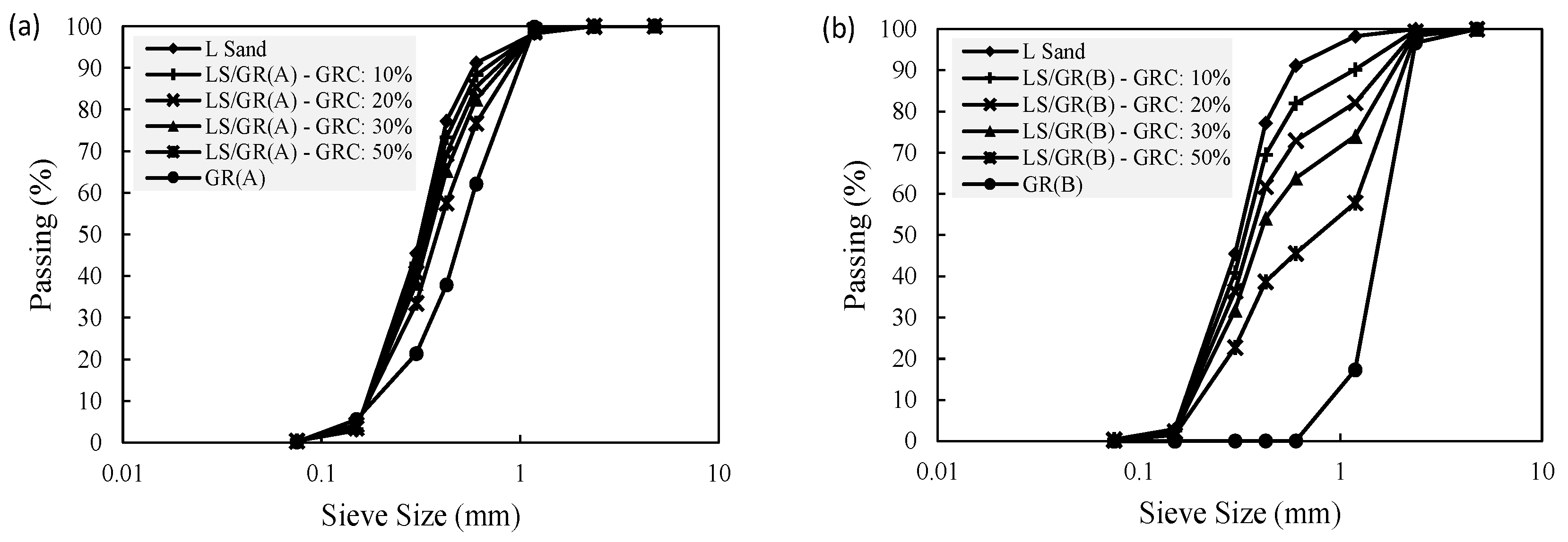
2.1. Materials

A subangular-shaped sand (L-Sand) with a Heywood circularity factor (HCF) of 1.10 was used in this experiment. It is a poorly graded sand with a specific gravity of 2.57 and a mean particle size of 0.32 mm. The density of the sand was 1507 kg/m3 at its minimum and 1751 kg/m3 at its maximum. The maximum density is achieved by using the vibratory table [30], whereas the minimum density is achieved by dropping the granular particle from a very low high distance (zero height). HCF is defined as follows:
H C F = P a r t i c l e   p e r i m e t e r 2 × π × P a r t i c l e   a r e a
Two sizes of granular rubber were provided by the Tyre Cycle Company in Melbourne, Victoria. Figure 1 shows the particle size distribution of used sand with the granular rubber-A (GR-A) and granular rubber-B (GR-B) at different percentages.
The characteristics of the used materials are summarized in Table 1. GR-A is composed of particles whose sizes range between 0.057 and 2.36 mm, with a mean particle size (D50) of 0.51 mm, while GR-B is composed of particles whose sizes range from 0.6 to 4 mm with D50 of 1.67 mm. GR-A had an HCF of 1.38 and a specific gravity of 0.99. The size ratio (SR) of rubber A and B were 1.59 and 5.22, respectively. As the granular rubber percentage in the mixtures increased, both the coefficients of uniformity (Cu) and the coefficients of curvature (Cc) increased, whereas the mixture unit weight decreased. The reason for this is that sand and granular rubber have different mean particle sizes; adding them together at specific percentages could produce a well-graded mixture.

2.2. Direct Shear Test

This study utilized direct shear test equipment made by Matest company. In this device, vertical and horizontal forces were applied and measured with an accuracy of 0.001 N. Additionally, horizontal, and vertical displacements were measured with an accuracy of 0.001 mm. A horizontal displacement rate of 1 mm per minute was applied in this study. A schematic diagram of the direct shear test is shown in Figure 2. The experiment was carried out on a direct shear box (60 × 60 mm) following the Australian standard [64].

2.3. Sample Preparation

Granular rubber was added to the sand at different percentages in this study. Using Equation (2), the granular rubber content (GRC) was used as a parameter to calculate the rubber content in different sand–rubber mixtures. In this study, mixtures with a GRC of 0, 10, 20, 30 and 50% were prepared. Before pouring each sample into the mold, each sample was thoroughly mixed.
G R C = M G R M T o t a l
where GRC is granular rubber content, MGR is mass of granular rubber, and Mtotal is mass of mixture (granular rubber and sand). The effect of the sand–rubber mixture density on shear strength and friction angle was also investigated. For this purpose, three different densities were considered: loose, slightly dense, and dense states. Each density state was achieved by applying a specific amount of compression energy [65]. Equation (3) was used to determine the amount of energy applied to each sample.
E = N b l o w s . N l a y e r s . W h a m m e r . H d r o p V m o l d
where E is input compaction energy, Nblows is the number of blows per layer, Nlayers is the number of compaction layers, Whammer is weight of hammer, Hdrop is height of hammer drop and Vmold is volume of mold. It is important to note that, in order to ensure a uniform distribution of granular rubber content throughout the mixture, the direct shear sample was meticulously prepared in layers. In a loose state, the sample was carefully placed from a very low height (zero high distance). For the slightly dense state, 165 kJ of energy was applied, and for the dense state, 825 kJ of energy was applied. Table 2 shows brief details of the compaction procedure for both slightly dense and dense states.
A shear zone is defined as the area where shear occurs, as shown in Figure 3. It is difficult to determine the exact amount of rubber in the shearing zone during sample preparation. To address this issue, samples were prepared in five layers, and the mixtures were divided into five different containers to ensure that the rubber quantity was distributed evenly across all layers and that the shear zone had approximately the correct rubber content.

2.4. Test Procedure

In this study, a total of 80 direct shear tests were conducted on L-Sand/GR (A) and L-Sand/GR (B) samples. The first group of tests were conducted at different states of density, varying from loose to slightly dense and dense states, along with different normal stresses of 30, 55, 105, and 200 kPa, and varying granular rubber contents of 0, 10, 20, 30, and 50%. The second group of tests were conducted at different densities, granular rubber contents, and normal stresses to investigate the impact of the size ratio. The direct shear tests were composed of two components: the application of normal stress, which varied over four levels, and horizontal displacement, which was applied at a rate of 1 mm/min.
Consistent with prior research on sand–rubber mixtures, dry specimens were used in this study to ensure consistency and comparability, with the focus on three main variables: normal stress, dry density, and granular rubber content. This decision was informed by the recognition that the shear strength of partially saturated soils often exceeds that of fully saturated or dry soils, making these the most unfavorable field conditions. However, compelling research conducted by Dai et al. [66] and Skinner [67] revealed that the discrepancy in shear strength between fully saturated and dry coarse materials is negligible. As a result, and given these considerations, we decided to carry out our experimental program under dry conditions. Consequently, pore water pressure was not measured in this experiment, as it was conducted on dry mixtures.
In the first stage of the experiment, in accordance with the Australian standards [64], normal stresses were applied to the specimens for 10 min to allow for consolidation before shear was initiated. Subsequently, shear stress was applied until the displacement reached 10 mm, which was equivalent to 15% of the specimen length, as per the standard requirements. Several tests were repeated to ensure the accuracy and repeatability of the results. Mathematical models were developed based on the obtained results to better understand the behavior of sand–rubber mixtures in response to various conditions of normal stress, dry density, and granular rubber content.

3. Mathematical Models

3.1. Multiple Linear Regression (MLR)

Multiple linear regression (MLR) analysis, as a statistical method, is beneficial as a prerequisite to exploring and comprehending other statistical or machine learning methodologies. This method is capable of predicting an output (dependent) variable based on two or more independent input variables. Simple linear regression (SLR) is another method that can predict one output (dependent) parameter based on only one input parameter. Equations (4) and (5) represents the typical linear equation for SLR and MLR, respectively.
y = β 0 + β 1 X + ε
y = β 0 + β 1 X 1 + β 2 X 2 + β 3 X 3 + β n X n + ε
where y is the output (dependent) parameter, X is the independents parameter, ε , β0, β1, β2, β3 and βn are constants or intercepts, X1, X2, X3, Xn are inputs (independent) parameters and n is the number of inputs.

3.2. Classification and Regression Random Forests (CRRF)

In 2001, Breiman introduced the amalgamation of random forest (RF) with decision trees [68]. To mitigate classification and regression errors, techniques such as bootstrap aggregation [69] and bagging [70] were employed in conjunction with decision trees. Through boosting, greater emphasis is placed on rectifying previously misclassified predictions, thereby promoting a more balanced prediction outcome. Meanwhile, by employing bagging, trees can be independently constructed using bootstrap samples from the dataset, as opposed to relying on reconstructions from preceding trees. As proposed by Breiman [68], random forests add an extra level of randomness to bagging by predicting the outcome based on a simple majority vote. A random forest constructs classification and regression trees differently based on different bootstrap data samples. Standard trees are partitioned into nodes based on the best split among all variables. A random selection of predictors is used to divide each node into random forests. This approach is quite effective in comparison to a number of other classification methods, such as discriminant analysis, support vector machines, and neural networks, as well as being resistant to overfitting [68]. Furthermore, this method is user-friendly and is insensitive to the number of random variables in the node and the number of trees in the forest.

3.3. Genetic Programing (GP)

There are many well-known algorithms that belong to the category of evolutionary algorithms, and one of the most well-known is genetic programming (GP). The origin of this algorithm can be traced back to Cramer [71] who created it, inspired by Darwin’s principle of “survival of the fittest”. It was then improved by Koza [72]. A number of applications for GP can be found, including curve fitting, data modelling, symbolic regression, feature selection, classification and so on. Over the past decade, GP has been used to solve complex real-world problems in a variety of fields [73,74,75]. Computer programs (CPs) in GP are binary-coded strings that follow the LISP programming language [76]. Parse trees can be derived from these solutions in a variety of sizes and shapes. GP solutions include terminals (e.g., input variables and constants) and calculations (e.g., +, −, ×, /, and other complex functions). Based on the nature of the problem and existing study proposals, mathematical functions are usually defined. By using mutation, crossover, and reproduction operators, GP can explore the search space and find a global optimal solution [76].

4. Results

4.1. Experimental

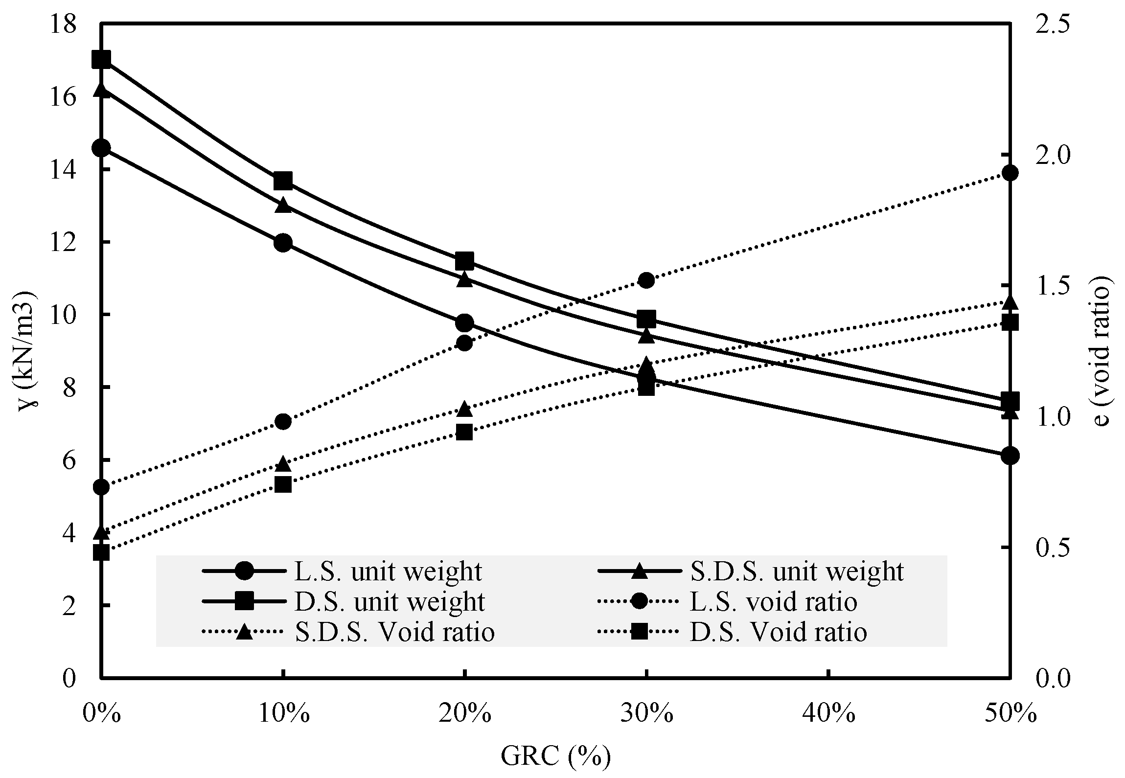
4.1.1. Unit Weight, and Void Ratio

A parameter that is strongly affected by the amount of rubber is the unit weight of the sand–rubber mixture. In general, since rubber has a lower specific gravity than sand, the unit weight of the mixture is expected to decrease with an increased amount of rubber. Figure 4 shows the unit weight results of different mixtures containing different percentages of granular rubber. The results indicated that the unit weight of the mixture decreased from approximately 17 kN/m3 to approximately 7.6 kN/m3 when the amount of rubber was increased from 0 to 50% in the dense state. With increasing amounts of rubber, with the same compaction energy (density or void ratio), the unit weight of the sand–rubber mixture decreased.
The soil void ratio is another parameter which is very important. To calculate the soil void ratio, the following equations are used:
e = V v o i d V s o l i d
e = V m W S G S + W P R G P R W S G S + W P R G P R
where e is the void ratio, Vvoid is the volume of voids in sand–rubber mixture, Vsolid is the volume of solid portion in sand–rubber mixture, Vm is the volume of mold, WPR is the weight of rubber, WS is the weight of sand, GS is the specific gravity of sand, and GPR is the specific gravity of rubber. According to the results, the void ratio increased with increasing GRC under various density states. This is due to the fact that granular rubber has a more irregular shape than sand particles, which can result in extra void spaces between the particles, increasing the total void ratio in the mixture.

4.1.2. Shear Strength

The effect of the amount of rubber on the shear strength of the sand–rubber mixture will have a significant impact on geotechnical designs. The preliminary results of the direct shear test to determine shear strength are shown in Figure 5, Figure 6 and Figure 7 for the loose, slightly dense, and dense states, respectively. For different normal stresses and different rubber contents, two types of graphs are presented, i.e., shear strength versus horizontal displacement and vertical displacement versus horizontal displacement.
According to Figure 5, in the loose state, almost all samples with different rubber contents and different normal stresses do not exhibit a peak in the shear strength versus the horizontal displacement diagram, and the diagrams correspond to the typical behavior of loose soils. The figure also shows that all samples displayed contraction behaviour during the shear test. The results also indicated that, in the loose state, and at different normal stresses, the 50% rubber content had the lowest shear strength, although the difference was not significant. Furthermore, the results indicated that under normal stress conditions of 55, 105, and 200 kPa, the highest shear strengths were achieved with sand–rubber mixtures containing 30, 20, and 20% granular rubber content, respectively.
Figure 6 illustrates the results of the direct shear test in the slightly dense state. The results show that sand–rubber mixtures with 0 and 10% rubber content showed a peak in the shear strength versus the horizontal displacement graph under normal stresses of 200 kPa and 105 kPa, respectively, and sand–rubber mixtures with 0% rubber content showed a peak under normal stresses of 55 kPa. Moreover, the results showed that the sand–rubber mixture with zero percentage of rubber exhibited a dilation behavior under normal stresses of 55, 105, and 200 kPa, while sand–rubber mixtures with 10% rubber content dilated under normal stresses of 55 and 105 kPa but contracted under other normal stresses.
Figure 7 illustrates the results of direct shear tests conducted on sand–rubber mixtures in a dense state (low void ratio). The results indicated that the amount of dilation and contraction depended on different parameters, such as the normal stress, mixture unit weight, and rubber content. At all three normal stresses of 200, 105, and 55 kPa, sand–rubber mixtures with zero and 10% rubber contents demonstrated a peak in the shear strength-horizontal displacement diagram. The sand–rubber mixture with 0% rubber showed dilation behavior under all three normal stresses of 200, 105, and 55 kPa. The sand–rubber mixture with 10% rubber also showed a dilation behavior under 105 and 55 kPa normal stresses. The remaining conditions demonstrated contraction behavior in sand–rubber mixtures.
Figure 8 illustrates shear strength at different normal stresses (30, 55, 105, and 200 kPa), granular rubber content (0, 10, 20, 30, and 50%), and density states (loose, slightly dense, and dense). According to the trend line for each mixture in three different densities, the shear strength increases with an increase in dry density.

4.1.3. Internal Friction Angle

One of the most important aspects of this study is the calculation of the internal friction angle of sand–rubber mixtures. The laboratory experiment demonstrated that when the applied normal stress is negligible (zero), the shear strength of the mixture is almost zero (similar to sand), indicating that the sand–rubber mixture is a cohesionless mixture. The Mohr–Coulomb criteria (Equation (8)), which is intended for incompressible soil (rigid particles), is a linear relationship between applied normal stress and shear strength. To put it differently, the points of intersection between different applied normal stresses and their shear strength values share the same internal friction angle. In contrast, for sand–rubber mixtures, as the applied normal stress increases the internal friction angle decreases (Figure 9). This is because rubbers are compressible materials (soft particles), and normal stress can compress them. Therefore, the internal friction angle depends on the applied normal stress on the sand–rubber mixture.
τ = c + σ n tan φ
where τ and σ n are shear and normal stress, and c and φ are the cohesion and internal friction angle of the soil.
Figure 10 illustrates how the internal friction angle was calculated for the sand–rubber mixtures in this study. Since the cohesion of sand–rubber mixture is zero, the origin of Figure 10 is point A. The second point, B, represents the new shear strength for the applied normal stress with coordinates σ1 and τ1. As a result, the friction angle was calculated for each point (A, B, C, D, and E).
This study investigated two internal friction angles: peak (φp) and residual friction angles (φr). The φp and φr are calculated using the peak and residual shear stress values shown on the schematic diagram (Figure 11). The friction angle is determined by intersecting the peak and residual shear stress values with the origin (0, 0) on the shear strength-normal stress diagram and by measuring the angle to the x-axis (Figure 10). The φp and φr parameters were determined for all density states in this study.
Figure 12 and Figure 13 present the results of φp and φr, respectively, for the different densities considered in this study. At all densities, the φp and φr decreased with increases in normal stress. In addition, the results indicate that, in the loose state, according to Figure 12a and Figure 13a the 20% rubber mixture had the highest φp and φr under different normal stresses. Furthermore, both φp and φr of the 50% rubber mixture were highly dependent on the normal stress, with the greatest decrease occurring as the normal stress increased. As a result, the behavior of mixtures of sand and rubber with a high percentage of rubber differs from those with a low percentage of rubber due to the compressibility of rubber.
For the slightly dense and dense states, Figure 12b,c and Figure 13b,c illustrate the results of the φp and φr. According to the results, the φp and φr of sand–rubber mixtures are strongly influenced by the intensity of normal stress. In sand–rubber mixtures with higher rubber percentages, the greatest reduction in φp and φr was observed as a result of an increase in normal stress. The sand–rubber mixture with 50% rubber in Figure 12c has a φp of 46 at a normal stress of 30 kPa, and it has the highest friction angle among the sand–rubber mixtures with different rubber percentages. The φp of the sand–rubber mixture with 50% rubber decreased to about 31 when the normal stress was increased to 200 kPa, and it had the lowest angle among all sand–rubber mixtures with different percentages of rubber.
Figure 14 illustrates the effect of the rubber content on the vertical displacement of shear strength. The results showed that at all density states, including loose (LO), slightly dense (SD) and dense (DE) states, an increase in the amount of rubber resulted in an increase in the shear strain associated with the shear strength.

4.1.4. Volume Compressibility

Compressibility is one of the most critical characteristics of sand–rubber mixtures. According to the literature, compressibility decreases with an increase in mixture density. The following Equation (9) was used to calculate the coefficient of volume compressibility (mv) of the mixtures based on Figure 15.
m v = Δ e 1 + e 0 1 σ v
where e 0 and Δ e are the initial void ratio and void ratio changes, respectively, σ v 0 and Δ σ v are the initial effective vertical stress and effective vertical stress changes, respectively, and m v is the coefficient of volume compressibility.
Figure 16 illustrates the results of the calculation of the volume compressibility coefficient for sand–rubber mixtures under various conditions. Based on the results, a high rubber content leads to a high-volume compression coefficient, whereas a low rubber content leads to a low volume compression coefficient. Furthermore, according to the results, dense mixtures have a lower compressibility while loose mixtures have a higher compressibility. According to Figure 17, the reason for this is that pure sand compressibility is a result of particle rearrangement, whereas sand–rubber mixture compressibility results from particle rearrangement and rubber-particle compressibility. Thus, the sand–rubber mixture has a greater volume compressibility coefficient than pure sand. In addition, the slope of changes in the volume compressibility coefficient due to soil density is higher in sand–rubber mixtures with a high percentage of rubber. The volume compressibility coefficient of sand–rubber mixtures containing zero percent rubber remains almost unchanged when soil density increases.

4.2. AI Modelling

4.2.1. Database Preparation

In order to employ artificial intelligence methods with the database, a random division of the database comprising 60 datasets was conducted into two distinct groups: the training database and the testing database. Specifically, the training database encompassed 80% of the data (48 datasets), while the testing database consists of the remaining 20% (12 datasets). Ideally, these two databases should be almost similar in order to demonstrate the accuracy of the model across a wide range of parameters. Table 3 and Table 4 provide statistical data for the training and testing databases, respectively. The statistical information of both training and testing databases has almost similar minimum, maximum, mean, and standard deviations.
In order to evaluate the accuracy of the different models, six parameters, the coefficient of determination (R2), mean absolute error (MAE), root mean square error (RMSE), mean-squared error (MSE), mean-squared logarithmic error (MSLE) and root mean-squared logarithmic error (RMSLE) were calculated using Equations (10)–(15).
R 2 = N x m X ¯ m x p X ¯ p N x m X ¯ m 2 N x p X ¯ p 2 2
M A E = N ( x m x p )   N
R M S E = N x m x p 2 N
M S E = N ( x m x p ) 2 N
M S L E = N ( log ( x m + 1 ) ( log ( x p + 1 ) ) 2 N
R M S L E = N ( log ( x m + 1 ) ( log ( x p + 1 ) ) 2 N
where xm, xp, x m ¯ , x p ¯ and N are the actual and predicted values, the average of the actual and predicted values, and the number of datasets, respectively. The best model is the model that has an R2 of 1 and an MAE, RMSE, MSE, MSLE, RMSLE equal to 0.
To prepare the database, linear normalization was used to distribute inputs and outputs values from 0 to 1 (Equation (16)). Normalization can improve the performance of AI methods.
x n = x i x m i n x m a x x m i n
where x i and x n are unnormalized and normalized variable values, and x m i n and x m a x are the minimum and maximum unnormalized variable values.

4.2.2. Multiple Linear Regression

In multiple linear regression (MLR), the Pearson parameter (r) is one of the most important parameters. The Pearson correlation coefficient, often referred to as Pearson’s r or simply the correlation coefficient, is a measure of the linear relationship between two variables. It quantifies the strength and direction of the linear association between two variables. When the Pearson parameter is close to zero, there is almost no linear relationship between the two parameters. Conversely, when the Pearson parameter is close to 1 or −1, there is a strong linear relationship between the two parameters. In addition, the Pearson correlation matrix is a matrix that displays the pairwise correlation coefficients between multiple variables. It provides a comprehensive overview of the correlations between each pair of variables in a dataset. Essentially, the Pearson correlation matrix is constructed by calculating the Pearson correlation coefficient between each pair of variables in a dataset. The resulting matrix allows for a visual representation of the interdependencies and relationships among the variables.
Table 5 illustrates the Pearson parameter (r) for different input and output parameters. According to the results, the highest value of the Pearson parameter between the inputs and outputs was found between the rubber content and peak friction angle parameters, was equal to 0.593. This indicates that there is no strong linear relationship between input and output parameters. Thus, more complex methods, such as those using artificial intelligence, were required.
In Figure 18, the predicted friction angles by the MLR model are compared with the actual values obtained from laboratory tests. It is evident from the results that the scatter of quantitative points is wide, which suggests that the model may be inaccurate.
Table 6 and Table 7 illustrate the accuracy of the MLR model based on different parameters for the training and testing databases and for both φp and φr. For predicting the φp of the model using the training database, the RMSE and R2 were equal to 3.151 and 0.664, respectively, and for predicting the φr, they were equal to 3.121 and 0.562. Based on the testing database, the RMSE and R2 values for predicting the φp were 3.025 and 0.676, respectively, while the RMSE and R2 values for predicting the φr were 2.844 and 0.604, respectively. According to these results, the MLR model was not capable of predicting the two outputs with high accuracy.

4.2.3. Genetic Programming

The genetic programming (GP) model was evaluated by changing the effective parameters in the model to determine the best and most optimal model. As a result, the best GP model with the specifications stated in Table 8 was selected. In the most accurate GP model, crossover was equal to 0.9 and the mutation parameter was equal to 0.99.
One of the influencing parameters in the accuracy and time of GP model is the size of the population. In the beginning, size was considered equal to 500. After a lot of trial and error, as shown in Figure 19, it was observed that 500 is a relatively high number for population size, and that after a population size of almost 180, the accuracy of the GP model did not significantly change. As a result, with a little approximation, 200 was chosen for the size of the population.
Based on the developed GP model, Figure 20 illustrates the predicted versus actual φp and φr parameters. According to the results, the model was able to predict both the φp and φr parameters accurately.
Equations (17) and (18) are the results of the best GP model. The inputs and outputs of the described functions should be normalized.
Ø p = r 2 2 r 3 G R C σ n + r 3 r 1 + σ n + r 3 r 1 σ n r 2 + [ γ d r 3 G R C + r 2 ]
Ø r = r 1 σ n r 2 + r 2 σ n 2 r 3 + G R C r 4 + γ d r 4 σ n
where GRC is the granular rubber content, σ n is normal stress, γ d is soils unit weight, φp and φr are the peak and residual internal friction angles, and r 1 , r 2 , r 3 and r 4 are constants and can be found in Table 9.
The accuracy of GP model based on different parameters for predicting two parameters of φp and φr are shown in Table 10 and Table 11. Based on the training database, GP model was able to predict the φp with the RMSE and R2 of 1.958 and 0.870 and the φr with the RMSE and R2 of 1.747 and 0.863. In addition, GP model was able to predict the testing database with the RMSE and R2 of 1.186 and 0.950 for the φp parameter, and 1.433 and 0.899 for the φr parameter. In these results, the GP model was shown to be highly accurate in predicting both the φp and φr.

4.2.4. Classification and Regression Random Forest

Based on a series of analyses, the best CRRF model was identified. Table 12 presents the most important parameters in the CRRF model for the best and most optimal model. The number of trees is one of the most important and influential parameters concerning the time and accuracy of the CRRF model. Based on various analyses, a tree depth of 100 was determined to be the most optimal depth. Anther effective parameter is the tree max depth parameter, which can have a significant impact on the complexity, time, and accuracy of the CRRF model. Based on the results of the analysis, a tree max depth of seven was determined to be the most appropriate tree max depth for this database.
A comparison of the values predicted by the CRRF model versus the actual values obtained from the experimental tests is shown in Figure 21. According to the results, the CRRF model accurately predicted both the test and training databases.
Table 13 and Table 14 present the RMSE and R2 of the CRRF model for the training and testing databases. Based on the results, the CRRF model for the training database predicted the φp with an RMSE of 1.046 and an R2 of 0.963, whereas the CRRF model using the testing database predicted the φp with an RMSE of 1.121 and an R2 of 0.955. Moreover, the results showed that the RMSE and R2 of the CRRF model for predicting φr for the training database were 1.116 and 0.944, respectively, and for the testing database they were 1.193 and 0.930, respectively. According to these results, the CRRF model is highly accurate in predicting both the φp and φr parameters.

5. Discussion

5.1. Particle Morphology

Granular rubber is available in a variety of particle sizes, and shapes, which can affect shear strength. Several studies have been published in the literature that investigated the sand–rubber mixture at different size ratio (S.R.) [39,77,78,79]. To investigate the effect of SR on shear strength, two SRs were used. For two particulate rubber sizes in the experiments, the SRs were 1.59 and 5.22, respectively. As illustrated in Figure 22, the mixture with an SR equal to 5.22 had a higher shear strength than the mixture with an SR of 1.59 in the dense state and at a normal stress of 200 kPa. These results were compliant with the Rouhanifar experiment [77] where a higher SR produced higher shear strength.

5.2. Active Lateral Pressure

Building retaining walls to retain soil in a specific area is a very common method of construction in geotechnical engineering. To construct retaining walls, it is necessary to determine the lateral pressure. A practical example in the discussion of sand–rubber mixtures is the effect of their density on lateral pressure. Studies have shown that the low density of the sand–rubber mixture can have a positive effect on the lateral pressure [40]. The lateral pressure can be calculated using Equation (19) for different depths.
σ h = γ z 1 sin φ 1 + sin φ 2 c cos φ 1 + sin φ
where σ h is horizontal pressure, γ is the unit weight of soil, z is depth, φ is the internal friction angle of soil and, c is the soil cohesion. Lateral pressures were calculated for different densities in this study. It was assumed that the soil depth is one meter for this purpose. Figure 23 illustrates the results of the calculation for different densities. With an increase in rubber content in the mixture, the lateral pressure of the soil decreased. These results confirm that rubber-sand mixtures can be used in retaining walls as lightweight materials, which will help to reduce design costs.

5.3. Comparison of AI Models

Based on the testing database, and for both outputs (φp and φr), Table 15 compares the results of the different mathematical models. According to the obtained results, for predicting φp, the MLR method had the highest MAE, MSE, RMSE, MSLE and RMSLE, and the lowest R2, while the CRRF model had the lowest MAE, MSE, RMSE, MSLE and RMSLE, and highest R2. In addition, the MLR model had the weakest R2 prediction for φr, while the CRRF model had the best performance. The results suggest that both artificial intelligence models, namely CRRF and GP, are capable of accurately predicting both output parameters.

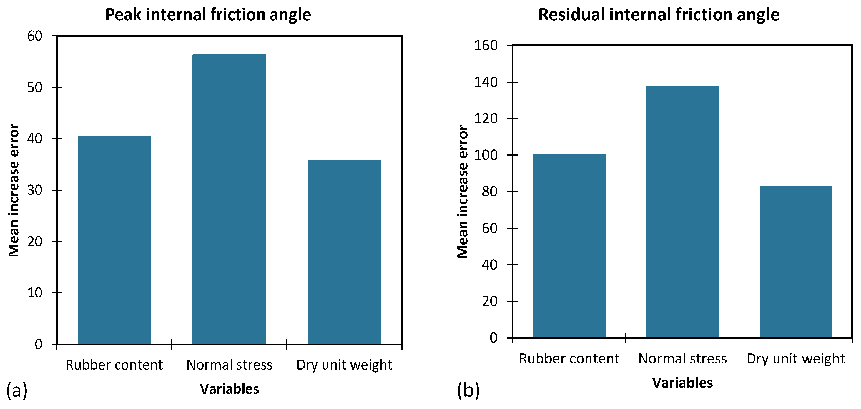
5.4. The Importance of Input Parameters

In artificial intelligence models, one of the most important debates is the importance of parameters. To determine the importance of each parameter, the values of the input parameters are individually increased and decreased by 100%, while the values of other input parameters are unchanged. The next step in our study was to calculate the error in the model caused by these changes. Figure 24 and Figure 25 illustrate the maximum errors created for each input parameter for the prediction of φp and φr, respectively. For both output parameters, normal stress had the highest error. This means that the models are more sensitive to changes in this parameter, so the importance of this parameter is high.
According to Table 16, both the φp and φr parameters are ranked in order of importance, where 1 indicates the most important and 3 indicates the least important. It was found that normal stress was the most significant factor in predicting both output parameters. The high importance of normal stress in predicting both output parameters could be explained by the fact that changes in normal stress can significantly affect the sand–rubber mixture density, as well as its shear strength and friction angle, which are key factors in resisting sliding under shear stress.
The observed difference in the importance rankings of rubber content and dry unit weight in the GP and CRRF models may be attributable to differences in their methodologies and learning approaches. GP relies on evolutionary algorithms and the evolution of program populations, whereas CRRF operates as an ensemble learning technique that combines multiple decision trees. These divergences in their techniques and internal mechanisms can contribute to divergent interpretations and rankings of the significance of input parameters.

6. Conclusions

Shear strength is an important parameter in geotechnical engineering that represents the ability of a soil to resist deformation when subjected to forces. The shear strength of a sand–rubber mixture is especially critical in geotechnical design as it determines the load-bearing capacity and stability of slopes, retaining structures, and foundations. The addition of rubber to sand improves its shear strength, making it a suitable material for construction on soft soils and for reducing the settling of structures built on it. Understanding the shear strength of sand–rubber mixtures is essential for ensuring the stability and longevity of geotechnical structures, and it is an important factor in the selection and design of appropriate construction materials and methods. The aim of this study was to examine the shear strength behavior of sand–rubber mixtures in direct shear tests. Two different sizes of rubber and one of sand were utilized, with the sand being mixed with various percentages of rubber (0%, 10%, 20%, 30%, and 50%). The mixtures were prepared in three states of density (loose, slightly dense, and dense), and shear stress was evaluated under four normal stress conditions (30, 55, 105, and 200 kPa). Below are a few highlights of the results:
  • The Mohr–Coulomb criteria cannot be effectively applied to sand–rubber mixtures as rubbers are compressible and the friction angle depends on normal stress, unlike incompressible soils where the friction angle remains constant with increases in normal stress;
  • A high rubber content results in a high-volume compression coefficient, while a low rubber content results in a low-volume compression coefficient. Dense mixtures have lower compressibility, while loose mixtures have higher compressibility;
  • The MLR model had low accuracy in predicting both φp and φr, with RMSE and R2 values of 3.151 and 0.664 for the training database, and 3.025 and 0.676 for the testing database for the φp, and 2.844 and 0.604 for the φr for the testing database;
  • Using the GP model, two equations to calculate φp and φr were proposed. The GP model achieved an RMSE of 1.958 and R2 of 0.870 for the φp and an RMSE of 1.747 and R2 of 0.863 for the φr based on the training database. The model also exhibited high accuracy in predicting the φp, with an RMSE of 1.186 and R2 of 0.950, and the φr, with an RMSE of 1.433 and R2 of 0.899 based on the testing database. These results demonstrate the exceptional predictive capability of the GP model for both the φp and φr;
  • The CRRF model accurately predicted φp with low RMSE and high R2 values for both the training (RMSE 1.046, R2 0.963) and testing (RMSE 1.121, R2 0.955) databases. The results showed high accuracy for φr predictions as well (training RMSE 1.116, R2 0.944, testing RMSE 1.193, R2 0.93);
  • The mixture with a size ratio of 5.22 had higher shear strength compared with the mixture with a size ratio of 1.59 under normal stresses of 200 kPa in a dense state;
  • An increase in rubber content in the mixture decreased lateral earth pressure, confirming that the sand–rubber mixture can be used as a lightweight material in retaining walls, thereby reducing costs;
  • The importance of parameters in AI models is determined by individually increasing/decreasing the values of input parameters and calculating the resulting error in the model. Results showed that normal stress had the highest error for both output parameters, indicating that the models are highly sensitive to changes in this parameter, making it the most important.

Author Contributions

Conceptualization, F.D., A.B. and H.A.N.; methodology, F.D. and A.B.; writing—original draft preparation, F.D. and A.B.; writing—review and editing, F.D., A.B., H.A.N. and R.S.F.; supervision, H.A.N. and R.S.F. All authors have read and agreed to the published version of the manuscript.

Funding

This research received no external funding.

Data Availability Statement

All data are available upon request to the author.

Conflicts of Interest

The authors declare no conflict of interest.

References

  1. Mohajerani, A.; Burnett, L.; Smith, J.V.; Markovski, S.; Rodwell, G.; Rahman, M.T.; Kurmus, H.; Mirzababaei, M.; Arulrajah, A.; Horpibulsuk, S. Recycling waste rubber tyres in construction materials and associated environmental considerations: A review. Resour. Conserv. Recycl. 2020, 155, 104679. [Google Scholar] [CrossRef]
  2. Qaidi, S.M.; Mohammed, A.S.; Ahmed, H.U.; Faraj, R.H.; Emad, W.; Tayeh, B.A.; Althoey, F.; Zaid, O.; Sor, N.H. Rubberized geopolymer composites: A comprehensive review. Ceram. Int. 2022, 48, 24234–24259. [Google Scholar] [CrossRef]
  3. Kole, P.J.; Löhr, A.J.; Van Belleghem, F.G.; Ragas, A.M. Wear and tear of tyres: A stealthy source of microplastics in the environment. Int. J. Environ. Res. Public Health 2017, 14, 1265. [Google Scholar] [CrossRef] [Green Version]
  4. Department of the Environment, Australian Government. Factsheet-Product Stewardship for End-of-Life Tyres. Available online: https://www.dcceew.gov.au/sites/default/files/documents/35159-fs-tps.pdf (accessed on 30 March 2023).
  5. Weldeslassie, T.; Naz, H.; Singh, B.; Oves, M. Chemical contaminants for soil, air and aquatic ecosystem. In Modern Age Environmental Problems and Their Remediation; Springer: Cham, Switzerland, 2018; pp. 1–22. [Google Scholar]
  6. Thomas, B.S.; Gupta, R.C. A comprehensive review on the applications of waste tire rubber in cement concrete. Renew. Sustain. Energy Rev. 2016, 54, 1323–1333. [Google Scholar] [CrossRef]
  7. Authority, E.P. Storage of Waste Tyres—Regulatory Impact Statement (RIS); EPA Victoria: Brisbane, Australia, 2014. [Google Scholar]
  8. Daghistani, F.; Naga, H.A. Shear Strength Characteristics of Sand-Particulate Rubber Mixture. Int. J. Geotech. Geol. Eng. 2023, 17, 36–41. [Google Scholar]
  9. Humphrey, D.N. Civil engineering applications of tire shreds. In Proceedings of the Tire Industry Conference, Hilton Head Island, SC, USA, 1–3 March 1999; pp. 1–16. [Google Scholar]
  10. Baghbani, A.; Daghistani, F.; Naga, H.A.; Costa, S. Development of a Support Vector Machine (SVM) and a Classification and Regression Tree (CART) to Predict the Shear Strength of Sand Rubber Mixtures. In Proceedings of the 8th International Symposium on Geotechnical Safety and Risk (ISGSR), Newcastle, Australia, 14 December 2022. [Google Scholar]
  11. Sahebzadeh, S.; Heidari, A.; Kamelnia, H.; Baghbani, A. Sustainability features of Iran’s vernacular architecture: A comparative study between the architecture of hot–arid and hot–arid–windy regions. Sustainability 2017, 9, 749. [Google Scholar] [CrossRef] [Green Version]
  12. Anvari, S.M.; Shooshpasha, I.; Kutanaei, S.S. Effect of granulated rubber on shear strength of fine-grained sand. J. Rock Mech. Geotech. Eng. 2017, 9, 936–944. [Google Scholar] [CrossRef]
  13. Baghbani, A.; Costa, S.; O’Kelly, B.C.; Soltani, A.; Barzegar, M. Experimental study on cyclic simple shear behaviour of predominantly dilative silica sand. Int. J. Geotech. Eng. 2023, 17, 91–105. [Google Scholar] [CrossRef]
  14. Zhang, T.; Cai, G.; Duan, W. Strength and microstructure characteristics of the recycled rubber tire-sand mixtures as lightweight backfill. Environ. Sci. Pollut. Res. 2018, 25, 3872–3883. [Google Scholar] [CrossRef]
  15. Lim, S.K.; Tan, C.S.; Li, B.; Ling, T.-C.; Hossain, M.U.; Poon, C.S. Utilizing high volumes quarry wastes in the production of lightweight foamed concrete. Constr. Build. Mater. 2017, 151, 441–448. [Google Scholar] [CrossRef]
  16. Bosscher, P.J.; Edil, T.B.; Kuraoka, S. Design of highway embankments using tire chips. J. Geotech. Geoenviron. Eng. 1997, 123, 295–304. [Google Scholar] [CrossRef]
  17. Lee, J.; Salgado, R.; Bernal, A.; Lovell, C. Shredded tires and rubber-sand as lightweight backfill. J. Geotech. Geoenviron. Eng. 1999, 125, 132–141. [Google Scholar] [CrossRef]
  18. O’Shaughnessy, V.; Garga, V.K. Tire-reinforced earthfill. Part 2: Pull-out behaviour and reinforced slope design. Can. Geotech. J. 2000, 37, 97–116. [Google Scholar] [CrossRef]
  19. Siddique, R.; Naik, T.R. Properties of concrete containing scrap-tire rubber—An overview. Waste Manag. 2004, 24, 563–569. [Google Scholar] [CrossRef] [PubMed]
  20. Lee, C.; Shin, H.; Lee, J.S. Behavior of sand–rubber particle mixtures: Experimental observations and numerical simulations. Int. J. Numer. Anal. Methods Geomech. 2014, 38, 1651–1663. [Google Scholar] [CrossRef]
  21. Heimdahl, T.C.; Drescher, A. Elastic anisotropy of tire shreds. J. Geotech. Geoenviron. Eng. 1999, 125, 383–389. [Google Scholar] [CrossRef]
  22. Yang, Z.; Zhang, Q.; Shi, W.; Lv, J.; Lu, Z.; Ling, X. Advances in properties of rubber reinforced soil. Adv. Civ. Eng. 2020, 2020, 6629757. [Google Scholar] [CrossRef]
  23. Meddah, A.; Merzoug, K. Feasibility of using rubber waste fibers as reinforcements for sandy soils. Innov. Infrastruct. Solut. 2017, 2, 5. [Google Scholar] [CrossRef]
  24. Feng, Z.-Y.; Sutter, K.G. Dynamic properties of granulated rubber/sand mixtures. Geotech. Test. J. 2000, 23, 338–344. [Google Scholar]
  25. Mahmoud, G. Shear strength characteristics of sand-mixed with granular rubber. Geotech. Geol. Eng. 2004, 22, 401–416. [Google Scholar]
  26. Poh, P.S.; Broms, B.B. Slope stabilization using old rubber tires and geotextiles. J. Perform. Constr. Facil. 1995, 9, 76–79. [Google Scholar] [CrossRef]
  27. Foose, G.J.; Benson, C.H.; Bosscher, P.J. Sand reinforced with shredded waste tires. J. Geotech. Eng. 1996, 122, 760–767. [Google Scholar] [CrossRef]
  28. Downs, L.A.; Humphrey, D.N.; Katz, L.E.; Rock, C.A. Water quality effects of using tire chips below the groundwater table. In Civil Engineering; University of Maine: Orono, ME, USA, 1996. [Google Scholar]
  29. Eldin, N.N.; Senouci, A.B. Rubber-tire particles as concrete aggregate. J. Mater. Civ. Eng. 1993, 5, 478–496. [Google Scholar] [CrossRef]
  30. ASTM. Standard Test Methods for Maximum Index Density and Unit Weight of Soils Using a Vibratory Table; ASTM: West Conshohocken, PA, USA, 2006. [Google Scholar]
  31. ASTM. Standard Terminology Relating to Rubber; ASTM: West Conshohocken, PA, USA, 2020. [Google Scholar]
  32. ASTM. Standard Practice for Use of Scrap Tires in Civil Engineering Applications; ASTM: West Conshohocken, PA, USA, 2020. [Google Scholar]
  33. Ahmed, I. Laboratory Study on Properties of Rubber-Soils; Purdue University: West Lafayette, IN, USA, 1993. [Google Scholar]
  34. Zornberg, J.G.; Cabral, A.R.; Viratjandr, C. Behaviour of tire shred sand mixtures. Can. Geotech. J. 2004, 41, 227–241. [Google Scholar] [CrossRef]
  35. Yoon, Y.W.; Heo, S.B.; Kim, K.S. Geotechnical performance of waste tires for soil reinforcement from chamber tests. Geotext. Geomembr. 2008, 26, 100–107. [Google Scholar] [CrossRef]
  36. Anbazhagan, P.; Manohar, D.; Rohit, D. Influence of size of granulated rubber and tyre chips on the shear strength characteristics of sand–rubber mix. Geomech. Geoeng. 2017, 12, 266–278. [Google Scholar] [CrossRef]
  37. Tian, Y.; Kasyap, S.S.; Senetakis, K. Influence of loading history and soil type on the normal contact behavior of natural sand grain-elastomer composite interfaces. Polymers 2021, 13, 1830. [Google Scholar] [CrossRef]
  38. Lee, J.-S.; Dodds, J.; Santamarina, J.C. Behavior of rigid-soft particle mixtures. J. Mater. Civ. Eng. 2007, 19, 179–184. [Google Scholar] [CrossRef] [Green Version]
  39. Li, W.; Kwok, C.Y.; Senetakis, K. Effects of inclusion of granulated rubber tires on the mechanical behaviour of a compressive sand. Can. Geotech. J. 2020, 57, 763–769. [Google Scholar] [CrossRef]
  40. Perez, J.L.; Kwok, C.; Senetakis, K. Micromechanical analyses of the effect of rubber size and content on sand-rubber mixtures at the critical state. Geotext. Geomembr. 2017, 45, 81–97. [Google Scholar] [CrossRef]
  41. Takano, D.; Chevalier, B.; Otani, J. Experimental and numerical simulation of shear behavior on sand and tire chips. In Proceedings of the 14th International Conference on Computer Methods and Recent Advances in Geomechanics, Kyoto, Japan, 22–25 September 2015; pp. 1545–1550. [Google Scholar]
  42. Noorzad, R.; Raveshi, M. Mechanical behavior of waste tire crumbs–sand mixtures determined by triaxial tests. Geotech. Geol. Eng. 2017, 35, 1793–1802. [Google Scholar] [CrossRef]
  43. Fakhimi, A.; Hosseinpour, H. The role of oversize particles on the shear strength and deformational behavior of rock pile material. In Proceedings of the 42nd US Rock Mechanics Symposium (USRMS), San Francisco, CA, USA, 29 June–2 July 2008. [Google Scholar]
  44. Ghazavi, M.; Ghaffari, J.; Farshadfar, A. Experimental determination of waste tire chip-sand-geogrid interface parameters using large direct shear tests. In Proceedings of the 5th Symposium on Advances in Science and Technology, Mashhad, Iran, 12–17 May 2011; pp. 12–17. [Google Scholar]
  45. Baghbani, A.; Choudhury, T.; Costa, S.; Reiner, J. Application of artificial intelligence in geotechnical engineering: A state-of-the-art review. Earth-Sci. Rev. 2022, 228, 103991. [Google Scholar] [CrossRef]
  46. Baghbani, A.; Nguyen, M.D.; Alnedawi, A.; Milne, N.; Baumgartl, T.; Abuel-Naga, H. Improving soil stability with alum sludge: An AI-enabled approach for accurate prediction of California Bearing Ratio. Appl. Sci. 2023, 13, 4934. [Google Scholar] [CrossRef]
  47. Essam, Y.; Kumar, P.; Ahmed, A.N.; Murti, M.A.; El-Shafie, A. Exploring the reliability of different artificial intelligence techniques in predicting earthquake for Malaysia. Soil Dyn. Earthq. Eng. 2021, 147, 106826. [Google Scholar] [CrossRef]
  48. Baghbani, A.; Choudhury, T.; Samui, P.; Costa, S. Prediction of secant shear modulus and damping ratio for an extremely dilative silica sand based on machine learning techniques. Soil Dyn. Earthq. Eng. 2023, 165, 107708. [Google Scholar] [CrossRef]
  49. Suman, S.; Khan, S.; Das, S.; Chand, S. Slope stability analysis using artificial intelligence techniques. Nat. Hazards 2016, 84, 727–748. [Google Scholar] [CrossRef]
  50. Baghbani, A.; Abuel-Naga, H.; Shirani Faradonbeh, R.; Costa, S.; Almasoudi, R. Ultrasonic Characterization of Compacted Salty Kaolin–Sand Mixtures Under Nearly Zero Vertical Stress Using Experimental Study and Machine Learning. Geotech. Geol. Eng. 2023, 41, 2987–3012. [Google Scholar] [CrossRef]
  51. Baghbani, A.; Costa, S.; Choudhury, T. Developing Mathematical Models for Predicting Cracks and Shrinkage Intensity Factor during Clay Soil Desiccation. 2023. Available online: https://papers.ssrn.com/sol3/papers.cfm?abstract_id=4408164 (accessed on 30 March 2023).
  52. Nguyen, M.D.; Baghbani, A.; Alnedawi, A.; Ullah, S.; Kafle, B.; Thomas, M.; Moon, E.M.; Milne, N.A. Experimental Study on the Suitability of Aluminium-Based Water Treatment Sludge as a Next Generation Sustainable Soil Replacement for Road Construction. 2023. Available online: https://papers.ssrn.com/sol3/papers.cfm?abstract_id=4331275 (accessed on 30 March 2023).
  53. Hoang, N.-D.; Pham, A.-D. Hybrid artificial intelligence approach based on metaheuristic and machine learning for slope stability assessment: A multinational data analysis. Expert Syst. Appl. 2016, 46, 60–68. [Google Scholar] [CrossRef]
  54. Baghbani, A.; Costa, S.; Faradonbeh, R.S.; Soltani, A.; Baghbani, H. Modeling the effects of particle shape on damping ratio of dry sand by simple shear testing and artificial intelligence. Appl. Sci. 2023, 13, 4363. [Google Scholar] [CrossRef]
  55. Baghbani, A.; Costa, S.; Faradonbeh, R.S.; Soltani, A.; Baghbani, H. Experimental-AI investigation of the effect of particle shape on the damping ratio of dry sand under simple shear test loading. Appl. Sci. 2023, 13, 4363. [Google Scholar] [CrossRef]
  56. Baghbani, A.; Daghistani, F.; Baghbani, H.; Kiany, K. Predicting the Strength of Recycled Glass Powder-Based Geopolymers for Improving Mechanical Behavior of Clay Soils Using Artificial Intelligence; EasyChair: Manchester, UK, 2023. [Google Scholar]
  57. Baghbani, A.; Daghistani, F.; Baghbani, H.; Kiany, K.; Bazaz, J.B. Artificial Intelligence-Based Prediction of Geotechnical Impacts of Polyethylene Bottles and Polypropylene on Clayey Soil; EasyChair: Manchester, UK, 2023. [Google Scholar]
  58. Baghbani, A.; Daghistani, F.; Kiany, K.; Shalchiyan, M.M. AI-Based Prediction of Strength and Tensile Properties of Expansive Soil Stabilized with Recycled Ash and Natural Fibers; EasyChair: Manchester, UK, 2023. [Google Scholar]
  59. Choudhury, T.; Costa, S. Prediction of parallel clay cracks using neural networks–a feasibility study. In Contemporary Issues in Soil Mechanics: Proceedings of the 2nd GeoMEast International Congress and Exhibition on Sustainable Civil Infrastructures, Egypt 2018—The Official International Congress of the Soil-Structure Interaction Group in Egypt (SSIGE); Springer International Publishing: Cham, Switzerland, 2019; pp. 214–224. [Google Scholar]
  60. Baghbani, A.; Costa, S.; Choundhury, T.; Faradonbeh, R.S. Prediction of Parallel Desiccation Cracks of Clays Using a Classification and Regression Tree (CART) Technique. In Proceedings of the 8th International Symposium on Geotechnical Safety and Risk (ISGSR), Newcastle, Australia, 14 December 2022. [Google Scholar]
  61. Lawal, A.I.; Kwon, S. Application of artificial intelligence to rock mechanics: An overview. J. Rock Mech. Geotech. Eng. 2021, 13, 248–266. [Google Scholar] [CrossRef]
  62. Baghbani, A.; Baghbani, H.; Shalchiyan, M.M.; Kiany, K. Utilizing artificial intelligence and finite element method to simulate the effects of new tunnels on existing tunnel deformation. J. Comput. Cogn. Eng. 2022. [Google Scholar] [CrossRef]
  63. Tasalloti, A.; Chiaro, G.; Banasiak, L.; Palermo, A. Experimental investigation of the mechanical behaviour of gravel-granulated tyre rubber mixtures. Constr. Build. Mater. 2021, 273, 121749. [Google Scholar] [CrossRef]
  64. AS1289.6.2.2; Determination of Shear Strength of a Soil—Direct Shear Test Using a Shear Box. Standards Australia: Sydney, Australia, 2020.
  65. Senthen Amuthan, M.; Boominathan, A.; Banerjee, S. Density and shear strength of particulate rubber mixed with sand and fly ash. J. Mater. Civ. Eng. 2018, 30, 04018136. [Google Scholar] [CrossRef]
  66. Dai, B.B.; Yang, J.; Zhou, C.Y. Observed effects of interparticle friction and particle size on shear behavior of granular materials. Int. J. Geomech. 2016, 16, 04015011. [Google Scholar] [CrossRef]
  67. Skinner, A. A note on the influence of interparticle friction on the shearing strength of a random assembly of spherical particles. Geotechnique 1969, 19, 150–157. [Google Scholar] [CrossRef]
  68. Breiman, L. Random forests. Mach. Learn. 2001, 45, 5–32. [Google Scholar] [CrossRef] [Green Version]
  69. Pan, W. Shrinking classification trees for bootstrap aggregation. Pattern Recognit. Lett. 1999, 20, 961–965. [Google Scholar] [CrossRef]
  70. Breiman, L. Bagging predictors. Mach. Learn. 1996, 24, 123–140. [Google Scholar] [CrossRef] [Green Version]
  71. Cramer, N.L. A representation for the adaptive generation of simple sequential programs. In Proceedings of the First International Conference on Genetic Algorithms and Their Applications; Psychology Press: London, UK, 2014; pp. 183–187. [Google Scholar]
  72. Koza, J.R. Evolution of subsumption using genetic programming. In Proceedings of the First European conference on Artificial Life; MIT Press: Cambridge, MA, USA, 1992; pp. 110–119. [Google Scholar]
  73. Koza, J.R. Genetic Programming: On the Programming of Computers by Means of Natural Selection (Complex Adaptive Systems); A Bradford Book: Denver, CO, USA, 1993; Volume 1, p. 18. [Google Scholar]
  74. Koza, J.R. Genetic programming as a means for programming computers by natural selection. Stat. Comput. 1994, 4, 87–112. [Google Scholar] [CrossRef]
  75. Pour, A.F.; Faradonbeh, R.S.; Gholampour, A.; Ngo, T.D. Predicting ultimate condition and transition point on axial stress–strain curve of FRP-confined concrete using a meta-heuristic algorithm. Compos. Struct. 2023, 304, 116387. [Google Scholar] [CrossRef]
  76. Gholampour, A.; Gandomi, A.H.; Ozbakkaloglu, T. New formulations for mechanical properties of recycled aggregate concrete using gene expression programming. Constr. Build. Mater. 2017, 130, 122–145. [Google Scholar] [CrossRef]
  77. Rouhanifar, S.; Afrazi, M.; Fakhimi, A.; Yazdani, M. Strength and deformation behaviour of sand-rubber mixture. Int. J. Geotech. Eng. 2021, 15, 1078–1092. [Google Scholar] [CrossRef]
  78. Wang, C.; Deng, A.; Taheri, A. Three-dimensional discrete element modeling of direct shear test for granular rubber–sand. Comput. Geotech. 2018, 97, 204–216. [Google Scholar] [CrossRef]
  79. Neaz Sheikh, M.; Mashiri, M.; Vinod, J.; Tsang, H.-H. Shear and compressibility behavior of sand–tire crumb mixtures. J. Mater. Civ. Eng. 2013, 25, 1366–1374. [Google Scholar] [CrossRef]
Figure 1. Particle size distribution of sand mixed with: (a) GR-A at different percentages; and (b) GR-B at different percentages.
Geosciences 13 00197 g001
Figure 2. A schematic diagram of the direct shear test.
Geosciences 13 00197 g002
Figure 3. Schematic distribution of rubber particles in sand–rubber mixtures.
Geosciences 13 00197 g003
Figure 4. Unit weight and void ratio versus granular rubber content for three different densities (loose state, slightly dense state, and dense state).
Geosciences 13 00197 g004
Figure 5. Shear stress and vertical deformation versus horizontal displacement for loose mixtures at different normal stresses of: (a) 200 kPa; (b) 105 kPa; and (c) 55 kPa.
Geosciences 13 00197 g005
Figure 6. Shear stress and vertical deformation versus horizontal displacement for slightly dense mixtures at different normal stresses of: (a) 200 kPa; (b) 105 kPa; and (c) 55 kPa.
Geosciences 13 00197 g006
Figure 7. Shear stress and vertical deformation versus horizontal displacement for dense mixtures at different normal stresses: (a) 200 kPa; (b) 105 kPa; and (c) 55 kPa.
Geosciences 13 00197 g007
Figure 8. Shear strength versus dry density at different normal stresses and rubber contents.
Geosciences 13 00197 g008
Figure 9. Schematic diagram for nonlinear experimental results and linear Mohr–Coulomb criteria.
Geosciences 13 00197 g009
Figure 10. Calculation of sand–rubber internal friction angle.
Geosciences 13 00197 g010
Figure 11. A typical diagram of shear stress- horizontal displacement for direct shear test.
Geosciences 13 00197 g011
Figure 12. Peak friction angle versus normal stresses at zero cohesion on different density states of: (a) loose, (b) slightly dense; and (c) dense states.
Geosciences 13 00197 g012aGeosciences 13 00197 g012b
Figure 13. Residual friction angle versus normal stresses at zero cohesion on different density states of (a) loose; (b) slightly dense; and (c) dense states.
Geosciences 13 00197 g013
Figure 14. Shear displacement of sand–rubber mixtures at maximum shear stress at different densities and different normal stresses of: (a) 30 kPa normal stress; (b) 55 kPa normal stress; (c) 105 kPa normal stress; and (d) 200 kPa normal stress.
Geosciences 13 00197 g014
Figure 15. Calculation of volume compressibility coefficient.
Geosciences 13 00197 g015
Figure 16. The coefficient of volume compressibility versus dry density for sand with different granular rubber contents.
Geosciences 13 00197 g016
Figure 17. Schematic view of sand rubber deformation in comparison to pure sand deformation.
Geosciences 13 00197 g017
Figure 18. MLR prediction compared with actual results for: (a) φp, and (b) φr.
Geosciences 13 00197 g018
Figure 19. GP fitness simulation for the best GP model.
Geosciences 13 00197 g019
Figure 20. GP prediction parameters compared with actual parameters for: (a) φp; and (b) φr.
Geosciences 13 00197 g020
Figure 21. The actual values versus the predicted values of: (a) φp; and (b) φr, for the best CRRF for both the training and testing databases.
Geosciences 13 00197 g021
Figure 22. Shear strength versus GRC for two different SRs at 200 kPa normal stress (dense state).
Geosciences 13 00197 g022
Figure 23. Lateral pressure versus dry density of sand–rubber mixtures at different dry densities and normal stresses.
Geosciences 13 00197 g023
Figure 24. Variable importance, the increase in MAE for: (a) φp; and (b) φr based on the GP.
Geosciences 13 00197 g024
Figure 25. Variable importance, the increase in MAE for: (a) φp; and (b) φr based on the CRRF.
Geosciences 13 00197 g025
Table 1. Sand and rubbers properties [8].
L SandGR-ALS-GR(A)
10%
LS-GR(A)
20%
LS-GR(A)
30%
LS-GR(A)
50%
GR-BLS-GR(B)
10%
LS-GR(B)
20%
LS-GR(B)
30%
LS-GR(B)
50%
D10 (mm)0.170.190.180.180.180.180.930.180.180.190.21
D30 (mm)0.250.370.250.260.260.281.370.260.270.290.36
D50 (mm)0.320.510.330.340.350.391.670.340.370.400.81
D60 (mm)0.360.580.370.380.400.451.810.380.420.531.24
CU (mm)2.043.042.112.182.262.491.942.142.272.805.92
CC (mm)0.961.190.970.970.980.991.100.960.970.840.49
Gs2.570.992.412.252.101.781.082.422.272.121.83
SR-1.591.591.591.591.595.225.225.225.225.22
HCF *1.101.38---------
* The HCF was calculated based on an average of 50 particles.
Table 2. The compaction energy of the L-Sand/GR (A) mixture.
Type of Mixtures N b l o w s N l a y e r s W h a m m e r   ( kN ) H d r o p   ( m ) V m o l d   ( m 3 ) Density StateTotal Energy (kJ)
L-Sand/GR (A)130.0260.300.00013896Slightly dense165
530.0260.30Dense825
Table 3. The statistical information of training database.
VariableObservationsMinimumMaximumMeanStd. Deviation
Dry unit weight, (kN/m3)48618.9601742.7301142.927339.775
Rubber percentage (%)480.0000.5000.2210.183
Normal stress (kPa)4830.000200.00097.50065.736
Peak friction angle (°)4827.95051.68038.1655.495
Residual friction angle (°)4827.18649.09634.7214.768
Table 4. The statistical information of testing database.
VariableObservationsMinimumMaximumMeanStd. Deviation
Dry unit weight, (kN/m3)12785.1201650.9101115.758266.606
Rubber percentage (%)120.0000.5000.2170.134
Normal stress (kPa)1230.000200.00097.50067.940
Peak friction angle (°)1232.35048.87039.3475.548
Residual friction angle (°)1231.63845.66536.6424.718
Table 5. The Pearson matrix of inputs and outputs.
Dry Unit WeightRubber ContentNormal StressPeak Friction AngleResidual Friction Angle
Dry unit weight10.063−0.451−0.111−0.221
Rubber content0.0631−0.080−0.5930.526
Normal stress−0.451−0.08010.1760.340
Peak friction angle−0.111−0.5930.17610.672
Residual friction angle−0.2210.4260.3400.6721
Table 6. The performance of the best MLR model to predict the φp.
Performance MetricsTraining DatabaseTesting Database
MAE2.5022.661
MSE9.9299.150
RMSE3.1513.025
MSLE0.0060.005
RMSLE0.0780.073
R20.6640.676
Table 7. The performance of the best MLR model to predict the φr.
Performance MetricsTraining DatabaseTesting Database
MAE2.3292.382
MSE9.7408.087
RMSE3.1212.844
MSLE0.0070.006
RMSLE0.0850.076
R20.5620.604
Table 8. The properties of the optimal GP model.
PopulationProbability of GP OperationsSelectionTree Structure LevelRandom ConstantsGP Imp. Parameters
SizeInitializationCrossoverMutationReproductionElitismMethodTour SizeMax. InitialMax. OperationFrom-toCountBrood Size
200HalfHalf0.90.990.21Tournament Selection2440–1102
Table 9. Constant values in Equations (16) and (17).
ConstantsIn Equation (16) to Calculate φ p In Equation (17) to Calculate φ r
r10.180210.91961
r20.20660.34778
r30.982550.28656
r4-0.30767
Table 10. The performance of the best GP model to predict the φp.
Performance MetricsTraining DatabaseTesting Database
MAE1.5911.048
MSE3.8341.406
RMSE1.9581.186
MSLE0.0020.001
RMSLE0.0490.030
R20.8700.950
Table 11. The performance of the best GP model to predict the φr.
Performance MetricsTraining DatabaseTesting Database
MAE1.3001.114
MSE3.0512.054
RMSE1.7471.433
MSLE0.0020.002
RMSLE0.0450.040
R20.8630.899
Table 12. The specifications of the best CRRF.
Trees ParametersForest Parameters
Min. Node SizeMin. Son SizeMax DepthMtryCPSamplingSample SizeNumber of Trees
21720.00001Random with replacement48100
Table 13. The performance of the best CRRF model to predict the φp.
Performance MetricsTraining DatabaseTesting Database
MAE0.8930.910
MSE1.0931.256
RMSE1.0461.121
MSLE0.0010.001
RMSLE0.0270.025
R20.9630.955
Table 14. The performance of the best CRRF model to predict the φr.
Performance MetricsTraining DatabaseTesting Database
MAE1.0231.106
MSE1.2451.423
RMSE1.1161.193
MSLE0.0010.001
RMSLE0.0320.032
R20.9440.930
Table 15. The results of three mathematical models for testing database.
Performance MetricsPeak Friction Angle (φp)Residual Friction Angle (φr)
MLRCRRFGPMLRCRRFGP
MAE2.6610.9101.0482.3821.1061.114
MSE9.1501.2561.4068.0871.4232.054
RMSE3.0251.1211.1862.8441.1931.433
MSLE0.0050.0010.0010.0060.0010.002
RMSLE0.0730.0250.0300.0760.0320.040
R20.6760.9550.9500.6040.9300.899
Table 16. The results of importance analysis for both AI methods.
Rubber ContentNormal StressDry Unit Weight
GPCRRFGPCRRFGPCRRF
Ø p 231132
Ø r 231132
Disclaimer/Publisher’s Note: The statements, opinions and data contained in all publications are solely those of the individual author(s) and contributor(s) and not of MDPI and/or the editor(s). MDPI and/or the editor(s) disclaim responsibility for any injury to people or property resulting from any ideas, methods, instructions or products referred to in the content.

