


Applications of Ground-Based Infrared Cameras for Remote Sensing of Volcanic Plumes

 , ,
, ,  , , ,
, , ,
Abstract
:1. Introduction
- Estimation of volcanic cloud (or plume) temperature and optical thickness using a radiative transfer model.
- Volcanic plume speed using an optical flow algorithm.
- Estimation of height and ascent velocity of buoyant volcanic columns.
2. Ground-Based Thermal Infrared Sensing of Volcanoes
3. The Imaging InfraRed Camera (IIRc) System
4. Data Analysis
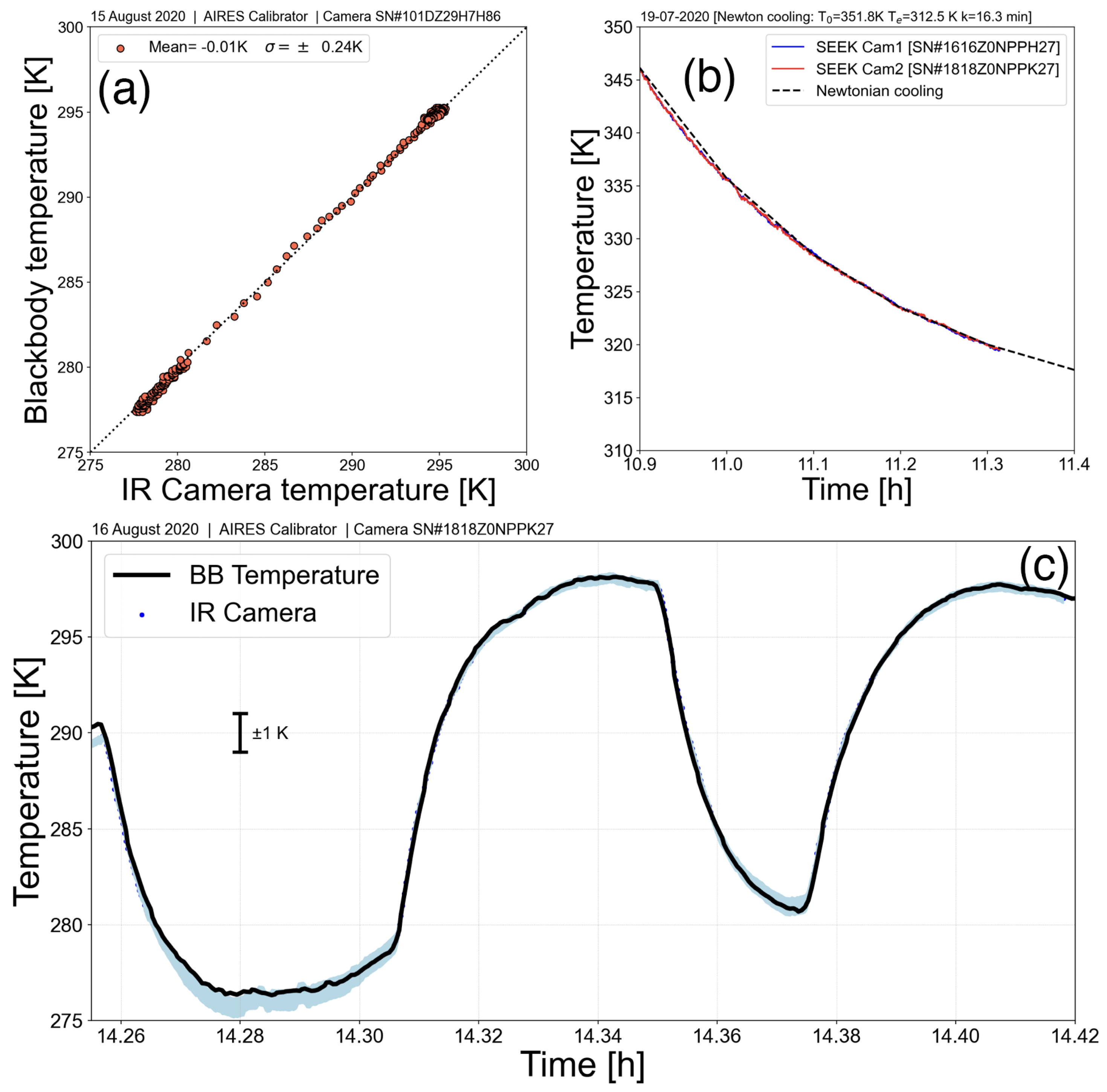
4.1. Calibration
4.2. Vignetting
4.3. Imaging Clear and Cloudy Skies
5. Radiative Transfer
6. Environmental Application: Volcanic Emissions
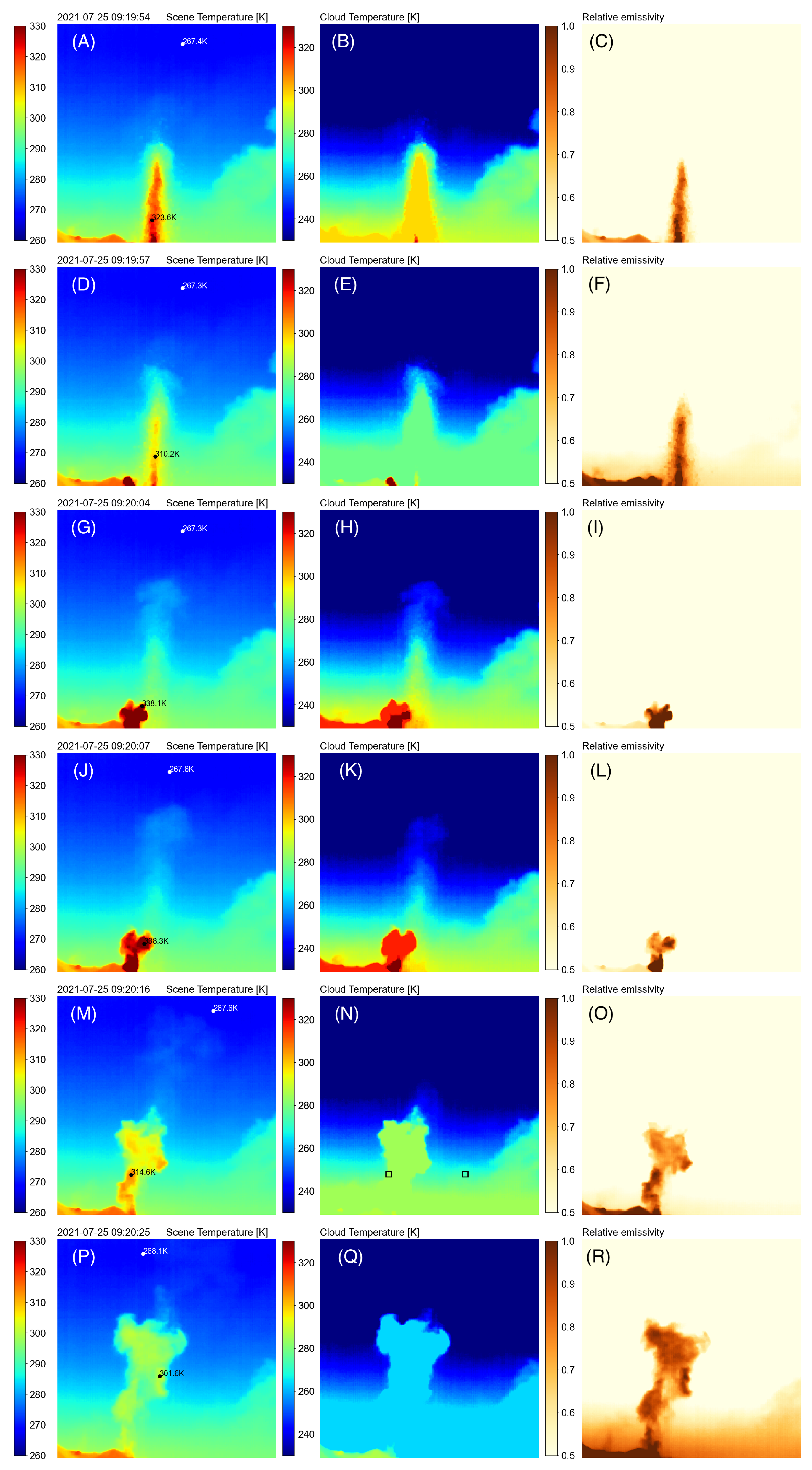
6.1. Cloud Temperature and Emissivity
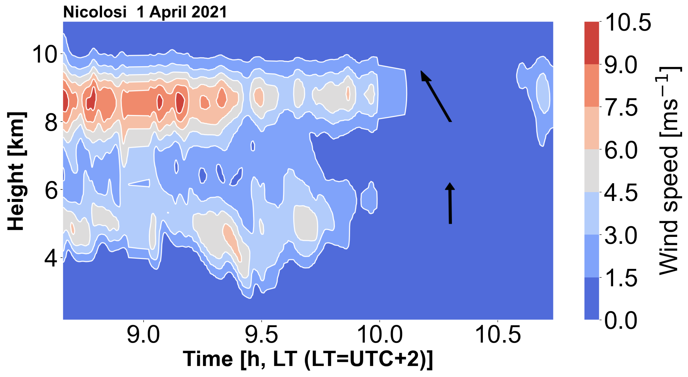
6.2. Optical Flow and Wind Speed
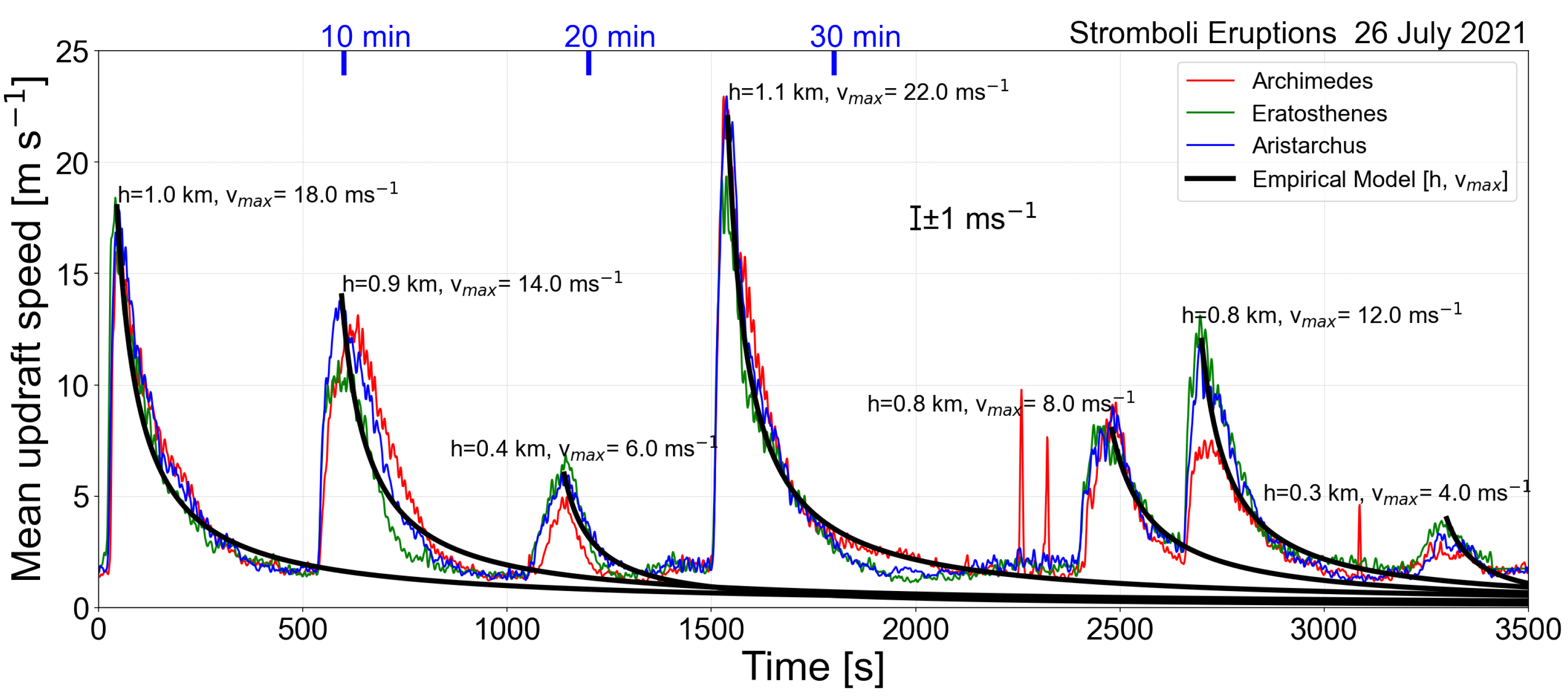
6.3. Height and Ascent Rate
7. Conclusions
Author Contributions
Funding
Institutional Review Board Statement
Informed Consent Statement
Data Availability Statement
Acknowledgments
Conflicts of Interest
Abbreviations
| COTS | Commerical Off-The-Shelf |
| FLIR | Forward-Looking Infra-Red |
| H2O | Water Vapour |
| HFOV | Horizontal Field Of View |
| INGV-VONA | Istituto Nazionale di Geofisica e Vulcanologia-Volcano Observatory Notices |
| for Aviation | |
| IR | InfraRed |
| IIRc | Imaging InfraRed camera |
| LED | Light-Emitting Diode |
| MEMS | Micro-ElectroMechanical System |
| MODTRAN | MODerate resolution atmospheric TRANsmission |
| NEDT | Noise Equivalent Temperature Difference |
| NUC | Non-Uniformity Correction |
| SBC | Single-Board Computer |
| SO2 | Sulfur Dioxide |
| VFOV | Vertical Field Of View |
References
- Kruse, P.W. Uncooled Thermal Imaging: Arrays, Systems, and Applications; SPIE Press: Bellingham, WA, USA, 2001; Volume 51. [Google Scholar]
- Blackett, M. An overview of infrared remote sensing of volcanic activity. J. Imaging 2017, 3, 13. [Google Scholar] [CrossRef]
- Oppenheimer, C.; Francis, P.W.; Rothery, D.A.; Carlton, R.W.; Glaze, L.S. Infrared image analysis of volcanic thermal features: Lascar Volcano, Chile, 1984–1992. J. Geophys. Res. Solid Earth 1993, 98, 4269–4286. [Google Scholar] [CrossRef]
- Harris, A. Thermal Remote Sensing of Active Volcanoes: A User’s Manual; Cambridge University Press: Cambridge, UK, 2013. [Google Scholar]
- Wright, R.; Flynn, L.P. On the retrieval of lava-flow surface temperatures from infrared satellite data. Geology 2003, 31, 893–896. [Google Scholar] [CrossRef]
- Ripepe, M.; Marchetti, E.; Poggi, P.; Harris, A.; Fiaschi, A.; Ulivieri, G. Seismic, acoustic, and thermal network monitors the 2003 eruption of Stromboli Volcano. Eos Trans. Am. Geophys. Union 2004, 85, 329–332. [Google Scholar] [CrossRef]
- Patrick, M.R.; Harris, A.J.; Ripepe, M.; Dehn, J.; Rothery, D.A.; Calvari, S. Strombolian explosive styles and source conditions: Insights from thermal (FLIR) video. Bull. Volcanol. 2007, 69, 769–784. [Google Scholar] [CrossRef]
- Patrick, M.R. Dynamics of Strombolian ash plumes from thermal video: Motion, morphology, and air entrainment. J. Geophys. Res. Solid Earth 2007, 112, B06202. [Google Scholar] [CrossRef]
- Sahetapy-Engel, S.T.; Harris, A.J. Thermal-image-derived dynamics of vertical ash plumes at Santiaguito volcano, Guatemala. Bull. Volcanol. 2009, 71, 827–830. [Google Scholar] [CrossRef]
- Prata, A.; Bernardo, C. Retrieval of volcanic ash particle size, mass and optical depth from a ground-based thermal infrared camera. J. Volcanol. Geotherm. Res. 2009, 186, 91–107. [Google Scholar] [CrossRef]
- Prata, A.J.; Bernardo, C. Retrieval of sulfur dioxide from a ground-based thermal infrared imaging camera. Atmos. Meas. Tech. 2014, 7, 2807–2828. [Google Scholar] [CrossRef]
- Vásconez, F.; Moussallam, Y.; Harris, A.J.; Latchimy, T.; Kelfoun, K.; Bontemps, M.; Macías, C.; Hidalgo, S.; Córdova, J.; Battaglia, J.; et al. VIGIA: A thermal and visible imagery system to track volcanic explosions. Remote Sens. 2022, 14, 3355. [Google Scholar] [CrossRef]
- Rowell, C.; Jellinek, A.; Gilchrist, J. Tracking Eruption Column Thermal Evolution and Source Unsteadiness in Ground-Based Thermal Imagery Using Spectral-Clustering. Geochem. Geophys. Geosyst. 2023, 24, e2022GC010845. [Google Scholar] [CrossRef]
- Mereu, L.; Marzano, F.S.; Bonadonna, C.; Lacanna, G.; Ripepe, M.; Scollo, S. Automatic early warning to derive eruption source parameters of paroxysmal activity at Mt. Etna (Italy). Remote Sens. 2023, 15, 3501. [Google Scholar] [CrossRef]
- Lopez, T.; Thomas, H.; Prata, A.; Amigo, A.; Fee, D.; Moriano, D. Volcanic plume characteristics determined using an infrared imaging camera. J. Volcanol. Geotherm. Res. 2015, 300, 148–166. [Google Scholar] [CrossRef]
- Fee, D.; Izbekov, P.; Kim, K.; Yokoo, A.; Lopez, T.; Prata, F.; Kazahaya, R.; Nakamichi, H.; Iguchi, M. Eruption mass estimation using infrasound waveform inversion and ash and gas measurements: Evaluation at Sakurajima Volcano, Japan. Earth Planet. Sci. Lett. 2017, 480, 42–52. [Google Scholar] [CrossRef]
- Li, H.; Zhu, M. Simulation of vignetting effect in thermal imaging system. In Proceedings of the SPIE—The International Society for Optical Engineering, Yichang, China, 30 October–1 November 2009; Volume 7494. [Google Scholar] [CrossRef]
- Berk, A.; Conforti, P.; Kennett, R.; Perkins, T.; Hawes, F.; Van Den Bosch, J. MODTRAN® 6: A major upgrade of the MODTRAN® radiative transfer code. In Proceedings of the 2014 6th Workshop on Hyperspectral Image and Signal Processing: Evolution in Remote Sensing (WHISPERS), Lausanne, Switzerland, 24–27 June 2014; pp. 1–4. [Google Scholar]
- Oppenheimer, C.; Kyle, P.R. Probing the magma plumbing of Erebus volcano, Antarctica, by open-path FTIR spectroscopy of gas emissions. J. Volcanol. Geotherm. Res. 2008, 177, 743–754. [Google Scholar] [CrossRef]
- Rizza, U.; Donnadieu, F.; Morichetti, M.; Avolio, E.; Castorina, G.; Semprebello, A.; Magazu, S.; Passerini, G.; Mancinelli, E.; Biensan, C. Airspace Contamination by Volcanic Ash from Sequences of Etna Paroxysms: Coupling the WRF-Chem Dispersion Model with Near-Source L-Band Radar Observations. Remote Sens. 2023, 15, 3760. [Google Scholar] [CrossRef]
- Farnebäck, G. Two-frame motion estimation based on polynomial expansion. In Proceedings of the Image Analysis: 13th Scandinavian Conference, SCIA 2003, Halmstad, Sweden, 29 June–2 July 2003; Proceedings 13. pp. 363–370. [Google Scholar]
- Thomas, H.E.; Prata, A. Computer vision for improved estimates of SO2 emission rates and plume dynamics. Int. J. Remote Sens. 2018, 39, 1285–1305. [Google Scholar] [CrossRef]
- Calvari, S.; Nunnari, G. Comparison between automated and manual detection of lava fountains from fixed monitoring thermal cameras at Etna Volcano, Italy. Remote Sens. 2022, 14, 2392. [Google Scholar] [CrossRef]
- Guerrieri, L.; Corradini, S.; Theys, N.; Stelitano, D.; Merucci, L. Volcanic Clouds Characterization of the 2020–2022 Sequence of Mt. Etna Lava Fountains Using MSG-SEVIRI and Products’ Cross-Comparison. Remote Sens. 2023, 15, 2055. [Google Scholar] [CrossRef]
- Scollo, S.; Prestifilippo, M.; Mereu, L. Estimations of eruption column height during Etna eruptions: A new database based on visible calibrated cameras. In Proceedings of the EGU General Assembly Conference Abstracts, Vienna, Austria, 23–28 April 2023; p. EGU–13071. [Google Scholar]
- Di Traglia, F.; Fornaciai, A.; Casalbore, D.; Favalli, M.; Manzella, I.; Romagnoli, C.; Chiocci, F.L.; Cole, P.; Nolesini, T.; Casagli, N. Subaerial-submarine morphological changes at Stromboli volcano (Italy) induced by the 2019–2020 eruptive activity. Geomorphology 2022, 400, 108093. [Google Scholar] [CrossRef]
- Rosi, M.; Pistolesi, M.; Bertagnini, A.; Landi, P.; Pompilio, M.; Di Roberto, A. Chapter 14 Stromboli volcano, Aeolian Islands (Italy): Present eruptive activity and hazards. Geol. Soc. Lond. Mem. 2013, 37, 473–490. [Google Scholar] [CrossRef]
- Calvari, S.; Lodato, L.; Steffke, A.; Cristaldi, A.; Harris, A.; Spampinato, L.; Boschi, E. The 2007 Stromboli eruption: Event chronology and effusion rates using thermal infrared data. J. Geophys. Res. Solid Earth 2010, 115, B04201. [Google Scholar] [CrossRef]


| Microbolomter | Uncooled VOx |
|---|---|
| Pixel pitch | 12 m |
| Spectral response | 7.8–14 m |
| Sensor resolution (H × V) | 320 × 240 |
| Frame rate | <9 Hz |
| Scene dynamic range | –40 °C to 330 °C |
| NET | 100 mK 25 °C |
| Non-uniformity correction (NUC) | automatic shutter |
| Video interface | USB |
| Supply voltage | 3.3V to 5.5V |
| Power (core only) | <50 mW |
| Power (core + interface) | 300 mW |
| Output formats | 16-bit or 32-bit floating point |
| Optics | |
| Focal length | 4 mm |
| Focus | Fixed |
| HFOV | 56° |
| VFOV | 42° |
| Mechanical | |
| Ingress protection | IP67 |
| Operating temperature range | −10 °C to 60 °C |
| Humidity | 10–95% (non-condensing) |
| Core dimensions (L × W × H) | 20 mm × 20 mm × 21 mm |
| Core weight | 12 g |
| Core material | Chalcogenide |
| Brand Name | ELP |
|---|---|
| Max. Resolution | 1260 × 960 (1.3 MP) |
| Model Number | ELP-USB4KHDR01-MFV (2.8–12 mm) |
| Auto Focus | No |
| Interface Type | USB |
| Sensor Type | 1/2.5 sony IMX317 sensor |
| Lens | 2.8–12 mm varifocal lens |
| High frame rate | 1260 × 960 MJPEG 30 fps |
| Output Formats | MJPEG, YUY2 |
| Minimal illumination: 0.2 Lux |
Disclaimer/Publisher’s Note: The statements, opinions and data contained in all publications are solely those of the individual author(s) and contributor(s) and not of MDPI and/or the editor(s). MDPI and/or the editor(s) disclaim responsibility for any injury to people or property resulting from any ideas, methods, instructions or products referred to in the content. |
© 2024 by the authors. Licensee MDPI, Basel, Switzerland. This article is an open access article distributed under the terms and conditions of the Creative Commons Attribution (CC BY) license (https://creativecommons.org/licenses/by/4.0/).
Share and Cite
Prata, F.; Corradini, S.; Biondi, R.; Guerrieri, L.; Merucci, L.; Prata, A.; Stelitano, D. Applications of Ground-Based Infrared Cameras for Remote Sensing of Volcanic Plumes. Geosciences 2024, 14, 82. https://doi.org/10.3390/geosciences14030082
Prata F, Corradini S, Biondi R, Guerrieri L, Merucci L, Prata A, Stelitano D. Applications of Ground-Based Infrared Cameras for Remote Sensing of Volcanic Plumes. Geosciences. 2024; 14(3):82. https://doi.org/10.3390/geosciences14030082
Chicago/Turabian StylePrata, Fred, Stefano Corradini, Riccardo Biondi, Lorenzo Guerrieri, Luca Merucci, Andrew Prata, and Dario Stelitano. 2024. "Applications of Ground-Based Infrared Cameras for Remote Sensing of Volcanic Plumes" Geosciences 14, no. 3: 82. https://doi.org/10.3390/geosciences14030082