

Analysis of Wildfire Susceptibility by Weight of Evidence, Using Geomorphological and Environmental Factors in the Marche Region, Central Italy

 , ,
, ,  and
and
Abstract
:1. Introduction
1.1. Worldwide Wildfire Situation and Trends
1.2. State of the Art Concerning Causal Factors and Fire Modelling
2. Materials and Methods
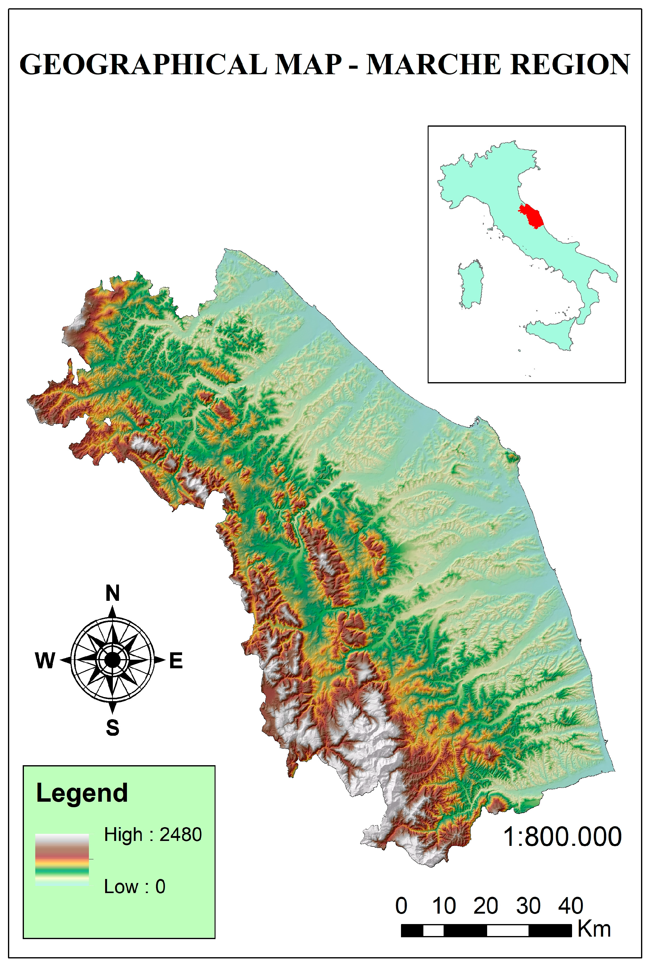
2.1. Study Area
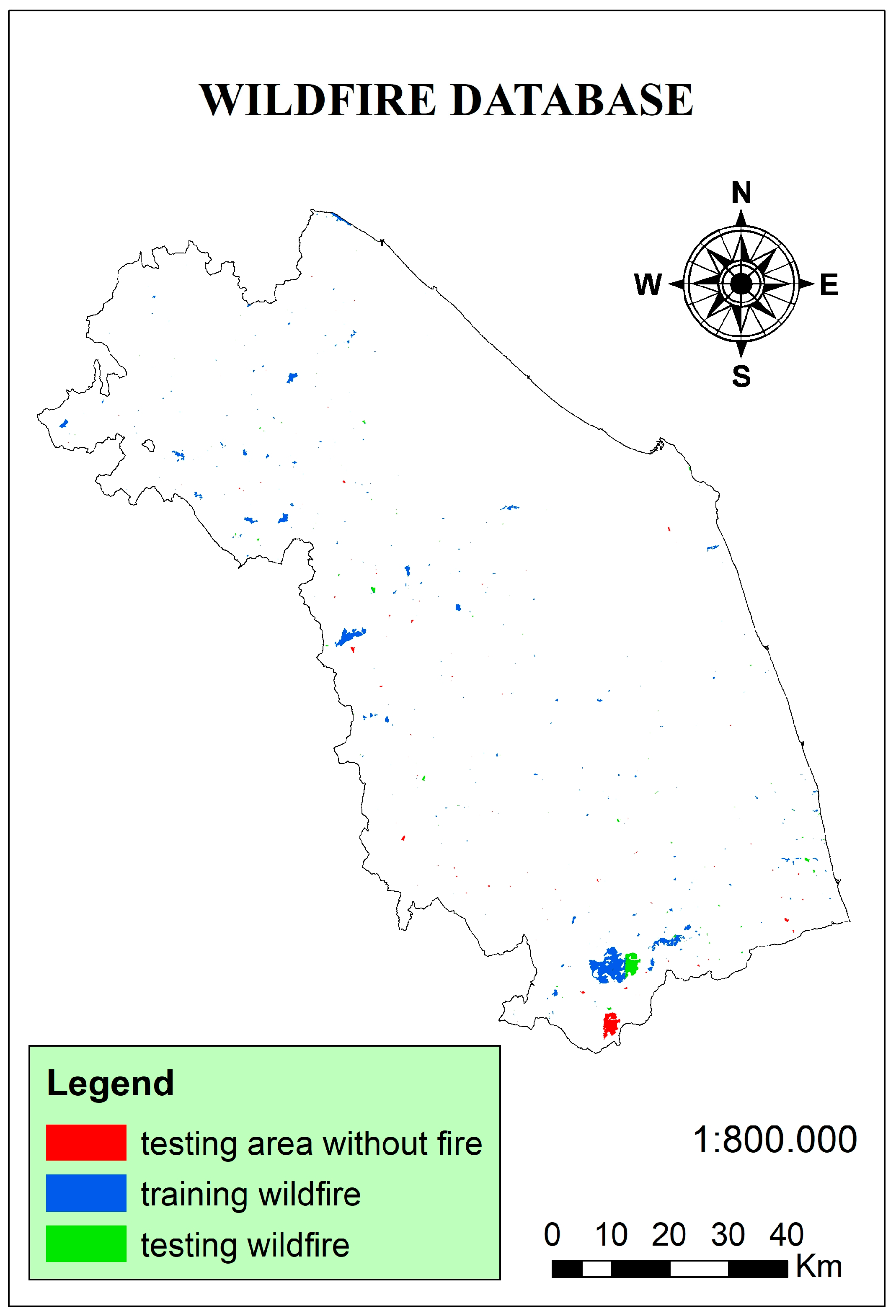
2.2. Data
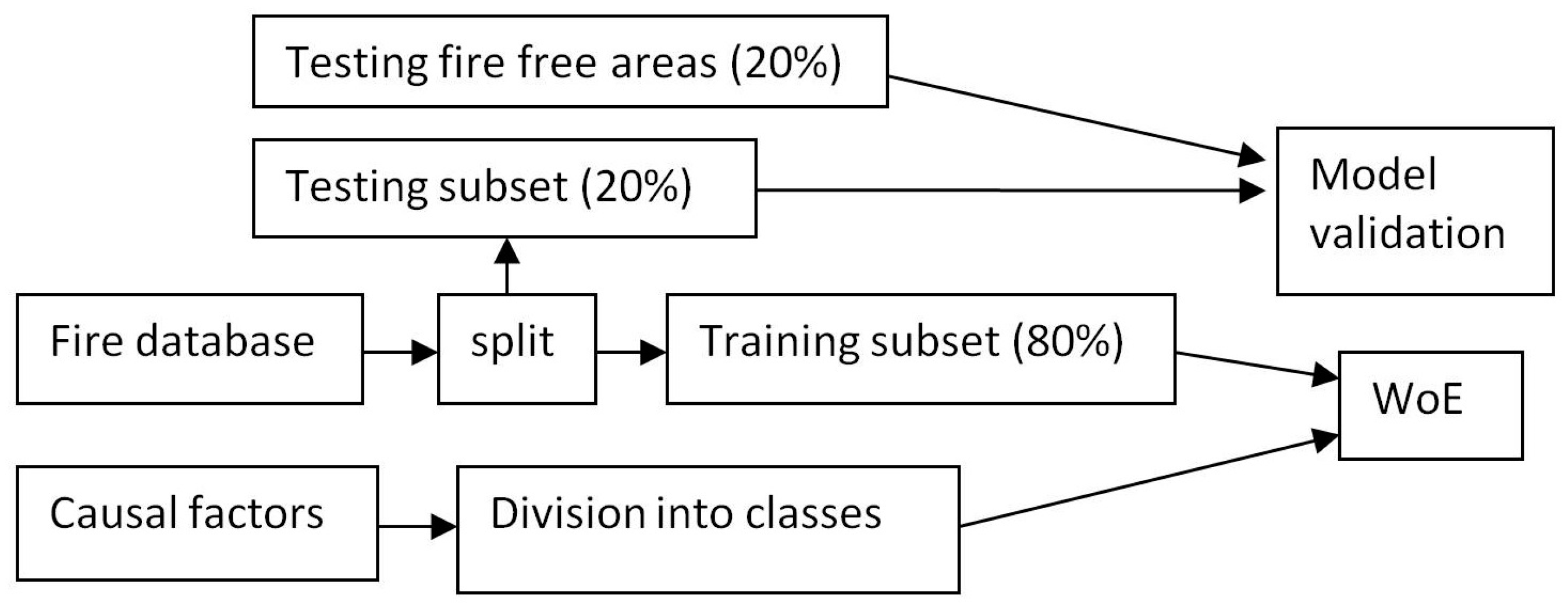
2.3. Methods
- AUC = 0.5 the test is not informative;
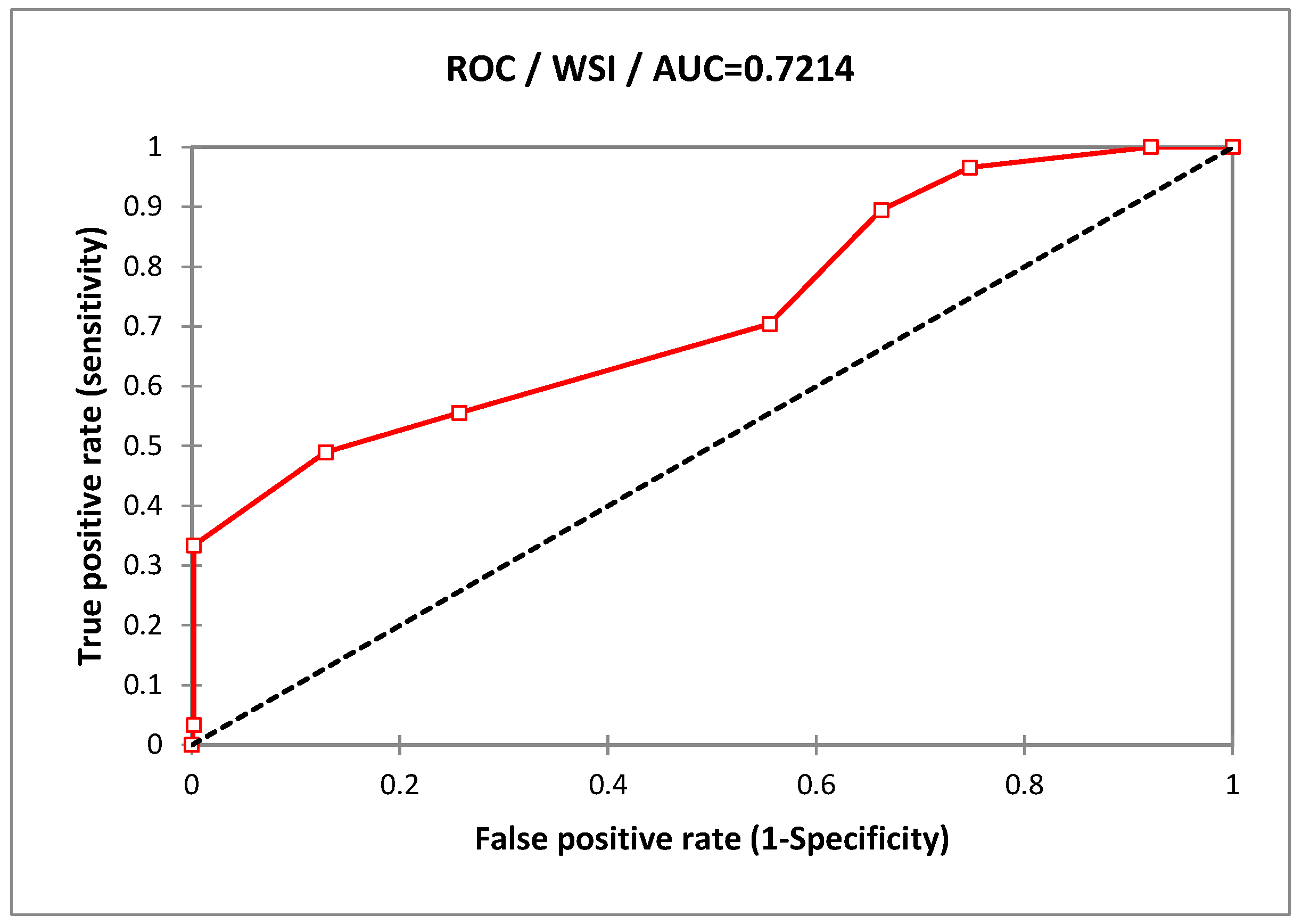
- 0.5 < AUC ≤ 0.7 the test is inaccurate;
- 0.7 < AUC ≤ 0.9 the test is highly accurate;
- 0.9 < AUC < 1.0, the test is considered outstanding;
- AUC = 1 perfect test.
3. Results
3.1. WoE Factors
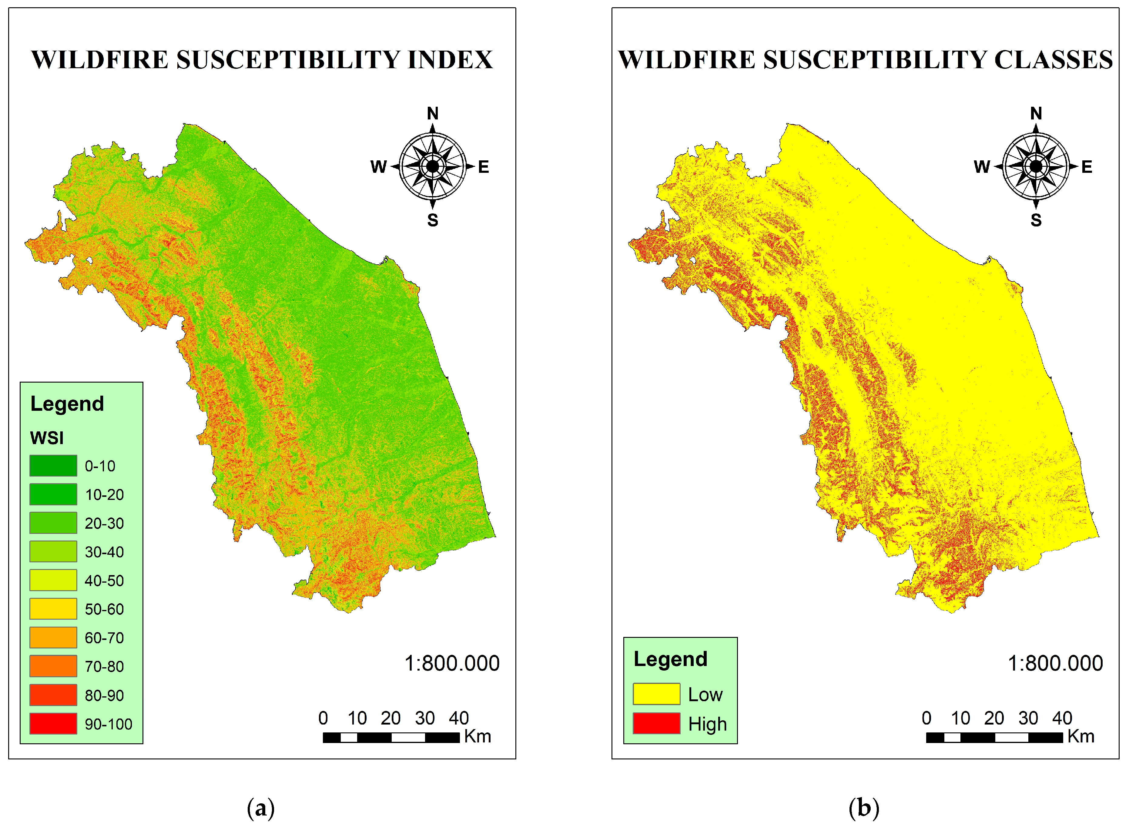
3.2. Wildfire Susceptibility and Model Validation
4. Discussion
5. Conclusions
Author Contributions
Funding
Data Availability Statement
Conflicts of Interest
References
- Collins, L.; Bradstock, R.A.; Clarke, H.; Clarke, M.F.; Nolan, R.H.; Penman, T.D. The 2019/2020 mega-fires exposed Australian ecosystems to an unprecedented extent of high-severity fire. Environ. Res. Lett. 2021, 16, 044029. [Google Scholar] [CrossRef]
- Syphard, A.D.; Keeley, J.E.; Gough, M.; Lazarz, M.; Rogan, J. What makes wildfires destructive in California? Fire 2022, 5, 133. [Google Scholar] [CrossRef]
- Garcia, L.C.; Szabo, J.K.; de Oliveira Roque, F.; Pereira, A.D.M.M.; da Cunha, C.N.; Damasceno-Júnior, G.A.; Morato, R.G.; Tomas, W.M.; Libonati, R.; Ribeiro, D.B. Record-breaking wildfires in the world’s largest continuous tropical wetland: Integrative fire management is urgently needed for both biodiversity and humans. J. Environ. Manag. 2021, 293, 112870. [Google Scholar] [CrossRef]
- Tedim, F.; Leone, V.; Coughlan, M.; Bouillon, C.; Xanthopoulos, G.; Royé, D.; Correia, F.J.M.; Ferreira, C. Extreme wildfire events: The definition. In Extreme Wildfire Events and Disasters; Elsevier: Amsterdam, The Netherlands, 2020; pp. 3–29. [Google Scholar]
- Weber, K.T.; Yadav, R. Spatiotemporal trends in wildfires across the Western United States (1950–2019). Remote Sens. 2020, 12, 2959. [Google Scholar] [CrossRef]
- Tomshin, O.; Solovyev, V. Spatio-temporal patterns of wildfires in Siberia during 2001–2020. Geocarto Int. 2022, 37, 7339–7357. [Google Scholar] [CrossRef]
- Ponomarev, E.; Yakimov, N.; Ponomareva, T.; Yakubailik, O.; Conard, S.G. Current trend of carbon emissions from wildfires in Siberia. Atmosphere 2021, 12, 559. [Google Scholar] [CrossRef]
- Larson-Nash, S.S.; Robichaud, P.R.; Pierson, F.B.; Moffet, C.A.; Williams, C.J.; Spaeth, K.E.; Brown, R.E.; Lewis, S.A. Recovery of small-scale infiltration and erosion after wildfires. J. Hydrol. Hydromech. 2018, 66, 261–270. [Google Scholar] [CrossRef]
- Ponomarev, E.I.; Kharuk, V.I.; Ranson, K.J. Wildfires dynamics in Siberian larch forests. Forests 2016, 7, 125. [Google Scholar] [CrossRef]
- Pausas, J.G.; Keeley, J.E. Wildfires and global change. Front. Ecol. Environ. 2021, 19, 387–395. [Google Scholar] [CrossRef]
- Burrows, N.D. Linking fire ecology and fire management in south-west Australian forest landscapes. For. Ecol. Manag. 2008, 255, 2394–2406. [Google Scholar] [CrossRef]
- Tonini, M.; D’Andrea, M.; Biondi, G.; Degli Esposti, S.; Trucchia, A.; Fiorucci, P. A machine learning-based approach for wildfire susceptibility mapping. The case study of the Liguria region in Italy. Geosciences 2020, 10, 105. [Google Scholar] [CrossRef]
- Leuenberger, M.; Parente, J.; Tonini, M.; Pereira, M.G.; Kanevski, M. Wildfire susceptibility mapping: Deterministic vs. stochastic approaches. Environ. Model. Softw. 2018, 101, 194–203. [Google Scholar] [CrossRef]
- Sayad, Y.O.; Mousannif, H.; Al Moatassime, H. Predictive modeling of wildfires: A new dataset and machine learning approach. Fire Saf. J. 2019, 104, 130–146. [Google Scholar] [CrossRef]
- Dilts, T.E.; Sibold, J.S.; Biondi, F. A weights-of-evidence model for mapping the probability of fire occurrence in Lincoln County, Nevada. Ann. Assoc. Am. Geogr. 2009, 99, 712–727. [Google Scholar] [CrossRef]
- Hislop, S.; Jones, S.; Soto-Berelov, M.; Skidmore, A.; Haywood, A.; Nguyen, T.H. Using landsat spectral indices in time-series to assess wildfire disturbance and recovery. Remote Sens. 2018, 10, 460. [Google Scholar] [CrossRef]
- Quesada-Román, A.; Vargas-Sanabria, D. A geomorphometric model to determine topographic parameters controlling wildfires occurrence in tropical dry forests. J. Arid Environ. 2022, 198, 104674. [Google Scholar] [CrossRef]
- Maniatis, Y.; Doganis, A.; Chatzigeorgiadis, M. Fire risk probability mapping using machine learning tools and multi-criteria decision analysis in the gis environment: A case study in the National Park Forest Dadia-Lefkimi-Soufli, Greece. Appl. Sci. 2022, 12, 2938. [Google Scholar] [CrossRef]
- Stambaugh, M.C.; Guyette, R.P. Predicting spatio-temporal variability in fire return intervals using a topographic roughness index. For. Ecol. Manag. 2008, 254, 463–473. [Google Scholar] [CrossRef]
- Carmo, M.; Moreira, F.; Casimiro, P.; Vaz, P. Land use and topography influences on wildfire occurrence in northern Portugal. Landsc. Urban Plan. 2011, 100, 169–176. [Google Scholar] [CrossRef]
- Vasilakos, C.; Kalabokidis, K.; Hatzopoulos, J.; Matsinos, I. Identifying wildland fire ignition factors through sensitivity analysis of a neural network. Nat. Hazards 2009, 50, 125–143. [Google Scholar] [CrossRef]
- Hostetler, S.W.; Bartlein, P.J.; Alder, J.R. Atmospheric and surface climate associated with 1986–2013 wildfires in North America. J. Geophys. Res. Biogeosciences 2018, 123, 1588–1609. [Google Scholar] [CrossRef]
- Nami, M.H.; Jaafari, A.; Fallah, M.; Nabiuni, S. Spatial prediction of wildfire probability in the Hyrcanian ecoregion using evidential belief function model and GIS. Int. J. Environ. Sci. Technol. 2018, 15, 373–384. [Google Scholar] [CrossRef]
- Jaafari, A.; Gholami, D.M.; Zenner, E.K. A Bayesian modeling of wildfire probability in the Zagros Mountains, Iran. Ecol. Inform. 2017, 39, 32–44. [Google Scholar] [CrossRef]
- Weed, D.L. Weight of evidence: A review of concept and methods. Risk Anal. Int. J. 2005, 25, 1545–1557. [Google Scholar] [CrossRef]
- Mohammed, O.A.; Vafaei, S.; Kurdalivand, M.M.; Rasooli, S.; Yao, C.; Hu, T. A Comparative Study of Forest Fire Mapping Using GIS-Based Data Mining Approaches in Western Iran. Sustainability 2022, 14, 13625. [Google Scholar] [CrossRef]
- Hong, H.; Naghibi, S.A.; Moradi Dashtpagerdi, M.; Pourghasemi, H.R.; Chen, W. A comparative assessment between linear and quadratic discriminant analyses (LDA-QDA) with frequency ratio and weights-of-evidence models for forest fire susceptibility mapping in China. Arab. J. Geosci. 2017, 10, 167. [Google Scholar] [CrossRef]
- Gentilucci, M.; Pambianchi, G. Prediction of Snowmelt Days Using Binary Logistic Regression in the Umbria-Marche Apennines (Central Italy). Water 2022, 14, 1495. [Google Scholar] [CrossRef]
- Gentilucci, M.; Burt, P. Using temperature to predict the end of flowering in the common grape (Vitis vinifera) in the Macerata wine region, Italy. Euro-Mediterr. J. Environ. Integr. 2018, 3, 38. [Google Scholar] [CrossRef]
- Gentilucci, M. Grapevine prediction of end of flowering date. In Recent Advances in Environmental Science from the Euro-Mediterranean and Surrounding Regions: Proceedings of Euro-Mediterranean Conference for Environmental Integration (EMCEI-1); Springer International Publishing: Cham, Switzerland, 2017; pp. 1231–1233. [Google Scholar]
- Bjånes, A.; De La Fuente, R.; Mena, P. A deep learning ensemble model for wildfire susceptibility mapping. Ecol. Inform. 2021, 65, 101397. [Google Scholar] [CrossRef]
- Gentilucci, M.; Rossi, A.; Pelagagge, N.; Aringoli, D.; Barbieri, M.; Pambianchi, G. GEV Analysis of Extreme Rainfall: Comparing Different Time Intervals to Analyse Model Response in Terms of Return Levels in the Study Area of Central Italy. Sustainability 2023, 15, 11656. [Google Scholar] [CrossRef]
- Gentilucci, M.; Barbieri, M.; Materazzi, M.; Pambianchi, G. Effects of Climate Change on Vegetation in the Province of Macerata (Central Italy). In Advanced Studies in Efficient Environmental Design and City Planning; Springer International Publishing: Cham, Switzerland, 2021; pp. 463–474. [Google Scholar]
- Gentilucci, M.; Pelagagge, N.; Rossi, A.; Aringoli, S.; Pambianchi, G. Landslide Susceptibility Using Climatic–Environmental Factors Using the Weight-of-Evidence Method—A Study Area in Central Italy. Appl. Sci. 2023, 13, 8617. [Google Scholar] [CrossRef]
- Singh, B.; Maharjan, M.; Thapa, M.S. Wildfire Risk Zonation of Sudurpaschim Province, Nepal. For. J. Inst. For. Nepal 2020, 17, 155–173. [Google Scholar] [CrossRef]
- Swets, J.A. Measuring the accuracy of diagnostic systems. Science 1988, 240, 1285–1293. [Google Scholar] [CrossRef]
- Mandrekar, J.N. Receiver operating characteristic curve in diagnostic test assessment. J. Thorac. Oncol. 2010, 5, 1315–1316. [Google Scholar] [CrossRef]
- Milanović, S.; Kaczmarowski, J.; Ciesielski, M.; Trailović, Z.; Mielcarek, M.; Szczygieł, R.; Kwiatkowski, M.; Bałazy, R.; Zasada, M.; Milanović, S.D. Modeling and mapping of forest fire occurrence in the Lower Silesian Voivodeship of Poland based on Machine Learning methods. Forests 2022, 14, 46. [Google Scholar] [CrossRef]
- Kooijman, A.M. Litter quality effects of beech and hornbeam on undergrowth species diversity in Luxembourg forests on limestone and decalcified marl. J. Veg. Sci. 2010, 21, 248–261. [Google Scholar] [CrossRef]
- Koontz, M.J.; North, M.P.; Werner, C.M.; Fick, S.E.; Latimer, A.M. Local forest structure variability increases resilience to wildfire in dry western US coniferous forests. Ecol. Lett. 2020, 23, 483–494. [Google Scholar] [CrossRef]
- Stavi, I. Wildfires in grasslands and shrublands: A review of impacts on vegetation, soil, hydrology, and geomorphology. Water 2019, 11, 1042. [Google Scholar] [CrossRef]
- Azevedo, J.C.; Possacos, A.; Aguiar, C.F.; Amado, A.; Miguel, L.; Dias, R.; Loureiro, C.; Fernandes, P.M. The role of holm oak edges in the control of disturbance and conservation of plant diversity in fire-prone landscapes. For. Ecol. Manag. 2013, 297, 37–48. [Google Scholar] [CrossRef]
- Dorji, S.; Ongsomwang, S. Wildfire susceptibility mapping in bhutan using geoinformatics technology. Suranaree J. Sci. Technol. 2017, 24, 213–237. [Google Scholar]
- Di Napoli, M.; Marsiglia, P.; Di Martire, D.; Ramondini, M.; Ullo, S.L.; Calcaterra, D. Landslide susceptibility assessment of wildfire burnt areas through earth-observation techniques and a machine learning-based approach. Remote Sens. 2020, 12, 2505. [Google Scholar] [CrossRef]
- Salavati, G.; Saniei, E.; Ghaderpour, E.; Hassan, Q.K. Wildfire risk forecasting using weights of evidence and statistical index models. Sustainability 2022, 14, 3881. [Google Scholar] [CrossRef]


| Ecological Units | |||||
|---|---|---|---|---|---|
| Airport | Deciduous shrubland | Evergreen shrubland | Bare area | Roads | Mixed deciduous woodland |
| Hornbeam woodland | Coniferous woodland | Riparian woodland | Badland | Wood of chestnuts | Quarry |
| Arboreal cultivation | Continuous built-up area | Scattered built-up area | Beechwood | Herbaceous heter. form. | Shores and beaches |
| Arboreal formation | Wasteland | Lake | Holm oak | Poplar forest | Prairie |
| Pre-forest | Decidual oak | Seedlet | Aquatic vegetation | Psammophilous vegetation | Riparian vegetation |
| Urban green | |||||
| TWI | |||||
| 0–5 | 5–10 | 10–15 | 15–20 | ||
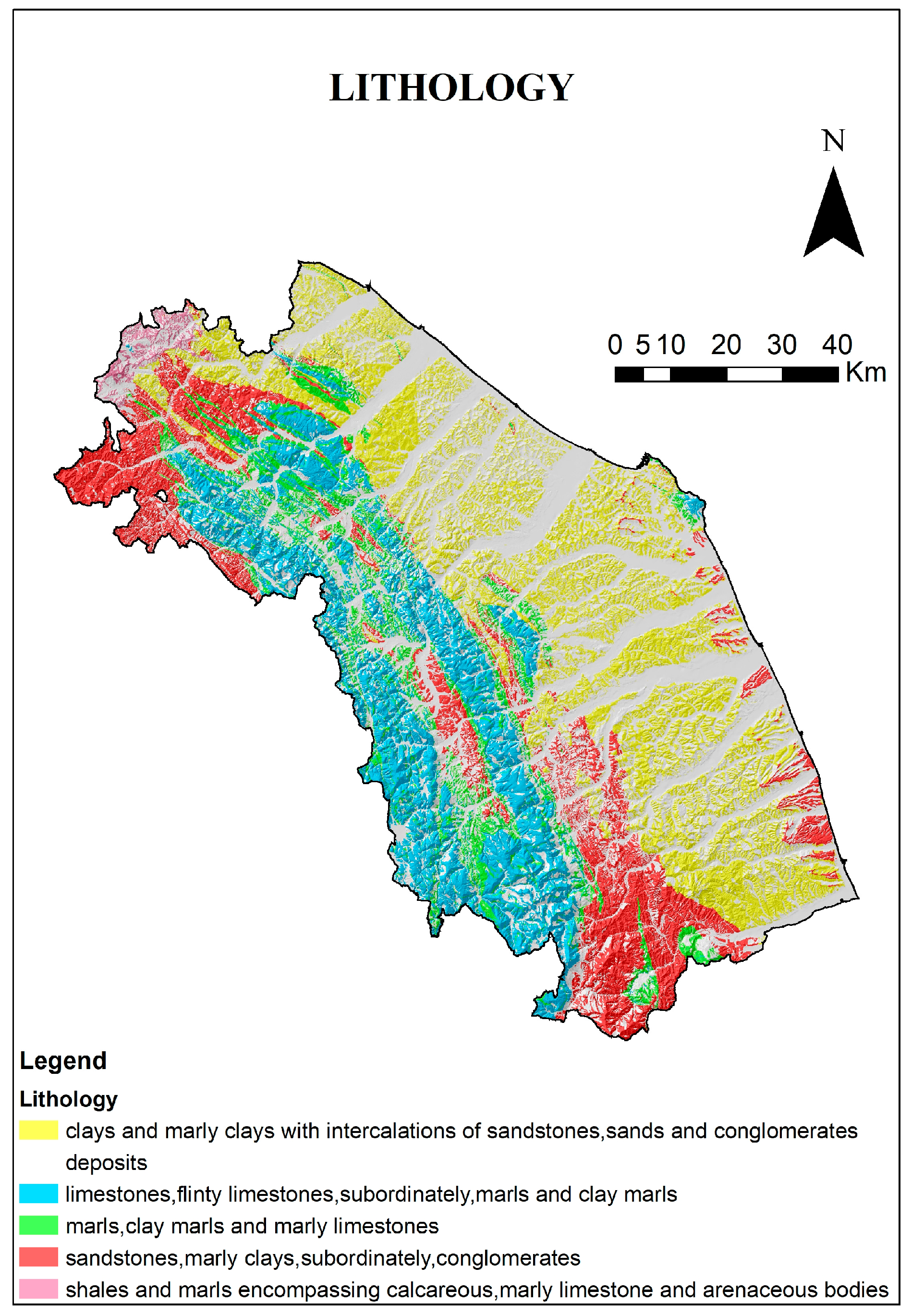
| Geology | |||||
| Clays and marly clays… | Deposits | Limestones, flinty limestones… | Marls, clay marls, and marly limestones | Sandstone, marly clays… | Shales and marls encompassing calcareous |
| Slope | |||||
| 0–5 | 5–15 | 15–25 | >25 | ||
| Exposure | |||||
| Flat | North | East | South | West | |
| Altitude | |||||
| 0–500 | 500–1000 | 1000–2500 | |||
| Causal Factor | TF | TNF | Classes | C | TFoc | TNFoc | Fc | NFc |
|---|---|---|---|---|---|---|---|---|
| Ecological unit | 12.9 | 9351.1 | Airport | / | 12.90 | 9351.04 | 0 | 0.06 |
| Deciduous shrubland | 1.683 | 11.70 | 9172.92 | 1.204 | 178.18 | |||
| Evergreen shrubland | 2.395 | 12.13 | 9297.21 | 0.770 | 53.89 | |||
| Bare area | −1.253 | 12.90 | 9346.78 | 0.002 | 4.32 | |||
| Roads | / | 12.90 | 9350.56 | 0 | 0.54 | |||
| Mixed deciduous woodland | 0.386 | 12.78 | 9292.62 | 0.118 | 58.48 | |||
| Hornbeam woodland | 1.038 | 9.85 | 8326.80 | 3.054 | 1024.30 | |||
| Coniferous woodland | 2.030 | 11.33 | 9181.68 | 1.569 | 169.42 | |||
| Riparian woodland | −0.620 | 12.75 | 9147.31 | 0.150 | 203.79 | |||
| Badland | / | 12.90 | 9345.68 | 0 | 5.42 | |||
| Wood of chestnuts | −1.931 | 12.89 | 9303.16 | 0.010 | 47.94 | |||
| Quarry | / | 12.90 | 9351.03 | 0 | 0.07 | |||
| Arboreal cultivation | −1.070 | 12.78 | 9096.07 | 0.120 | 255.03 | |||
| Continuous built-up area | / | 12.90 | 8862.13 | 0 | 488.97 | |||
| Scattered built-up area | / | 12.90 | 9220.84 | 0 | 130.26 | |||
| Beechwood | −1.791 | 12.85 | 9140.22 | 0.049 | 210.88 | |||
| Herbaceous heter. form. | / | 12.90 | 9346.47 | 0 | 4.63 | |||
| Shores and beaches | / | 12.90 | 9332.71 | 0 | 18.39 | |||
| Arboreal formation | / | 12.90 | 9351.04 | 0 | 0.06 | |||
| Wasteland | 2.924 | 12.89 | 9350.79 | 0.008 | 0.31 | |||
| Lake | / | 12.90 | 9339.17 | 0 | 11.93 | |||
| Holm oak | −3.712 | 12.90 | 9308.26 | 0.001 | 42.84 | |||
| Poplar forest | / | 12.90 | 9351.00 | 0 | 0.10 | |||
| Prairie | −0.310 | 12.35 | 8786.59 | 0.549 | 564.51 | |||
| Pre-forest | 0.866 | 12.82 | 9325.64 | 0.083 | 25.46 | |||
| Decidual oak | 0.981 | 10.34 | 8484.20 | 2.564 | 866.90 | |||
| Seedlet | −0.721 | 10.26 | 4409.03 | 2.644 | 4942.07 | |||
| Aquatic vegetation | / | 12.90 | 9350.78 | 0 | 0.32 | |||
| Psammophilous vegetation | / | 12.90 | 9351.01 | 0 | 0.09 | |||
| Riparian vegetation | / | 12.90 | 9350.92 | 0 | 0.18 | |||
| Urban green | 0.524 | 12.90 | 9349.79 | 0.003 | 1.31 | |||
| TWI | 12.9 | 9351.1 | 0–5 | 0.577 | 8.08 | 7009.21 | 4.82 | 2341.89 |
| 5–10 | −5.340 | 5.47 | 3035.85 | 7.43 | 6315.25 | |||
| 10–15 | −3.900 | 12.29 | 8694.35 | 0.61 | 656.75 | |||
| 15–20 | −3.498 | 12.86 | 9326.79 | 0.04 | 24.31 | |||
| Geology | 12.9 | 9351.1 | Clays and marly clays… | −0.365 | 8.72 | 5005.24 | 4.18 | 4345.86 |
| Deposits | −0.764 | 12.81 | 9293.78 | 0.09 | 57.32 | |||
| Limestones, flinty limestones… | 0.901 | 10.92 | 7574.97 | 1.98 | 1776.13 | |||
| Marls, clay marls, and marly limestones | −0.287 | 11.00 | 8169.25 | 1.90 | 1181.85 | |||
| Sandstone, marly clays… | 0.074 | 12.15 | 8695.95 | 0.75 | 655.15 | |||
| Shales and marls encompassing calcareous | 0.067 | 8.90 | 8029.23 | 4.00 | 1321.87 | |||
| Slope | 12.9 | 9351.1 | 0–5 | −0.601 | 11.12 | 7240.03 | 1.78 | 2111.07 |
| 5–15 | −0.595 | 8.23 | 4612.18 | 4.67 | 4738.92 | |||
| 15–25 | 0.702 | 8.99 | 7696.20 | 3.91 | 1654.90 | |||
| >25 | 0.916 | 10.36 | 8517.84 | 2.54 | 833.26 | |||
| Exposure | 12.9 | 9351.1 | Flat | / | 12.90 | 9346.64 | 0.00 | 4.46 |
| North | −0.245 | 10.00 | 6823.36 | 2.90 | 2527.74 | |||
| East | −0.403 | 10.22 | 6718.84 | 2.68 | 2632.26 | |||
| South | 0.680 | 8.09 | 7189.43 | 4.81 | 2161.67 | |||
| West | −0.131 | 10.40 | 7339.07 | 2.50 | 2012.03 | |||
| Altitude | 12.9 | 9351.1 | 0–500 | −0.644 | 4.58 | 2685.93 | 8.32 | 6665.17 |
| 500–1000 | 0.501 | 8.53 | 7317.15 | 4.37 | 2033.95 | |||
| 1000–2500 | −1.587 | 12.69 | 8712.13 | 0.21 | 638.97 |
Disclaimer/Publisher’s Note: The statements, opinions and data contained in all publications are solely those of the individual author(s) and contributor(s) and not of MDPI and/or the editor(s). MDPI and/or the editor(s) disclaim responsibility for any injury to people or property resulting from any ideas, methods, instructions or products referred to in the content. |
© 2024 by the authors. Licensee MDPI, Basel, Switzerland. This article is an open access article distributed under the terms and conditions of the Creative Commons Attribution (CC BY) license (https://creativecommons.org/licenses/by/4.0/).
Share and Cite
Gentilucci, M.; Barbieri, M.; Younes, H.; Rihab, H.; Pambianchi, G. Analysis of Wildfire Susceptibility by Weight of Evidence, Using Geomorphological and Environmental Factors in the Marche Region, Central Italy. Geosciences 2024, 14, 112. https://doi.org/10.3390/geosciences14050112
Gentilucci M, Barbieri M, Younes H, Rihab H, Pambianchi G. Analysis of Wildfire Susceptibility by Weight of Evidence, Using Geomorphological and Environmental Factors in the Marche Region, Central Italy. Geosciences. 2024; 14(5):112. https://doi.org/10.3390/geosciences14050112
Chicago/Turabian StyleGentilucci, Matteo, Maurizio Barbieri, Hamed Younes, Hadji Rihab, and Gilberto Pambianchi. 2024. "Analysis of Wildfire Susceptibility by Weight of Evidence, Using Geomorphological and Environmental Factors in the Marche Region, Central Italy" Geosciences 14, no. 5: 112. https://doi.org/10.3390/geosciences14050112