Article

Exposure to Selected Geogenic Trace Elements (I, Li, and Sr) from Drinking Water in Denmark

by
Denitza Dimitrova Voutchkova
1,2,*,
Jörg Schullehner
2,3,4,
Nikoline Nygård Knudsen
5,
Lisbeth Flindt Jørgensen
6,
Annette Kjær Ersbøll
5,
Søren Munch Kristiansen
1 and
Birgitte Hansen
2
1
Department of Geoscience, Aarhus University, Høegh-Guldbergs Gade 2, DK-8000 Aarhus C, Denmark
2
Geological Survey of Denmark and Greenland (GEUS), Lyseng Allé 1, DK-8270 Højbjerg, Denmark
3
Department of Public Health, Aarhus University, Bartholins Allé 2, DK-8000 Aarhus C, Denmark
4
Centre for Integrated Register-Based Research at Aarhus University (CIRRAU), Fuglesangs Allé 4, DK-8210 Aarhus V, Denmark
5
National Institute of Public Health, University of Southern Denmark, Øster Farimagsgade 5A, 2nd floor, DK-1353, Copenhagen K, Denmark
6
Geological Survey of Denmark and Greenland (GEUS), Øster Voldgade 10, DK-1350 Copenhagen K, Denmark
*
Author to whom correspondence should be addressed.
Geosciences 2015, 5(1), 45-66; https://doi.org/10.3390/geosciences5010045
Submission received: 29 December 2014 / Revised: 6 February 2015 / Accepted: 16 February 2015 / Published: 27 February 2015
(This article belongs to the Special Issue Medical Geology: Impacts of the Natural Environment on Public Health)

Abstract

:
The naturally occurring geogenic elements iodine (I), lithium (Li), and strontium (Sr) have a beneficial effect on human health. Iodine has an essential role in human metabolism while Li and Sr are used, respectively, as a treatment for various mental disorders and for post-menopausal osteoporosis. The aim here is to evaluate the potential for future epidemiological investigations in Denmark of lifelong and chronic exposure to low doses of these compounds. The drinking water data represents approximately 45% of the annual Danish groundwater abstraction for drinking water purposes, which supplies approximately 2.5 million persons. The spatial patterns were studied using inverse distance weighted interpolation and cluster analysis. The exposed population was estimated based on two datasets: (1) population density in the smallest census unit, the parishes, and (2) geocoded addresses where at least one person is residing. We found significant spatial variation in the exposure for all three elements, related mainly to geochemical processes. This suggests a prospective opportunity for future epidemiological investigation of long-term effects of I, Li, and Sr, either alone or in combinations with other geogenic elements such as Ca, Mg or F.

Graphical Abstract

1. Introduction

Although most chemical elements do not occur exclusively in drinking water (DW), exposures via DW, even at low concentrations, may have important consequences across the entire population [1].
The three trace elements which are in focus here (I, Li, and Sr) have in common that they are essential (I) or possibly essential (Li, Sr) for humans and are currently used as part of pharmaceuticals or dietary supplements. Also, their concentrations in DW can vary spatially, and lifelong exposure to different naturally occurring levels may have an impact on public health in various ways.

1.1. Sources of I, Li, and Sr in Ground- and Drinking Water

Iodine (I) is a trace element from the halogen group and occurs in oxidation states −1, 0, +1, +3, +4, +5, and +7 [2]. However, in the hydrogeochemical cycle, I is found in the stable inorganic forms iodide (I) and iodate (IO3), as well as in various dissolved organic iodine compounds. The speciation data of I in Danish DW reported in [3] showed that there were six speciation combinations. Also, the complex spatial distribution of DW-I was attributed to differences in geological layers, hydrogeochemical reactions, and/or treatment procedures at the waterworks [3]. Iodine concentrations in Danish groundwater are characterised by both small-scale heterogeneity and large-scale spatial trends [4]. Voutchkova et al. [4] found that elevated groundwater-I concentrations originate from Palaeocene and Cretaceous limestone/chalk aquifers, and saw an association between I, Li, Ba, and Br. These elevated concentrations of I in Danish groundwater seemed to be caused by leaching from soil, the marine origin of the aquifers, and/or saline water influence; however, the processes governing the I concentrations were site and depth specific [5].
The lithium (Li) ion at +1 oxidation state is generally soluble and mobile in groundwater; however, sorption onto clay minerals and zeolite occurs [2]. Lithium in groundwater may have multiple geogenic sources. It occurs in the minerals spodumene (LiAlSi2O6) and lepidolite (K2Li3Al4Si7O21(OH,F)3), but also in many other minerals. Pegmatite and brines especially are strongly enriched in Li [6]. In a European study, a median value of 2.6 μg/L Li (min. <0.2 μg/L and max. 75 μg/L) in tap water was found based on 579 samples from all over Europe [2]. To our knowledge, there are no studies focusing on Li sources in Danish groundwater, except for a baseline study, where Hinsby et al. [7] concluded that Li in Miocene aquifers was of natural origin.
Strontium (Sr) occurs in nature in the +2 oxidation state and is the 15th most abundant element on Earth [2]. The size of the Sr2+ ion is intermediate between those of Ca2+ and K+; thus, it substitutes them in many rock-forming minerals [2]. High concentrations of Sr in Danish groundwater were studied by Bonnesen et al. [8], who found that Sr concentrations increased with depth more than would be expected from diffusion of deep connate seawater alone. They concluded that dissolution of small amounts of Sr-rich aragonite (Ca1−xSrxCO3) or equilibrium with the Sr-rich minerals celestite (SrSO4) and strontianite (SrCO3) was the cause of elevated Sr in these chalk formations. Ramsay [9] found a correlation between Mg and Sr, and concluded that recrystallization of Sr-containing aragonite to pure calcite was the main cause of observed elevated Sr concentrations in the chalk aquifers in eastern Denmark. Strontium-enriched groundwater is hence an indicator of limited hydrogeological flushing with fresh water, as carbonate recrystallization takes place on a millennial time scale. Strontium (together with B, Br, Cs, Ge, Li and Rb) is especially enriched in hydrogeochemically mature groundwater [2].

1.2. Public Health and I, Li, and Sr in Drinking Water

Although there are no EU or U.S. standards for I, Li, or Sr, there are national standards for some European countries [2]. A DW standard (maximum values) for I exists in Russia (125 μg/L), for Li in both Russia and Ukraine (30 μg/L), and for Sr in Bosnia and Herzegovina (2 mg/L), Russia (7 mg/L), and Ukraine (7 mg/L) (see references in [2]). The Danish DW standard is 1 mg/L for Li, and 10 mg/L for Sr (provisional), while there is no standard for I [10].

1.2.1. Iodine

Iodine has an essential role in human metabolism [11]. Both insufficient and excessive dietary I intake can cause health problems. Worldwide, the focus is on iodine deficiency (ID), as it is “the single most important preventable cause of brain damage” [12]. Lower IQ, learning capacities, quality of life, and economic productivity are just a few of the adverse effects of severe ID [12]. Even mild ID can result in learning disabilities, poor growth and diffuse goitre in school children [13]. ID is not confined to developing countries [14]: Zimmermann and Andersson [15] estimated that 43.9% (n = 30.5 million) of 6–12-year-old children and 44.2% (n = 393.1 million) of the general population in the World Health Organization (WHO) European Region have insufficient I-intake. Denmark is amongst the 30 countries with ID status worldwide; however, subnational surveys are used for estimating the status in Denmark, as recent nationwide ones are lacking [16].
The recommended daily nutrient intake (RNI) for I is 150 μg for adults (250 μg at pregnancy and lactation), 120 μg for 6–12-year-old children, and 90 μg for babies 0–59 months old [11]. Iodine in the human body originates mainly from food and DW; however, most foods (except sea products) are naturally I low. Therefore, universal salt iodization (USI) programs have been established in many countries, as this is the strategy officially recommended by WHO and United Nations Children’s Fund (UNICEF) for elimination of ID worldwide [11,12]. The sustainability of USI as an ID prevention measure depends on continuous monitoring [12], as well as its integration/coordination with the nationwide strategies for reduction of salt consumption [17]. In the context of the ongoing debate on how to address this issue [14,16,18,19], it is important to focus on regional (local) differences in other I-rich products [18] such as water, milk, etc.
Generally, DW is not considered a major dietary I source, providing only 10% [20]. After the mandatory USI was introduced in Denmark in 2001 [21], about 14% of the dietary I intake was derived from DW and other beverages (w/o juices and milk) [22]. Before the mandatory USI this percentage was 24%–25% [23,24]. It has been shown that local or regional geographical variation of I in DW exists and can be important for the I intake of the population, especially in areas where DW is of groundwater origin, as in Denmark [3,21,25] or China [26,27]. As part of our previous study, the DW contribution to dietary I intake in Denmark was estimated to vary in different parts of the country from 0% to above 100% (adults) or 50% (adolescents) of the RNI [3].

1.2.2. Lithium

Lithium has been used as a treatment for various mental disorders for more than 60 years. The therapeutic doses are much higher than naturally occurring Li levels in DW and typically within a clinical range of 300–1200 mg Li2CO3 per day [28,29]. A substantial amount of studies and meta-analyses investigating patients with mood disorders show that Li significantly reduces suicide mortality in both long-term and short-term treatment [30,31]. It has been hypothesised that if Li in therapeutic doses was effective in preventing suicide in people who already suffer from a mental illness, perhaps Li in small doses over the course of a lifetime could prevent suicide in the general population. This idea has been investigated in several ecological studies on aggregated data. A study from Texas, USA [32] found that counties with high Li levels in DW were associated with significantly lower suicide rates. More recent studies from Japan [33], the U.S. [34], and Austria [35,36]—the latter three also accounting for socioeconomic factors that are closely related to suicide—suggest that long-term intake of small doses of Li via DW may reduce the risk of suicide. Another study in the east of England found no correlation between Li levels in DW and suicide rates [37]. The biochemical mechanisms of action of Li are complex and not fully understood. Studies suggest that Li has a direct antisuicidal effect through a reduction of aggressivity and impulsivity, which are both associated with an increased risk of suicide [38].

1.2.3. Strontium

Osteoporosis is characterised by reduced bone mass and disruption of bone architecture, resulting in increased bone fracture and fragility, and thereby imposing a significant burden on both the individual and society [39]. Hernlund et al. [39] estimated, using a diagnostic criterion from WHO, that approximately 22 million women and 5.5 million men residing in the EU in 2010 had osteoporosis. Of these, approximately 0.28 million were from Denmark (female: 0.22 million, male: 0.06 million) [39,40]. The beneficial effects of stable Sr in the treatment of post-menopausal osteoporosis was reported as early as in the 1950–1960s; however, perhaps because of undue association of the stable naturally occurring isotope with the radioactive Sr isotope, those studies did not receive sufficient attention, and the clinical use of Sr nearly ceased in the 1980s [41]. Currently, therapy for osteoporosis includes dietary supplementation of Ca and Vitamin D, in addition to treatment with oestrogen, pharmaceutical products, or fluoride [42]. Strontium ranelate (Sr2+ and ranelic acid) was licenced and introduced to the European market for treatment of osteoporosis in 2004 [39].
The typical adult body burden of Sr is 0.3–0.4 g (99% in the skeleton), and the primary exposure sources are DW, grains, leafy vegetables, and dairy products [43]. Watts and Howe [43] estimated that the total daily intake of Sr in many parts of the world is up to 4 mg/day, with DW contributing 0.7–2 mg/day (based on 2 L daily consumption of DW with Sr concentrations of 0.34–1.1 mg/L). However, they noted that intakes may be higher in areas where DW concentrations are higher. Watts and Howe [43] and Agency for Toxic Substances and Disease Registry (ATSDR) [44] found that there was not enough evidence for Sr toxicity to humans and that human data were inadequate for setting a tolerable intake and a tolerable concentration of Sr.
The positive effects of Sr supplementation on bone have been examined in rats, monkeys, laying hens, and humans in various studies (a few examples are given in [41,42,45]). Very few studies of lifelong Sr exposure effects exist, as reviewed by ATSDR [44]. Dawson et al. [46] measured Sr in DW and urine (n = 2187) in families that had been residing within their respective communities for at least 10 years, and found a statistically significant product-moment correlation for decreased community mortality rate (in people over 45 years old) for hypertension with heart disease. Polyakova [47] proposed a classification dividing the Arkhangelsk region (Russia) into three zones with different probabilities of Kashin-Beck or similar bone disease manifestation based on the hypothesis that areas with DW characterised by Ca/Sr < 100 are coinciding with Kashin-Beck endemic regions. Curzon [48] found an association between caries prevalence and Sr in DW for lifelong residents in four Ohio cities, with minimum caries prevalence at DW concentrations around 5–6 mg Sr/L. There are few indications that Sr, likely in combination with other trace elements, such as F or Ba, could be beneficial to enhancing remineralisation of teeth, and hence protection against caries (for more references see [49]). To our best knowledge, there are no published reports on the potential public health effects (beneficial or adverse) of long-term exposure to different levels of naturally occurring Sr in DW in combination with Ca, F, or other DW constituents.

1.3. Study Objectives

The general objective of this study is to evaluate the potential for future epidemiological investigations of long-term (lifelong, chronic) exposure to low doses of three naturally occurring compounds (I, Li, and Sr) from DW. The specific study aims are accordingly (1) to characterise the nationwide spatial patterns of I, Li, and Sr concentrations in Danish DW and (2) to quantify the exposure to I, Li, and Sr from Danish DW.

2. Experimental Section

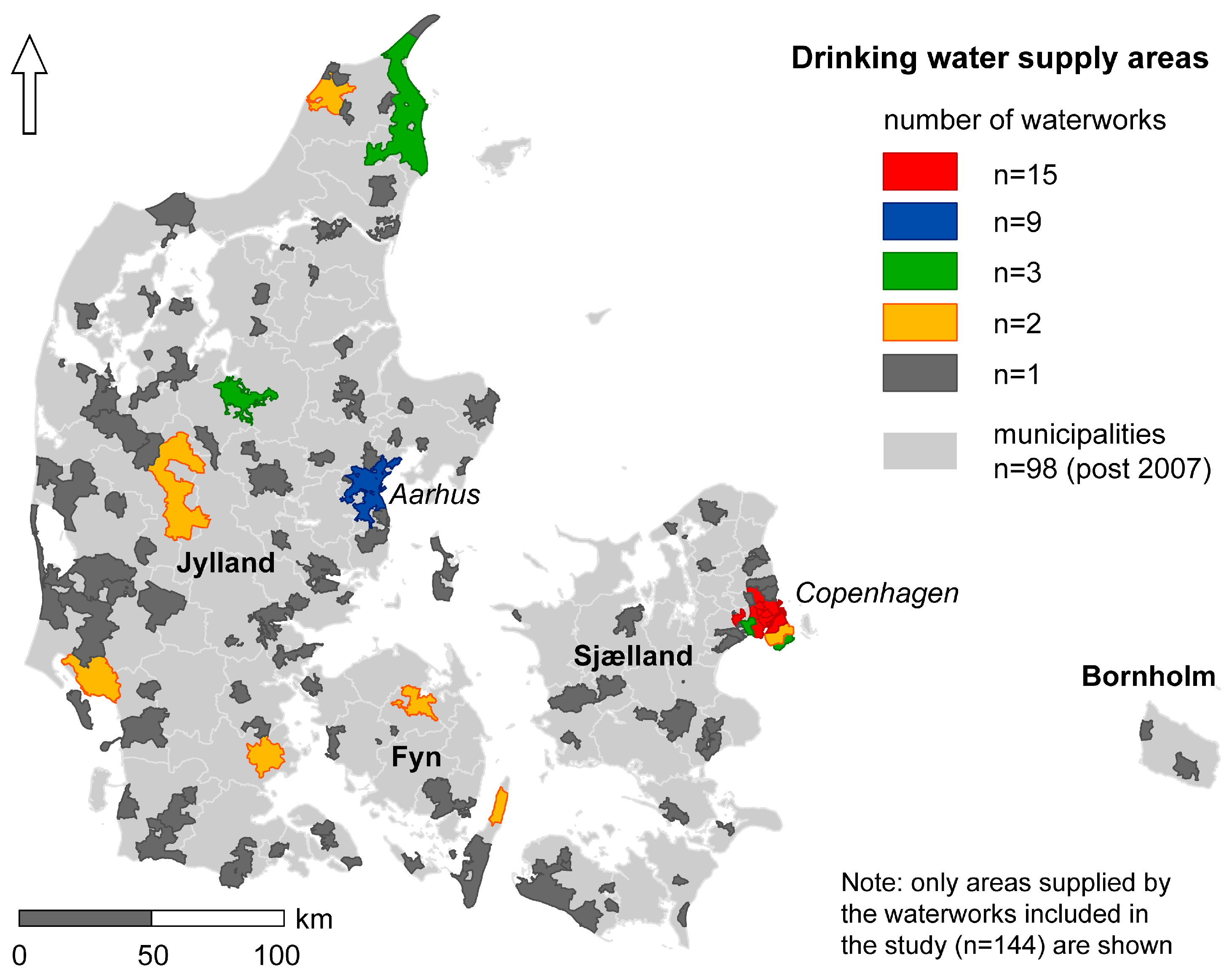
2.1. Danish Public Drinking Water Supply

Denmark is a relatively small country (approximately 43,000 km2) with about 5.6 million inhabitants. The Danish DW supply is entirely of groundwater origin. The major part of the population is supplied by public waterworks. The reported groundwater abstraction for DW purposes for 2010 was 397 million m3 (by 2585 public waterworks) [50]. Next to the public waterworks, there are single wells and small waterworks (supplying <10 households), which were estimated to supply about 0.4 million people (7%) [51].
The DW supply is highly decentralised. Sørensen and Møller [52] reported that about 72% of the active waterworks have annual abstractions of <0.1 million m3, whereas only about 3% are abstracting >1 million m3.
Bottled water consumption in Denmark was amongst the lowest in Europe in 2013 (22.8 L/cap or 0.127 million m3 [53]) and below the global average (30 L/cap [54]). Thus, the major source of potable water in Denmark is delivered by public waterworks.
Generally, Danish groundwater requires simple treatment with aeration and sand filtration only. In the aeration step, naturally occurring gasses such as methane are removed and substituted by oxygen. During filtration, oxidised iron and manganese are removed. A few other components are detained in the sand filters in various magnitudes. Only 74 waterworks, producing about 50.47 million m3, use some sort of more advanced water treatment [55]. However, neither chlorination nor ozone treatment was used in Denmark by 2012 [55].
The aquifers used for DW abstraction in Denmark are mainly unconsolidated Quaternary glacial sand, Tertiary marine and fluvial sand or Cretaceous limestone and chalk.

2.2. Water Chemistry Data (I, Li, and Sr)

The chemical data used here is from a DW sampling campaign conducted from April to June 2013 and reported in detail in [3,56]. The samples represent treated DW from groundwater origin, ready to be supplied to consumers (sampling point: exit waterworks). The treatment consists of aeration and sand filtration, except for 10.4% (n = 15) of the 144 waterworks, where a somewhat more advanced water treatment method is used [3].
Iodine data were collected for all of the waterworks included in the study (n = 144); however, where there were no total I measurements (n = 5), iodide (I) determined by Ion-exchange chromatography (IC) was used instead. Lithium and Sr data were obtained for 139 of the locations. The 144 waterworks abstract about 175 million m3 annually, which accounts for 45% of the total groundwater abstraction by all public water supplies (excluding small waterworks or wells supplying fewer than 10 households) [3]. The samples were filtered in the lab (0.45 μm pore size Q-max syringe filter, Frisenette Aps, Ebeltoft, Denmark). Inductively coupled plasma mass spectrometry (ICP-MS) was used for determining I, Li, and Sr concentrations. A short summary of I, Li, and Sr data is presented in Table 1. Further details on the laboratory methods, sampling design and execution, hydrogeochemical characterisation, and water treatment are provided in [3,56].

2.3. Water Supply Areas

Schullehner and Hansen [57] recently compiled a map with the water supply areas of all 2852 public waterworks in Denmark but excluding a number of very small waterworks and wells supplying <10 households. For the purposes of our study, we have used only the areas supplied by the 144 included waterworks (Figure 1). It should be noted that: some of the selected areas are supplied by more than one waterworks (Figure 1) and it is possible that some of the residents in these areas are not connected to the public water supply but get their water from a privately owned well [57].
Table 1. Summary of the iodine, lithium, and strontium datasets (concentrations in drinking water) used in this study.
TitleIodine (I)Lithium (Li)Strontium (Sr)
Unitμg/Lμg/Lmg/L
Lab methodICP-MS *ICP-MSICP-MS
Count (n)144 *139139
Detection limit (d.l.)0.250.005
<d.l. (%)6.2518.70
Substitution (0.5*d.l.)0.12.5-
Min. concentration0.12.50.07
Max. concentration12630.714.45
Mean concentration13.97 *11.041.31
Median concentration11.25 *10.300.59
Notes: * Here I was used where total iodine was not measured (n = 5); IC is the method for I; because these I measurements are included, the mean and median calculated here differ slightly from [3].
Figure 1. Water supply areas of the waterworks included in the study (n = 144); the areas in red, blue, green, and orange are supplied by more than one of the included waterworks (source: map on supply areas of 2852 Danish waterworks [57]).
Geosciences 05 00045 g001
All selected water supply areas were assigned the water quality measurements (I, Li, and Sr) of the waterworks by which they are supplied. The areas supplied by more than one waterworks were assigned the average concentrations measured at the waterworks supplying the specific area (Figure 1). The two largest cities, Copenhagen and Aarhus, are supplied with water treated by at least 15 and nine waterworks, respectively. An effort was made to pinpoint specific parts of the cities (neighbourhoods), which are preferentially supplied with water from one/some of these waterworks. Previously collected data from the water supply companies (as part of two studies [3,57]) was used for this purpose. However, for parts of the cities (blue and red areas from Figure 1) this was not possible, as the water from all these waterworks is mixed together in the water distribution system. More precise estimations of I, Li, and Sr concentrations are possible only if water samples are obtained at carefully selected points in the distribution system, which was not feasible for this study.

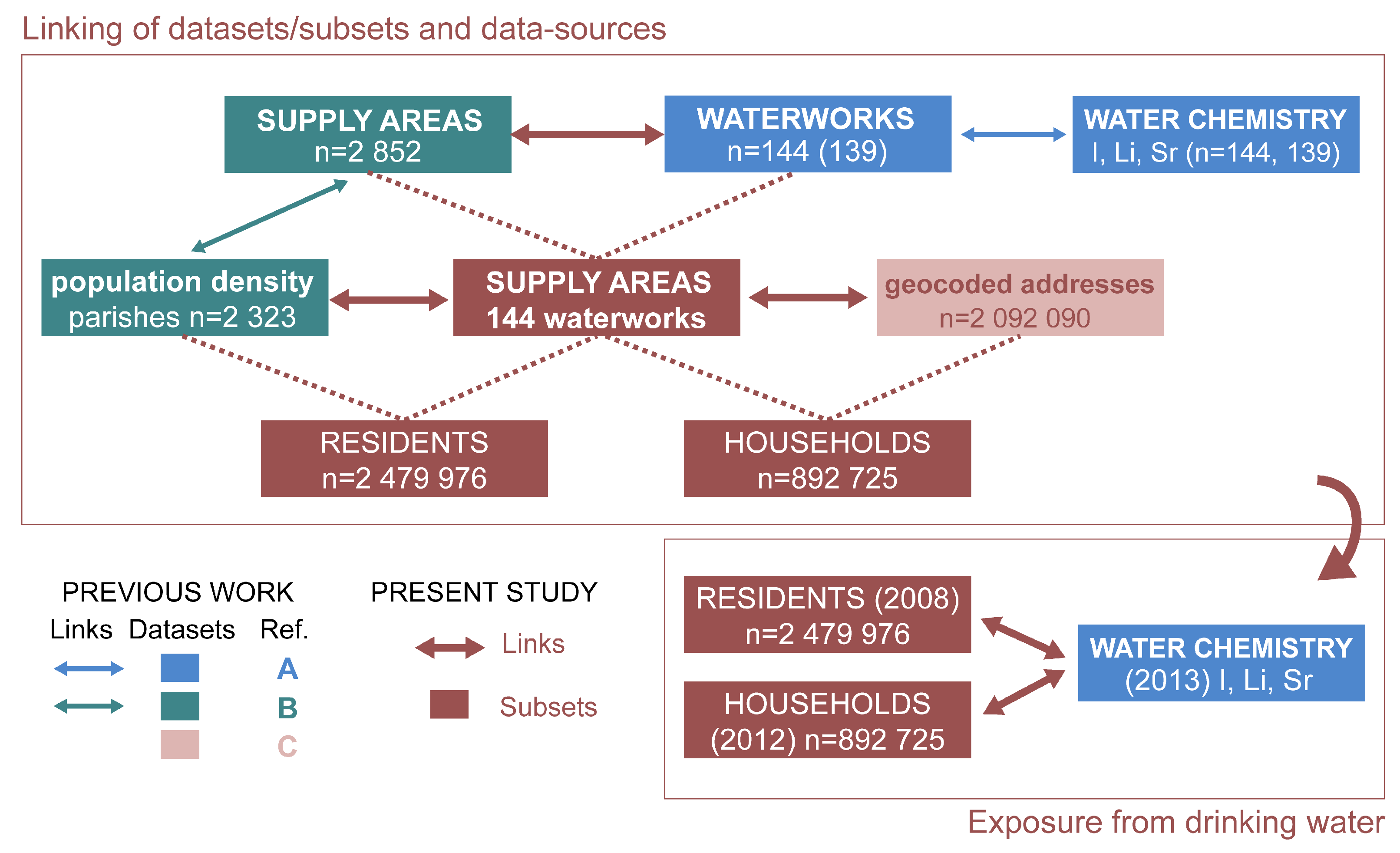
2.4. Estimation of the Population Living in the Selected Water Supply Areas

Two datasets were used for estimating the population living in the selected areas:
  • 1st dataset: a population density map based on the population counts in the smallest census unit (parishes) for 2008 (further details can be found in [57]). This method yields “number of residents” in the selected supply areas.
  • 2nd dataset: a database including geocoded addresses with at least one registered resident from the Danish Civil Registration System (DCRS), provided by the Centre for Integrated Register-Based Research at Aarhus University (CIRRAU). This database contains one record for each specific address (municipality, road, house number, and, if relevant, door number) used as a residence in DCRS [58]. The DCRS was established in 1968 and has since recorded current and historical information not only on the place of residence, but also on vital status, gender, place and date of birth, parents, spouses, and siblings and twins for all persons living in Denmark [59]. This information is regarded as being of very high quality and yields an important and rare asset which can be used for epidemiological research [59]. A subset of this database has been used here. It consists of the geocoded addresses for 2012 only (n = 2,092,090), which are further referred to as “households”.
The number of residents (1st dataset) and the number of household addresses (2nd dataset) within each water supply area were calculated using the geographical information system ArcMap 10.0 (Esri, Redlands, CA, USA).

2.5. Inverse Distance Weighted Interpolation and Cluster Analysis

2.5.1. Data Pretreatment

Due to skewed distributions of I and Sr concentrations, a square root transformation of I and a logarithmic transformation of Sr were applied prior to analysis. The transformations were selected by comparing the distribution of the transformed measurements with a normal distribution.

2.5.2. Inverse distance weighted interpolation

Inverse distance weighting (IDW) was used to estimate a density surface for each of the elements I, Li, and Sr. This method assigns a weighted average of the neighbouring values to each unmeasured grid cell on the map. The weight given to each observation is a function of the distance between that observation’s location s i and the grid point s 0 at which the interpolation is desired. Generally, the inverse distance interpolator is given as in Equation (1):
Z ^ ( s 0 ) = i = 1 n ω ( s i ) Z ( s i ) i = 1 n ω ( s i )
where Z ^ ( s 0 ) is the predicted value at the unsampled location s 0 and Z ( s i ) is the observed value at the ith location within a given maximum distance for i = 1, …, n, with n being the number of locations in the study. The weights ω attributed to the observations were computed as in Equation (2):
ω ( s i ) = | | s i s 0 | | p
where | | s i s 0 | | is the Euclidian distance between locations s 0 and s i and p is an inverse distance weighting power. The weighting power is selected in order to determine how fast the weights tend towards zero as the distance from the grid point increases [60,61,62].
Grid cells of 1 × 1 km, a power of p = 2, and a maximum distance of 75 km were applied. The density maps of I and Sr were derived using a square root and a logarithm transformation, respectively. Back-transformed interpolated values were calculated and mapped.

2.5.3. Cluster Analysis

A local cluster analysis was performed to investigate areas with significantly higher or lower levels of I, Li, or Sr in the DW. I and Sr were transformed prior to the analysis. The presence, significance, and approximate location of clusters were evaluated using spatial scan statistics implemented by Kulldorff [63] in the software SaTScan (v9.3.1, http://www.satscan.org/). The spatial scan statistic searches for clusters by using a search window of varying shape and size. For each location, a test is performed, evaluating whether the mean value is significantly higher (or lower) within the search window compared to outside. Given the continuous data, a normal distribution was used as the probability model in which the null hypothesis was that all observations come from the same distribution, whereas the alternative hypothesis was that there was one cluster location where the measurements have either a larger or smaller mean than outside that cluster. A central feature of this method is that the statistical inference is still valid, even if the true distribution is not normal [64].
The significance of identified clusters was tested using a likelihood ratio test with a p-value obtained using Monte Carlo simulations (999 permutations). The likelihood function is maximized over all window locations and sizes, and the one with the maximum likelihood constitutes the most likely cluster. An elliptic search window with a centre at the location of each waterworks was used, allowing no geographical overlap between clusters. The maximum percentage of the measurements to be included in a cluster was varied at 10%, 20%, 25%, 30%, and 50%, respectively. Changing the maximum percentage of the measurements included in a cluster did not change the location and number of clusters identified. A maximum percentage of 20% of the measurements included in a cluster was used.

2.6. Exposure Analysis

To estimate the exposure to I, Li, and Sr from DW the following data were used: (1) water chemistry data, which was assigned to each of the supply areas and (2) the 1st and 2nd datasets with the number of residents and the number of households in the selected supply areas, respectively. A schematic visualisation of the different datasets (and subsets) and the links between them is provided in Figure 2.
Figure 2. Scheme presenting the datasets, their subsets, and the links between them used in this study. Some of these datasets and links were prepared in previous studies (colour coded, references: A [3], B [57], and C [58]).
Geosciences 05 00045 g002
It was estimated that 2,479,976 residents (about 45.3% of all residents in 2008) and 892,725 households (42.7% of all households in 2012) are supplied with DW by the 144 waterworks analysed in this study. For the 139 waterworks where Li and Sr data are present, the number of residents is 2,442,705 (about 44.6%) and the number of households is 874,375 (41.8%). Thus, the exposure analysis covers close to half the population of Denmark (see Figure 1 for spatial reference).
The calculation of residents and households exposed to different levels of I, Li, and Sr are given as a percentage of the households and population included in this study, respectively.

3. Results and Discussion

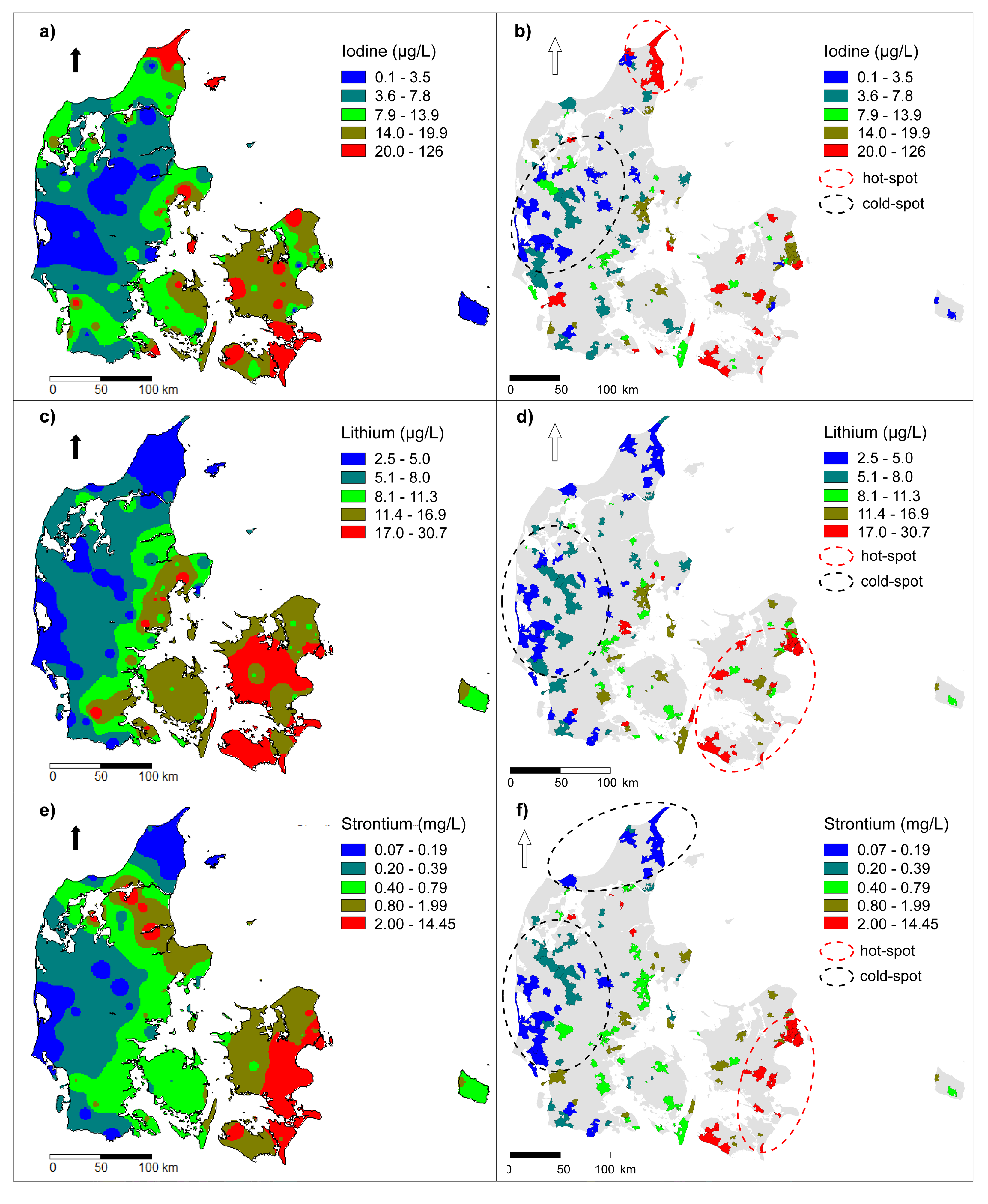
3.1. Spatial Distribution of Drinking Water I, Li and Sr

The spatial distribution of I, Li, and Sr concentrations in treated DW of groundwater origin was examined using IDW interpolation and cluster analysis. The IDW interpolated maps are presented in Figure 3a,c,e. The cluster analysis identified areas with significantly high concentrations and significantly low concentrations of each of the elements I, Li, and Sr. The number of measurements (i.e., waterworks) in a cluster, mean concentrations inside and outside the clusters, and p-values for the three elements are shown in Table 2. The ellipses of the significant hot and cold spots are presented overlaying the maps with the supply areas (see Figure 3b,d,f). However, it should be kept in mind that the cluster analyses are based on point data.
The lowest concentrations for all three elements are observed in the western part of Jylland, where the significant cold spots of I, Li, and Sr also are located. Another similarity in the spatial patterns is the general east-west trend: relatively higher concentrations are found in the eastern part and lower in the western part of the country. Despite that, the spatial distribution of I, Li, and Sr also show differences.
Figure 3. Iodine, lithium, and strontium in drinking water in Denmark; (a,c,e) IDW interpolation; (b,d,f) drinking water concentrations in the selected supply areas and hot and cold spot clusters. Note: each category represents ~20% of the observations; the cluster analysis is based on the point data. See Section 2 for details.
Geosciences 05 00045 g003
An east-west trend for I concentrations in DW was reported by [25,65] and is thereafter largely used by others. However, based on a cluster analysis of I data characterised by higher spatial sampling resolution, Voutchkova et al. [3] concluded that there is complex spatial variation and the east-west trend is an oversimplification. The same data as in [3] are used in the current study, while the different analyses employed here add to our previous work; e.g., the IDW interpolated maps (Figure 3a) visually confirm our statement about the complexity of the spatial variation. Northern Jylland is found to be a significant hot spot of DW-I by both the present and the previous analysis [3]. However, due to different data pretreatment (here: square root transformation vs. normal score transformation in [3]) and analytical method (here: spatial scan statistics vs. Local Moran’s I in [3]), a second hot spot (Sjælland according to [3]) was not found here. The governing factors for this complex spatial pattern have been attributed to both the geology and the groundwater treatment procedures [3].
Table 2. Geographical clusters of high (hot spot) and low concentrations (cold spot) of iodine, lithium, and strontium in drinking water.
ElementType of ClusterNmeasurements Inside ClusterMean Concentrationp-value
Inside ClusterOutside Cluster
Iodine (μg/L)Hot spot477.099.920.001
Cold spot262.3713.690.003
Lithium (μg/L)Hot spot2719.089.100.001
Cold spot274.5621.600.002
Strontium (mg/L)Hot spot272.660.450.001
Cold spot270.210.840.001
Cold spot100.150.720.049
Of all three elements, Li is the one with the most clearly manifested east-west trend: a smooth transition between the low (Li < 8 μg/L) and the high concentrations (Li > 17 μg/L) is characteristic. A significant hotspot is covers parts of Sjælland and the islands to the south (Figure 3c).
The highest Sr concentrations (>2 mg/L) are observed in the eastern part of Sjælland (covered by the significant hot spot, too), as well as in a few locations in Jylland. The hot spot for Sr is slightly smaller than the one for Li. Strontium is also the only element from the three which has a second significant cold spot, located on the raised Holocene seabed in northern Jylland.

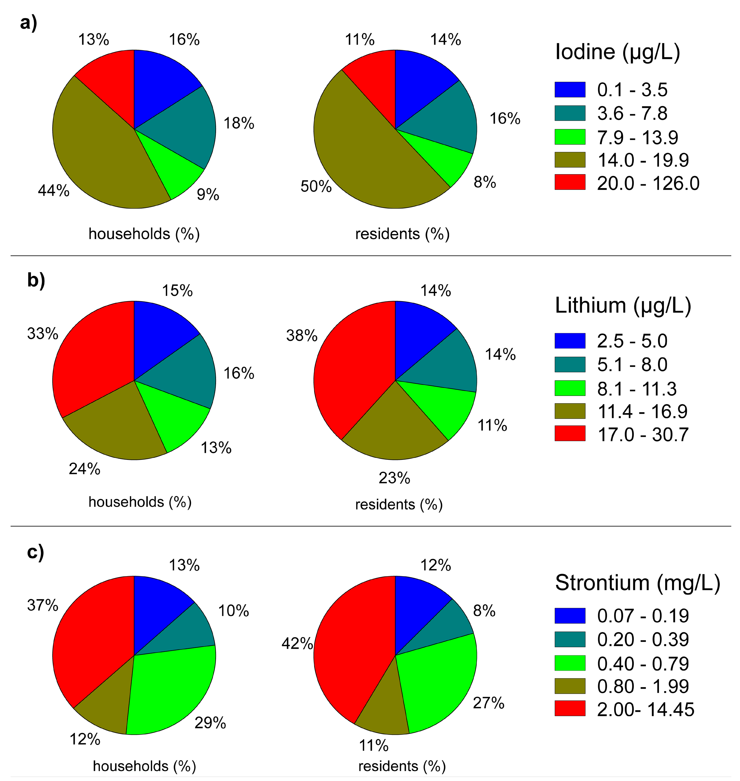
3.2. Exposure to I, Li, and Sr via Drinking Water

The exposure to different concentrations of I, Li, and Sr from treated DW (groundwater origin) is given as percentage of exposed consumers or households from the ones included in this study, i.e., the residents and households within each water supply area where I, Li, and Sr measurements were available (Figure 4; see Table 3 for absolute numbers).
The largest proportion of households (h) and residents (r) in this study are exposed to I concentrations in the range of 14–20 μg/L (h: 44%, r: 50%), Li concentrations in the highest range of 17–30.7 μg/L (h: 33%, r: 38%), and Sr concentrations in the range of 2–14 mg/L (h: 37%, r: 42%). However, only a small proportion of the population is exposed to the highest levels of the observed concentrations: 0.8% (h) or 0.4% (r) are exposed to Sr > 10 mg/L, which is the current provisional DW standard in Denmark; 1.7% (h) or 1.8% (r) are exposed to Li > 25 μg/L; and 0.5% (h) or 0.6% (r) are exposed to I > 50 μg/L. This exposure calculation takes into account the population density for 2008 (r) or all geocoded residential addresses in 2012 (h) in the areas supplied by the selected waterworks. Thus, it provides information on the differences in exposure based on the spatial variation of I, Li, and Sr in DW. The spatial distribution of DW supply areas exposed to different levels of I, Li, and Sr is provided in Figure 3b,d,f. From the results presented in Figure 4 (and Table 2), it can be concluded that there is a contrast in the exposure of the Danish population to I, Li, and Sr from DW. Possible health effects of these exposure contrasts could be studied by combining these results with data from the Danish health registers [66].
Figure 4. Proportion of households and residents exposed to different concentrations of (a) iodine, (b) lithium, and (c) strontium. Note: the number of households and number of residents are estimated using two different datasets (see Section 2); see Table 3 for absolute numbers.
Geosciences 05 00045 g004
Table 3. Households and residents exposed to different concentrations of iodine, lithium, and strontium in absolute numbers (n) and in percentages (%; see also Figure 4).
ElementConcentrationHouseholdsResidents
n%n%
Iodine<3.6 μg/L140,59315.7356,53314.4
3.6 to 7.8 μg/L158,21317.7388,00815.6
7.9 to 13.9 μg/L80,6779.0201,4788.1
14.0 to 19.9 μg/L396,07044.41,250,45750.4
20.0 to 126.0 μg/L117,17213.1283,50011.4
Total892,7251002,479,976100
Lithium<5.1 μg/L130,95415.0332,61313.6
5.1 to 8.0 μg/L138,44115.8335,87513.8
8.1 to 11.3 μg/L109,87912.6277,07811.3
11.4 to 16.9 μg/L207,90723.8556,75922.8
17.0 to 30.7 μg/L287,19432.8940,38038.5
Total874,3751002,442,705100
Strontium<0.2 mg/L116,28413.3300,85612.3
0.20 to 0.39 mg/L84,1459.6199,1148.2
0.40 to 0.79 mg/L250,70528.7654,18326.8
0.80 to 1.99 mg/L103,08711.8272,12811.1
2.00 to 14.45 mg/L320,15436.61,016,42441.6
Total874,3751002,442,705100

3.3. Discussion

The spatial variation of I concentrations in Danish groundwater is characterised both by a large-scale east-west trend [4] and by small-scale variation [4,5]. This is also clearly reflected in the geographical trend of the treated DW-I, which was shown here and in [3]. The elevated I concentrations in Danish DW and groundwater were found to be associated mainly with the Palaeocene to Cretaceous limestone or chalk and postglacial marine-sand aquifers [3,4,5].
There is limited information about the Li content in Quaternary and Tertiary deposits [7], and especially about the geochemical processes governing the release of Li to groundwater. Lithium is strongly enriched in ocean water compared to freshwater, and in brines. This may lead to the hypothesis that Danish aquifers of marine origin are Li enriched compared to those of glacial and fluvial origin. Moreover, an association between I and Li pointing at saline water influence was found based on Danish historical groundwater data [4].
Strontium concentrations in Danish DW seem to be similar to average concentrations in U.S. streams (between 0.5 and 1.5 mg/L) but higher than average Sr concentrations in U.S. groundwater (<0.5 mg/L) as reported by ATSDR [44]. The hot-spot location supports the regional findings by Ramsay [9] that local differences in the pre-Quaternary chalk and limestone aquifer geology and hydrogeology are responsible for elevated Sr concentrations in present-day groundwater. However, the lower Sr concentrations in DW (western part of Denmark) are most probably governed by the relatively constant contributions from the weathering of Sr-poor silicates in the soil, which is strongly dependent on texture and mineralogy, and from the dissolution of Sr-poor carbonates at the acidification front.
The significant spatial difference in the concentrations of I, Li, and Sr in Danish DW results in varying human exposure to these elements. Therefore, there is great potential for future epidemiological investigations of the long-term (lifelong, chronic) exposure to low doses of the three selected naturally occurring compounds from DW. In addition to exposure to a single element, there is a potential for studying the effects related to a combination of these and additional elements.
For example, in a project from Norway, nationwide data on municipal DW was combined with data on all registered treated hip fractures to study whether Ca and Mg have a protective function [67]. Corresponding studies based on Sr in a single exposure or in combination with Ca, Mg, or F in Danish DW, residential history and the various nationwide registers on health and social issues [66] can be conducted. The spatial distribution of Sr in Danish DW resembles somewhat the spatial distribution of F [68] and Ca and Mg [69]. Hence, this first prospective data analysis reveals a large potential for future nationwide public health studies, especially if Sr in DW is combined with Ca, Mg, and F. Findings relating Sr in DW to life-long health, as reported by Curzon [48] and Dawson et al. [46] on hypertension and caries, could most likely be improved considerably with such a multi-element approach, as Sr is closely related to Ca incorporation in human bones [42].
Similarly, an epidemiological investigation can elucidate whether the observed spatial differentiation in exposure to I from DW (see also [3]) influences the health status of the Danish population. The DCRS yields the unique possibility to connect past exposure of mothers (e.g., during pregnancy) to I from DW with the health status of their children in order to explore, whether the observed spatial differences in DW-I affect the children’s performance (e.g., physical and mental development).
With respect to Li, there is currently an ongoing nationwide study conducted at the National Institute of Public Health (University of Southern Denmark, Copenhagen, Denmark) using geospatial methods to investigate whether long-term intake of naturally occurring low doses of Li in DW is protective against suicide, when accounting for socioeconomic as well as other factors.
The presented exposure analysis is based on water chemistry data from a single point in time. There is only limited data on the temporal variability of the studied geogenic elements in both treated DW and groundwater in Denmark. A comparison between the Li data used here and other, previously unreported Li measurements can be seen in Figure 5a, showing that the Li levels are similar even though the analytical methods (ICP-MS vs. Atomic absorption spectroscopy (AAS)) and the sampling dates differ (2013 vs. 2009–2010).
Figure 5. (a) Lithium concentrations in untreated mixed groundwater from well sites (black dots) at seven waterworks in the Copenhagen area and in treated drinking water (data from two studies are used: a the ICP-MS data reported here and in [3] (red +), b unreported AAS data provided by the waterworks (blue +; see Supplementary materials for further detail). (b) Comparison between I concentrations in drinking water (red +) and untreated groundwater from wells (black dots) of five waterworks located in Jylland (c data from 2012 reported in [70]).
Geosciences 05 00045 g005
These results imply that the Li concentration in DW at the given waterworks can be assumed to be stable over time. Another interesting aspect is that most of the large waterworks extract water from many wells, often grouped in well sites. As there are differences in I, Li, and Sr concentrations in the abstracted groundwater (Figure 5a, black dots), abstraction volumes and pumping strategies will govern the resulting concentrations in the treated DW. An illustration of the differences in Li concentrations in mixed groundwater at/between the well sites of seven waterworks in the Copenhagen area and the Li concentrations in treated DW at these waterworks is also presented in Figure 5a. Further, the results imply that there is no Li removal or enrichment during the treatment. A similar comparison between groundwater and treated DW is made for I at five waterworks located in Jylland (Figure 5b) based on the 2012 data reported in [70]. This comparison implies that at least at some waterworks, I can be partially removed by treatment (DW-I is lower than the groundwater-I concentrations). The issue of the effect of treatment and the temporal variation of the I concentrations in DW is further discussed in [3]. To our best knowledge, no such analysis exists on Sr in Danish DW or groundwater.
Another limitation of this exposure analysis (or future epidemiological studies based on these data) is that some misclassification could have occurred, as some of the households/residents included here may be supplied by private wells. There is also uncertainty associated with the concentrations in the supply areas where more than one waterworks distributes DW to the consumers (see Figure 1). Yet another issue is connected to the fact that we used I, Li, and Sr concentrations in DW at the exit of the waterworks but not much is known about whether these elements are involved in chemical processes in the distribution system before the DW reaches the consumer. Further investigations are needed in order to evaluate the effect of these misclassifications and/or uncertainties.
Last but not least, some limitations with respect to the exposure levels are due to the data on geographical location of the residency addresses. For the purposes of carrying out an epidemiological study on possible health effects, it is important to take the residential history of each studied individual into account. This is possible using the DCRS database. However, the exposure estimation will still be associated with uncertainty due to e.g., individuals commuting to areas with different exposure characteristics. Data from Statistics Denmark for 2013 shows that 470,950 people or about 31% of the employed Danish population commute less than 5 km, whereas about 7.6% commute more than 50 km (202,289 people).

4. Conclusions

This study revealed significant spatial variations in I, Li, and Sr concentrations in Danish DW representing approximately 45% of the annual groundwater abstraction for DW purposes. A general east-west trend of relatively high concentrations in the eastern part and lower ones in the western part of the country was observed. However, there are element-specific smaller-scale differences, so the general trend should be interpreted cautiously. The exposure to different I (Li, Sr) levels covers about 45.3% (44.6%) of all residents (2008) and 42.7% (41.8%) of all households (2012) that were supplied with DW by the investigated waterworks (I: 144; Sr and Li: 139). The spatial distribution of I, Li, and Sr in DW results in an exposure contrast of these elements. The largest part of the population (about 40%) is exposed to 14–20 μg I/L, 17–30.7 μg Li/L, and 2–14 mg Sr/L. The rest of the population covered here is exposed to both higher and lower I concentrations from DW. For Li and Sr, this range is at the upper end of the observed concentrations; thus the rest of the population is exposed only to lower Li and Sr concentrations in DW. The results presented here show that there is a great potential for future epidemiological studies on the long-term (lifelong, chronic) effects of exposure to I, Li, and Sr from DW as single elements. Additionally, it is also possible to include other relevant elements.

Acknowledgments

We would like to thank Malene Thygesen and the Centre for Integrated Register-Based Research at Aarhus University (CIRRAU) for the provision of the geocoded Danish addresses, and, Ann-Katrin Pedersen from HOFOR (The Greater Copenhagen Water Supply Company) for performing the AAS data analyses on lithium (Figure 5a and Supplementary materials), and providing these data for the present study. The rest of the water chemistry data as well as some of the data on supply areas was collected as part of a GEOCENTER (Denmark) project (2011–2014) funded by the Geological Survey of Denmark and Greenland (GEUS) and Aarhus University (Denmark). The authors express their sincere gratitude to the rest of the GEOCENTER project participants.

Author Contributions

The linking of the different data sources and the exposure analyses was done by D.D.V. and J.S. The IDW and the cluster analyses were performed by N.N.K. and A.K.E. The data for Figure 5 on Li in the groundwater and drinking water, as well as interpretation was provided by L.F.J. B.H. and S.M.K. provided background information and supervised the project. D.D.V compiled the initial version of this manuscript, with all authors contributing by writing different sections of it. All authors have equally participated in the revisions and the final editing of this text prior to its submission.

Supplementary Materials

Supplementary materials which include additional information on the unpublished data from Figure 5a can be accessed at: https://www.mdpi.com/2076-3263/5/1/45/s1.

Conflicts of Interest

The authors declare no conflict of interest.

References and Notes

  1. Villanueva, C.M.; Kogevinas, M.; Cordier, S.; Templeton, M.R.; Vermeulen, R.; Nuckols, J.R.; Nieuwenhuijsen, M.J.; Levallois, P. Assessing exposure and health consequences of chemicals in drinking water: Current state of knowledge and research needs. Environ. Health Perspect. 2014, 122, 213–221. [Google Scholar] [PubMed]
  2. Reimann, C.; Birke, M. Geochemistry of European Bottled Water; Borntraeger Science Publishers: Stuttgart, Germany, 2010. [Google Scholar]
  3. Voutchkova, D.D.; Ernstsen, V.; Hansen, B.; Sørensen, B.L.; Zhang, C.; Kristiansen, S.M. Assessment of spatial variation in drinking water iodine and its implications for dietary intake: A new conceptual model for Denmark. Sci. Total Environ. 2014, 493, 432–444. [Google Scholar] [CrossRef] [PubMed]
  4. Voutchkova, D.D.; Kristiansen, S.M.; Hansen, B.; Ernstsen, V.; Sørensen, B.L.; Esbensen, K.H. Iodine concentrations in Danish groundwater: Historical data assessment 1933–2011. Environ. Geochem. Health 2014, 36, 1151–1164. [Google Scholar] [CrossRef] [PubMed]
  5. Voutchkova, D.D.; Hansen, B.; Ernstsen, V.; Kristiansen, S.M. Hydro-geochemical characterisation of Danish groundwaters in relation to iodine. Paper III in PhD thesis [70].
  6. Kesler, S.E.; Gruber, P.W.; Medina, P.A.; Keoleian, G.A.; Everson, M.P.; Wallington, T.J. Global lithium resources: Relative importance of pegmatite, brine and other deposits. Ore Geol. Rev. 2012, 48, 55–69. [Google Scholar] [CrossRef]
  7. Hinsby, K.; Rasmussen, E.S.; Henriksen, H.J. European Reference Aquifers: The Miocene Sand Aquifers of Western Denmark. In Report for the EU Research Project (‘BASELINE’): Natural Baseline Quality of European Groundwater: A basis for Aquifer Management; Geological Survey of Denmark and Greenland (GEUS): Copenhagen, Denmark, 2003; pp. 1–18. [Google Scholar]
  8. Bonnesen, E.P.; Larsen, F.; Sonnenborg, T.O.; Klitten, K.; Stemmerik, L. Deep saltwater in Chalk of North-West Europe: Origin, interface characteristics and development over geological time. Hydrogeol. J. 2009, 17, 1643–1663. [Google Scholar] [CrossRef]
  9. Ramsay, L. Strontium i Grundvand & Drikkevand i Roskilde Amt; Roskilde Amt: Roskilde, Denmark, 2005. (In Danish) [Google Scholar]
  10. Danish Ministry of the Environment (DME). Bekendtgørelse om Vandkvalitet og Tilsyn Med Vandforsyningsanlæg BEK nr 292 af 26/03/2014; Miljøministeriet: Copenhagen, Denmark, 2014. (In Danish) [Google Scholar]
  11. World Health Organization (WHO). Iodine Deficiency in Europe: A Continuing Public Health Problem; World Health Organization, United Nations Children’s Fund: Geneva, Switzerland, 2007; pp. 1–86. [Google Scholar]
  12. World Health Organization (WHO). Assessment of Iodine Deficiency Disorders and Monitoring Their Elimination: A Guide for Programme Managers, 3rd ed.; World Health Organization: Geneva, Switzerland, 2007; pp. 1–97. [Google Scholar]
  13. Soldin, O.P. Iodine Status Reflected by Urinary Concentrations: Comparison with the USA and Other Countries. In Comprehensive Handbook of Iodine: Nutritional, Biochemical, Pathological and Therapeutic Aspects; Preedy, V.R., Burrow, G.N., Watson, R., Eds.; Elsevier: Amsterdam, The Netherlands, 2009; pp. 1129–1137. [Google Scholar]
  14. Zimmermann, M.B. Iodine deficiency in industrialized countries. Clin. Endocrinol. 2011, 75, 287–288. [Google Scholar] [CrossRef]
  15. Zimmermann, M.B.; Andersson, M. Update on iodine status worldwide. Curr. Opin. Endocrinol. Diabetes Obes. 2012, 19, 382–387. [Google Scholar] [CrossRef] [PubMed]
  16. Pearce, E.N.; Andersson, M.; Zimmermann, M.B. Global iodine nutrition: Where do we stand in 2013? Thyroid 2013, 23, 523–528. [Google Scholar] [CrossRef] [PubMed]
  17. World Health Organization (WHO). Salt Reduction and Iodine Fortification Strategies in Public Health: Report of a Joint Technical Meeting; World Health Organization: Geneva, Switzerland, 2014; pp. 1–34. [Google Scholar]
  18. Speeckaert, M.M.; Speeckaert, R.; Wierckx, K.; Delanghe, J.R.; Kaufman, J.M. Value and pitfalls in iodine fortification and supplementation in the 21st century. Br. J. Nutr. 2011, 106, 964–973. [Google Scholar] [CrossRef] [PubMed] [Green Version]
  19. Campbell, N.; Dary, O.; Cappuccio, F.P.; Neufeld, L.M.; Harding, K.B.; Zimmermanne, M.B. Collaboration to optimize dietary intakes of salt and iodine: A critical but overlooked public health issue. Bull. World Health Organ. 2012, 90, 73–74. [Google Scholar] [CrossRef] [PubMed]
  20. Fuge, R. Soils and Iodine Deficiency. In Essentials of Medical Geology: Impacts of the Natural Environment on Public Health; Selinus, O., Alloway, B.J., Centeno, J.A., Finkelman, R.B., Fuge, R., Lindh, U., Smedley, P., Eds.; Elsevier: Amsterdam, The Netherlands, 2005; pp. 417–433. [Google Scholar]
  21. Laurberg, P.; Jørgensen, T.; Perrild, H.; Ovesen, L.; Knudsen, N.; Pedersen, I.B.; Rasmussen, L.B.; Carlé, A.; Vejbjerg, P. The Danish investigation on iodine intake and thyroid disease, DanThyr: Status and perspectives. Eur. J. Endocrinol. 2006, 155, 219–228. [Google Scholar] [CrossRef] [PubMed]
  22. Pedersen, A.N.; Fagt, S.; Groth, M.V.; Christensen, T.; Biltoft-Jensen, A.; Matthiessen, J.; Andersen, N.L.; Kørup, K.; Hartkopp, H.; Ygil, K.H.; Hinsch, H.J.; Saxholt, E.; Trolle, E. Danskernes Kostvaner 2003–2008; National Food Institute, Technical University of Denmark (DTU Fødevareinstituttet): Kongens Lyngby, Denmark, 2010; pp. 1–200. (In Danish) [Google Scholar]
  23. Rasmussen, L.B.; Larsen, E.H.; Ovesen, L. Iodine content in drinking water and other beverages in Denmark. Eur. J. Clin. Nutr. 2000, 54, 57–60. [Google Scholar] [CrossRef] [PubMed]
  24. Rasmussen, L.B.; Ovesen, L.; Bülow, I.; Jørgensen, T.; Knudsen, N.; Laurberg, P.; Perrild, H. Dietary iodine intake and urinary iodine excretion in a Danish population: Effect of geography, supplements and food choice. Br. J. Nutr. 2002, 87, 61–69. [Google Scholar] [CrossRef] [PubMed]
  25. Pedersen, K.M.; Laurberg, P.; Nøhr, S.; Jørgensen, A.; Andersen, S. Iodine in drinking water varies by more than 100-fold in Denmark. Importance for iodine content of infant formulas. Eur. J. Endocrinol. 1999, 140, 400–403. [Google Scholar] [CrossRef] [PubMed]
  26. Shen, H.M.; Liu, S.J.; Sun, D.J.; Zhang, S.B.; Su, X.H.; Shen, Y.F.; Han, H.P. Geographical distribution of drinking-water with high iodine level and association between high iodine level in drinking-water and goitre: A Chinese national investigation. Br. J. Nutr. 2011, 106, 243–247. [Google Scholar] [CrossRef] [PubMed]
  27. Lv, S.; Wang, Y.; Xu, D.; Rutherford, S.; Chong, Z.; Du, Y.; Jia, L.; Zhao, J. Drinking water contributes to excessive iodine intake among children in Hebei, China. Eur. J. Clin. Nutr. 2013, 67, 961–965. [Google Scholar] [CrossRef] [PubMed]
  28. Del Grande, C.; Muti, M.; Musetti, L.; Corsi, M.; Pergentini, I.; Turri, M.; Corsini, G.U.; Dell’Osso, L. Lithium and valproate in manic and mixed states: A naturalistic prospective study. J. Psychopathol. 2014, 20, 6–10. [Google Scholar]
  29. Grunze, H.; Vieta, E.; Goodwin, G.M.; Bowden, C.; Licht, R.W.; Möller, H.J.; Kasper, S. The world federation of societies of biological psychiatry (WFSBP) guidelines for the biological treatment of bipolar disorders: Update 2012 on the long-term treatment of bipolar disorder. World J. Biol. Psychiatry 2013, 14, 154–219. [Google Scholar] [CrossRef] [PubMed]
  30. Cipriani, A.; Pretty, H.; Hawton, K.; Geddes, J.R. Lithium in the prevention of suicidal behavior and all-cause mortality in patients with mood disorders: A systematic review of randomized trials. Am. J. Psychiatry 2005, 162, 1805–1819. [Google Scholar] [CrossRef] [PubMed]
  31. Baldessarini, R.J.; Tondo, L.; Davis, P.; Pompili, M.; Goodwin, F.K.; Hennen, J. Decreased risk of suicides and attempts during long-term lithium treatment: A meta-analytic review. Bipolar Disord. 2006, 8, 625–639. [Google Scholar] [CrossRef] [PubMed]
  32. Schrauzer, G.N.; Shrestha, K.P. Lithium in drinking water and the incidences of crimes, suicides, and arrests related to drug addictions. Biol. Trace Elem. Res. 1990, 25, 105–113. [Google Scholar] [CrossRef] [PubMed]
  33. Ohgami, H.; Terao, T.; Shiotsuki, I.; Ishii, N.; Iwata, N. Lithium levels in drinking water and risk of suicide. Br. J. Psychiatry 2009, 194, 464–465. [Google Scholar] [CrossRef] [PubMed]
  34. Blüml, V.; Regier, M.D.; Hlavin, G.; Rockett, I.R.H.; König, F.; Vyssoki, B.; Bschor, T.; Kapusta, N.D. Lithium in the public water supply and suicide mortality in Texas. J. Psychiatr. Res. 2013, 47, 407–411. [Google Scholar] [CrossRef] [PubMed]
  35. Helbich, M.; Leitner, M.; Kapusta, N.D. Geospatial examination of lithium in drinking water and suicide mortality. Int. J. Health Geogr. 2012, 11, 1–8. [Google Scholar] [CrossRef] [PubMed]
  36. Kapusta, N.D.; Mossaheb, N.; Etzersdorfer, E.; Hlavin, G.; Thau, K.; Willeit, M.; Praschak-Rieder, N.; Sonneck, G.; Leithner-Dziubas, K. Lithium in drinking water and suicide mortality. Br. J. Psychiatry 2011, 198, 346–350. [Google Scholar] [CrossRef] [PubMed]
  37. Kabacs, N.; Memon, A.; Obinwa, T.; Stochl, J.; Perez, J. Lithium in drinking water and suicide rates across the East of England. Br. J. Psychiatry 2011, 198, 406–407. [Google Scholar] [CrossRef] [PubMed]
  38. Kovacsics, C.E.; Gottesman, I.I.; Gould, T.D. Lithium’s Antisuicidal Efficacy: Elucidation of Neurobiological Targets Using Endophenotype Strategies. Annu. Rev. Pharmacol. Toxicol. 2009, 49, 175–198. [Google Scholar] [CrossRef] [PubMed]
  39. Hernlund, E.; Svedbom, A.; Ivergård, M.; Compston, J.; Cooper, C.; Stenmark, J.; McCloskey, E.V.; Jönsson, B.; Kanis, J.A. Osteoporosis in the European Union: Medical management, epidemiology and economic burden. A report prepared in collaboration with the International Osteoporosis Foundation (IOF) and the European Federation of Pharmaceutical Industry Associations (EFPIA). Arch. Osteoporos. 2013, 8. [Google Scholar] [CrossRef]
  40. Svedbom, A.; Hernlund, E.; Ivergård, M.; Compston, J.; Cooper, C.; Stenmark, J.; McCloskey, E.V.; Jönsson, B.; Kanis, J.A. Osteoporosis in the European Union: A compendium of country-specific reports. Arch. Osteoporos. 2013, 8. [Google Scholar] [CrossRef] [Green Version]
  41. Skoryna, S.C. Effects of oral supplementation with stable strontium. Can. Med. Assoc. J. 1981, 125, 703–712. [Google Scholar] [PubMed]
  42. Dahl, S.G.; Allain, P.; Marie, P.J.; Mauras, Y.; Boivin, G.; Ammann, P.; Tsouderos, Y.; Delmas, P.D.; Christiansen, C. Incorporation and distribution of strontium in bone. Bone 2001, 28, 446–453. [Google Scholar] [CrossRef] [PubMed]
  43. Watts, P.; Howe, P. Strontium and Strontium Compounds (Concise International Chemical Assessment Document, No 77); World Health Organization (WHO): Geneva, Switzerland, 2010; pp. 1–67. [Google Scholar]
  44. Agency for Toxic Substances and Disease Registry (ATSDR). Toxicological Profile for Strontium; Agency for Toxic Substances and Disease Registry, Division of Toxicology/Toxicology Information Branch: Atlanta, GA, USA, 2004. [Google Scholar]
  45. Shahnazari, M.; Sharkey, N.A.; Fosmire, G.J.; Leach, R.M. Effects of strontium on bone strength, density, volume, and microarchitecture in laying hens. J. Bone Miner. Res. 2006, 21, 1696–1703. [Google Scholar] [CrossRef] [PubMed]
  46. Dawson, E.B.; Frey, M.J.; Moore, T.D.; McGanity, W.J. Relationship of metal metabolism to vascular disease mortality rates in Texas. Am. J. Clin. Nutr. 1978, 31, 1188–1197. [Google Scholar] [PubMed]
  47. Polyakova, E.V. Strontium in water-supply sources of arkhangelsk region and its impact on human health. Hum. Ecol. 2012, 2, 9–14. [Google Scholar]
  48. Curzon, M.E. The relation between caries prevalence and strontium concentrations in drinking water, plaque, and surface enamel. J. Dent. Res. 1985, 64, 1386–1388. [Google Scholar] [CrossRef] [PubMed]
  49. Rygaard, M.; Albrechtsen, H.-J. Redegørelse om Sundhedseffekter af Blødgøring i København Specielt Med Fokus på Caries; Technical University of Denmark (DTU): Kongens Lyngby, Denmark, 2012. (In Danish) [Google Scholar]
  50. Geological Survey of Denmark and Greenland (GEUS). JUPITER—Danmarks geologiske & hydrologiske database 2011. Available online: http://www.geus.dk/DK/data-maps/jupiter/Sider/default.aspx (accessed on 6 December 2012).
  51. Danish Nature Agency (DNA). Kvaliteten af Det Danske Drikkevand for Perioden 2008–2010. Available online: http://naturstyrelsen.dk/media/nst/Attachments/Indberetningsrapportdrikkevand20082010.pdf (accessed on 17 February 2015).
  52. Sørensen, B.L.; Møller, R.R. Evaluation of total groundwater abstraction from public waterworks in Denmark using principal component analysis. Geol. Surv. Den. Greenl. Bull. 2013, 28, 37–40. [Google Scholar]
  53. Union of European Soft Drinks Associations (UNESDA). Sales Volume Statistics by Industry Analyst “Canadean”. Available online: http://www.unesda.eu/products-ingredients/consumption/ (accessed on 17 February 2015).
  54. Marcussen, H.; Holm, P.E.; Hansen, H.C.B. Composition, Flavor, Chemical Foodsafety, and Consumer Preferences of Bottled Water. Compr. Rev. Food Sci. Food Saf. 2013, 12, 333–352. [Google Scholar] [CrossRef]
  55. Danish Nature Agency (DNA). Videregående Vandbehandling; Danish Nature Agency (Naturstyrelsen), Ministry of the Environment (Miljøministeriet): Copenhagen, Denmark, 2012; pp. 1–65. (In Danish) [Google Scholar]
  56. Voutchkova, D.D.; Hansen, B.; Ernstsen, V.; Kristiansen, S.M. Design of a nationwide drinking-water sampling campaign for assessment of dietary iodine intake and human health outcomes. Technical Note I in PhD thesis [70].
  57. Schullehner, J.; Hansen, B. Nitrate exposure from drinking water in Denmark over the last 35 years. Environ. Res. Lett. 2014, 9, 095001. [Google Scholar] [CrossRef]
  58. Thygesen, M. Geocoding of All Danish Addresses from the Residence Database (Version 2). Available online: http://cirrau.au.dk/data-resources/data-documentation/ (accessed on 17 February 2015).
  59. Pedersen, C.B. The Danish civil registration system. Scand. J. Public Health 2011, 39, 22–25. [Google Scholar] [CrossRef] [PubMed]
  60. Bivand, R.S.; Pebesma, E.J.; Gómez-Rubio, V. Applied Spatial Data Analysis with R; Springer: Berlin, Germany, 2008. [Google Scholar]
  61. Waller, L.A.; Gotway, C.A. Applied Spatial Statistics for Public Health Data; John Wiley & Sons: Hoboken, NJ, USA, 2004. [Google Scholar]
  62. Pfeiffer, D.; Robinson, T.; Stevenson, M.; Stevens, K.B.; Rogers, D.J.; Clements, A.C. Spatial Analysis in Epidemiology; Oxford University Press: Oxford, UK, 2008. [Google Scholar]
  63. Kulldorff, M. A spatial scan statistic. Commun. Stat. Theory Methods 1997, 26, 1481–1496. [Google Scholar] [CrossRef]
  64. Kulldorff, M.; Huang, L.; Konty, K. A scan statistic for continuous data based on the normal probability model. Int. J. Health Geogr. 2009, 8. [Google Scholar] [CrossRef]
  65. Andersen, S.; Lauberg, P. The Nature of Iodine in Drinking Water. In Comprehensive Handbook of Iodine Nutritional, Biochemical, Pathological and Therapeutic Aspects; Preedy, V.R., Burrow, G.N., Watson, R., Eds.; Academic Press: London, UK, 2009; pp. 125–134. [Google Scholar]
  66. Thygesen, L.C.; Daasnes, C.; Thaulow, I.; Brønnum-Hansen, H. Introduction to Danish (nationwide) registers on health and social issues: Structure, access, legislation, and archiving. Scand. J. Public Health 2011, 39, 12–16. [Google Scholar] [CrossRef] [PubMed]
  67. Dahl, C.; Søgaard, A.J.; Tell, G.S.; Flaten, T.P.; Hongve, D.; Omsland, T.K.; Holvik, K.; Meyer, H.E.; Aamodt, G. Nationwide data on municipal drinking water and hip fracture: Could calcium and magnesium be protective? A NOREPOS study. Bone 2013, 57, 84–91. [Google Scholar] [CrossRef] [PubMed]
  68. Kirkeskov, L.; Kristiansen, E.; Bøggild, H.; Von Platen-Hallermund, F.; Sckerl, H.; Carlsen, A.; Larsen, M.J.; Poulsen, S. The association between fluoride in drinking water and dental caries in Danish children. Linking data from health registers, environmental registers and administrative registers. Community Dent. Oral Epidemiol. 2010, 38, 206–212. [Google Scholar] [CrossRef] [PubMed]
  69. GEUS. Interactive Map on Water Hardness as an Average per Municipality. Available online: http://www.geus.dk/DK/data-maps/Sider/haardhedskort-dk.aspx (accessed on 17 February 2015).
  70. Voutchkova, D.D. Iodine in Danish Groundwater and Drinking Water. Ph.D. Thesis, Aarhus University, Aarhus, Denmark, 2014. [Google Scholar]

