Article

Assessment of Landslide Pre-Failure Monitoring and Forecasting Using Satellite SAR Interferometry

1
Department of Earth Sciences, Sapienza University of Rome, Rome 00185, Italy
2
NHAZCA S.r.l., Spin-off of Sapienza, University of Rome, Rome 00185, Italy
*
Author to whom correspondence should be addressed.
Geosciences 2017, 7(2), 36; https://doi.org/10.3390/geosciences7020036
Submission received: 28 February 2017 / Revised: 8 May 2017 / Accepted: 9 May 2017 / Published: 12 May 2017
(This article belongs to the Special Issue Observing Geohazards from Space)

Abstract

:
In this work, the ability of advanced satellite interferometry to monitor pre-failure landslide behaviours and the potential application of this technique to Failure Forecasting Methods (FFMs) are analysed. Several limits affect the ability of the technique to monitor a landslide process, especially during the pre-failure phase (tertiary creep). In this study, two of the major limitations affecting the technique have been explored: (1) the low data sampling frequency and (2) the phase ambiguity constraints. We explored the time series of displacements for 56 monitored landslides inferred from the scientific literature and from different in situ and remote monitoring instruments (i.e., extensometers, inclinometers, distometers, Ground Base InSAR, and total station). Furthermore, four different forecasting techniques have been applied to the monitoring data of the selected landslides. To analyse the reliability of the FFMs based on the InSAR satellite data, the 56 time series have been sampled based on different satellite features, simulating the satellite revisit time and the phase ambiguity constraints. Our analysis shows that the satellite InSAR technique could be successful in monitoring the landslide’s tertiary creep phase and, in some cases, for forecasting the corresponding time of failure using FFMs. However, the low data sampling frequency of the present satellite systems do not capture the necessary detail for the application of FFMs in actual risk management problems or for early warning purposes.

1. Introduction

The scientific community started to explore landslide behaviour during the first half of the twentieth century [1,2]. In 1950, Terzaghi recognized the connection between landslide evolution and creep theory, laying the foundation for landslide prediction. Landslide forecasting remains a current issue and a significant challenge in natural hazard risk mitigation. Since the beginning of the 1960s, many authors have been studying this topic [3,4,5,6,7,8,9,10,11,12,13,14]. Saito and Uezawa initiated this field of research, and the first successful landslide prediction was performed by Saito in 1965 for the Dosan Line landslide [4]. They defined semi-empirical methods to estimate the timing of slope failure using displacement monitoring data acquired via different techniques.
Subsequently, different semi-empirical methods for landslide prediction were developed. In 1985, a new equation based on laboratory experiments was derived by Fukuzono [6] and later validated by Voight [8]:
Ω’’= AΩ’α,
This equation describes the relationship between velocity (Ω’) and acceleration (Ω’’) of the surface displacement during the pre-failure phase under constant stress and temperature conditions using two empirical constants A and α.
Based on Equation (1), failure forecasting methods (FFMs) that estimate the time of failure (TF) were developed by Cornelius and Voight [11].
The methods are based on the creep theory [2], which describes the time-dependent deformational behaviour of the slope under constant stress conditions. Specifically, the final creep phase known as tertiary creep (TC), characterized by an acceleration of the deformation affecting a slope, is modelled using semi-empirical functions to predict the TF. Pre-failure monitoring data are the basic requirement for the application of FFMs. Many successful predictions are described in the literature [15,16,17,18,19,20,21] that were developed with data acquired from different monitoring techniques such as extensometers, inclinometers, GB-InSAR, etc.
In this paper, the potential of satellite interferometry to monitor the pre-failure landslide behaviour for the application of FFMs is assessed.
The advanced techniques of satellite SAR image processing (A-DInSAR Advanced Differential Synthetic Aperture Radar Interferometry, [22,23,24,25]) can provide the time series of displacements for stable radar reflectors in the investigation area. The processing algorithms developed during the last few decades have made A-DInSAR a powerful technique for landslide risk management. It currently allows for landslide detection, mapping, characterization, and monitoring at different scales, both for large area and site specific analysis. However, the present features of the technique influence its suitability for landslide forecasting and early warning purposes, even if, in some cases, satellite InSAR can be successfully applied to disaster risk reduction by identifying unstable slope indicators [26].
The limitations that affect the capability of the technique to monitor a landslide process during the pre-failure phase can be summarized as follows [27]: (i) radar distortions; (ii) presence of backscatter; (iii) availability of data; (vi) areal extension of the landslide process; and (v) deformational behaviour (length of tertiary creep and rate of deformations). In this study, the site-specific feasibility of satellite InSAR monitoring has been deliberately neglected, and the focus is on the constraints related to the slope’s deformational behaviour. Two major limitations of the technique for pre-failure landslide monitoring were accounted for: (i) the long satellite revisit time (RT, i.e., the sampling period of the data acquisition) and (ii) the phase ambiguity constraints.
The satellite RT is one of the major limitations affecting the A-DInSAR technique for forecasting purposes because it reduces the applicability of the technique to landslide processes with a TC long enough to be captured by the satellites. The phase ambiguity constraint influences the ability of the technique to monitor rapid displacements, which characterize the pre-failure stage. Furthermore, there is a strong dependence between RT and phase ambiguity. Specifically, if no prior information is available, it is not possible to achieve A-DInSAR results if the displacements are greater than λ/4 (where λ is the sensor’s wavelength) between two consecutive SAR acquisitions and two adjacent pixels [28,29].
Considering these limitations, in this paper the potential of satellite interferometry for landslide forecasting has been explored by back-analysing 56 case histories.

2. Materials and Methods

Is it possible to monitor a landslide during TC with satellite interferometry? Is it possible to apply landslide forecasting methods using the InSAR time series of displacement?
In this study, we try to answer these questions by exploring two of the primary limitations affecting satellite InSAR: (i) the low satellite data sampling frequency and (ii) the ambiguity phase constraints.
To assess the satellite InSAR potential for landslide pre-failure monitoring and forecasting, the following approach has been adopted:
  • A database collection composed of 56 past landslides, including pre-failure displacement data inferred from the scientific literature;
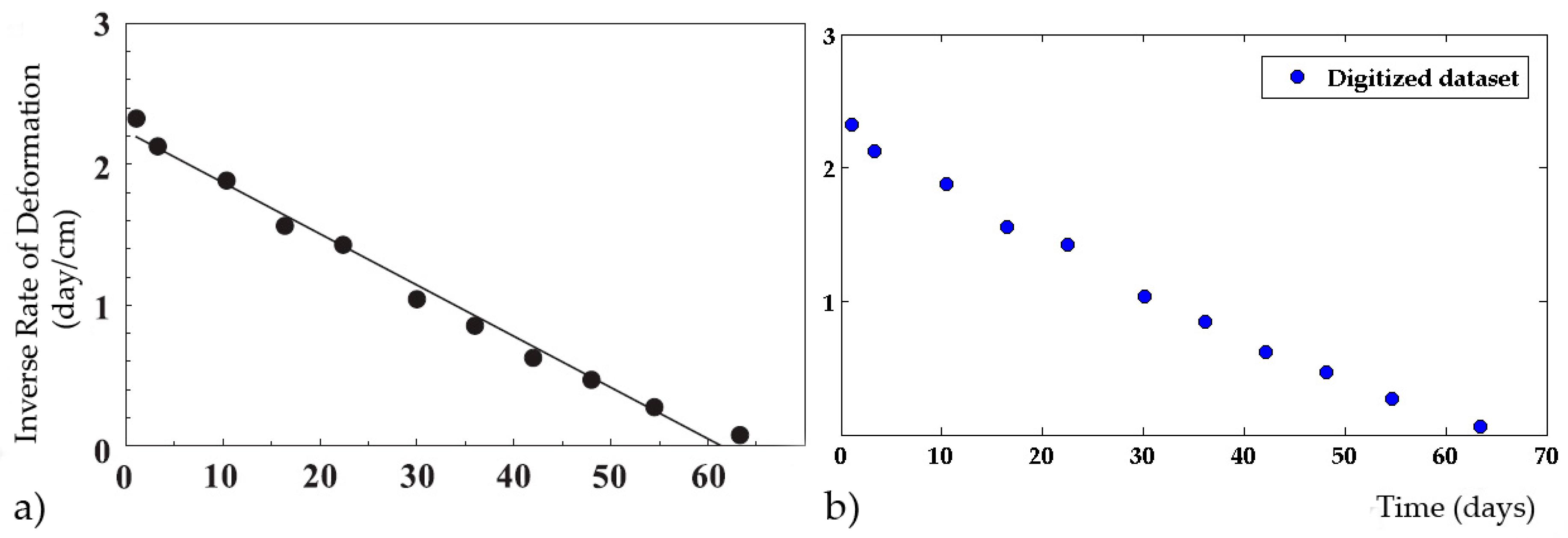
  • The digitization of the pre-failure datasets from graphs;
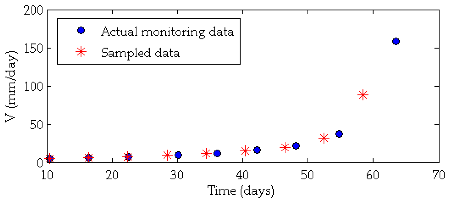
  • The sampling of 56 time series of displacements based on different satellites’ revisit time to reproduce the satellite data acquisition;
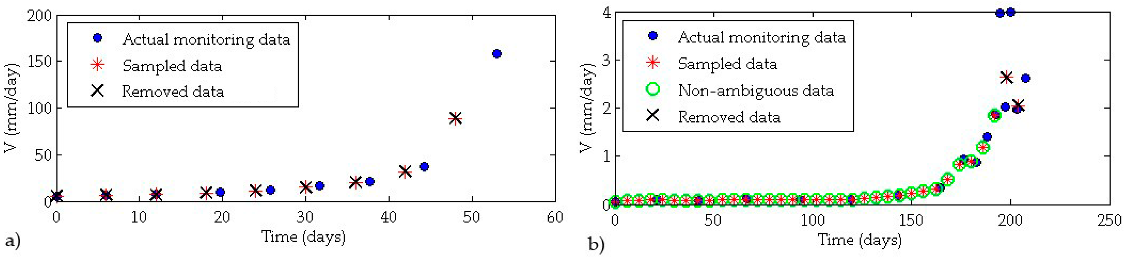
  • Simulation of the phase ambiguity constraint based on the different satellites’ features (wavelength and revisit time);
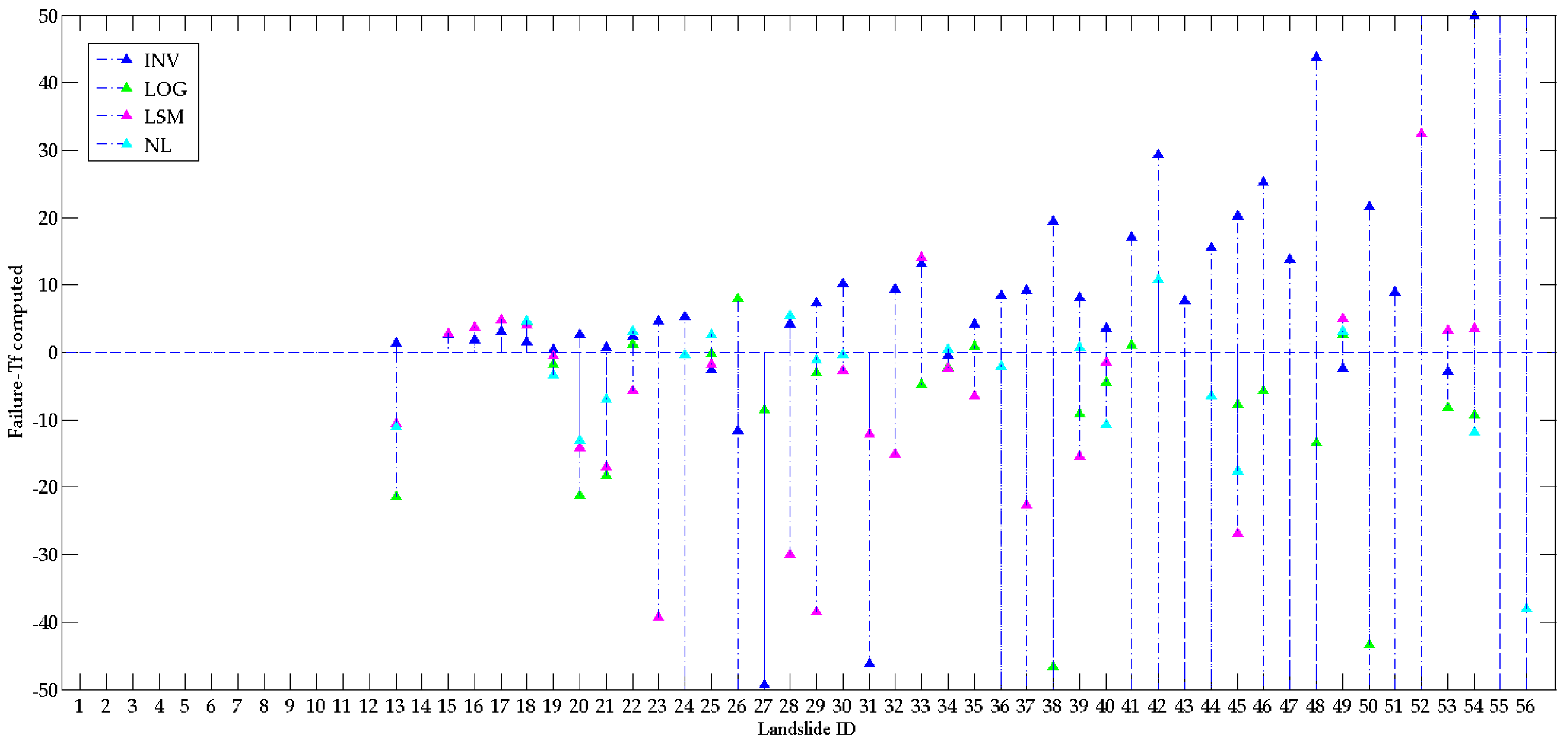
  • The application of four FFMs on three different datasets: (i) digitized datasets, which represent the actual monitoring datasets; (ii) sampled datasets (based on the revisit time constraint); and (iii) simulated datasets (considering the phase ambiguity limit);
  • A comparison between the forecast results obtained using actual monitoring data and simulated satellite data.
The pre-failure monitoring data of 56 past landslides have been explored by observing their evolution from the beginning of the acceleration phase to the occurrence of failure.
The collected monitoring data show different characteristics; they were acquired using different monitoring instruments (i.e., extensometers, inclinometers, distometers, GB-InSAR, and total station) and were displayed in the instruments using different formats, including displacement vs. time, velocity vs. time, and inverse velocity vs. time. Furthermore, the data was displayed in different units such as millimetres, centimetres, metres, mm/day, mm/hour, and cm/day. To homogenize the information and to compare the results, all the datasets are reported in mm/day.
The 56 landslide datasets collected (Table 1) show different features in terms of: triggering factor, mechanism, volume, material, and deformational behaviour.
For the objective of this work, the most important feature is the deformational behaviour of the slope before failure; specifically, the TC duration and the deformation rates occurring during the TC. The beginning of TC has been manually defined on the strain rate vs. time plot as the point at which the velocity begins to increase just before the final collapse. As shown in Table 1, the length of the TC period is extremely variable, ranging from several minutes to more than 1000 days. Additionally, the average velocity during the pre-failure phase varies substantially from 0.01 m/day to more than 4 m per day.
Monitoring data presented graphically in the scientific literature have been digitized using the MATLAB® code “grabit”. An example of the digitized data for the Vajont landslide is shown in Figure 1. To simulate the satellite data acquisition, the monitoring datasets of the 56 landslides have been sampled in the velocity time space based on different satellites’ RT values (Figure 2). The features of nine satellites in the past, present, and future have been considered (Table 2).
Furthermore, according to the satellites’ wavelengths and RT values, time series have been customized to consider the phase ambiguity limits. Because the phase is a periodic function and the wavelength number in the two travel paths is unknown, it follows that displacements greater than λ/2 between two consecutive acquisitions may remain unsolved or underestimated. Furthermore, for Advanced DInSAR (i.e., Persistent Scatterers Interferometry (PSI), Small Baseline Subset (SBAS), and similar techniques), the maximum amount of displacement that can be measured between two consecutive acquisitions is λ/4 [28]. To simulate this limit, we assumed that satellite InSAR is not able to monitor displacements greater than λ/4 between two consecutive acquisitions. For example, considering the Sentinel features, measurement points with displacements greater than 14 mm in 6 days have not been considered (Figure 3). Because the datasets are in the velocity–time space, the measurement points with a velocity greater than the velocity of ambiguity (Vambiguity) have been removed, where Vambiguity is defined as:
Vambiguity = (λ/4)/RT,
Four FFMs have been used to obtain the TF estimation [65]:
  • Inverse velocity method (INV, [6]);
  • Log rate vs. log acceleration technique (LOG, [11]);
  • Linearized least-square technique (LSM, [11]);
  • Non-linear least-square technique (NL, [11]).
The INV method is a graphical technique based on the linear approximation of the inverse velocity data, while the other methods are numerical techniques derived via the manipulation of Equation (1). The INV method is the most utilized due to its simple implementation in actual emergency situations. It works well for linearly distributed data (α = 2); however, the other methods allow data characterized by non-linear trends to be fit based on the estimation of the two constants A and α.
The four forecasting methods have been applied to all the landslide time series using the following datasets:
  • the actual monitoring data, i.e., the digitized datasets;
  • the sampled time series, i.e., the sampled time series based on the satellite’s revisit time;
  • the simulated time series, which considers the phase ambiguity constraint.
Using this approach, it was possible to assess the suitability of the satellite InSAR technique for monitoring the landslide process during the tertiary creep phase and for the application of FFMs based on the revisit time and phase ambiguity constraints of different satellite sensors.

3. Results

The FFM results are reported in the following subsections according to the datasets used: (i) the actual monitoring data (Section 3.1); (ii) the sampled data (Section 3.2) and (iii) the simulated time series (Section 3.3).

3.1. Actual Monitoring Data

The FFM results for the actual monitoring data are compared to the results obtained for the sampled and simulated time series. The forecasting methods have been applied to 56 past landslides considering all the tertiary creep phases from the beginning to the last available datum. For each landslide, the actual time of the slope failure (actual failure) is known, allowing us to estimate the prediction error. The prediction error obtained for each landslide according to each forecasting method is shown in Figure 4. The error (E) has been defined as the difference in days between the actual failure and the computed time of failure (Tf):
E = Actual Failure−Tf,
Based on this equation, positive error values would represent safe predictions in a priori analysis [29]; in contrast, negative error values are related to unsafe predictions (Tf is delayed with respect to the actual failure).
Landslide ID values are reported on the x-axis, while the prediction error is on the y-axis. ID values have been assigned according to an increasing TC length. Additionally, a decrease in data sampling frequency is contained in our database toward the higher ID values.
Figure 4 shows that the prediction error increases towards the higher ID values. Predictions close to the actual failure have been obtained for the low ID values (from ID 1 to ID 21), i.e., based on the datasets with higher sampling frequency and a short TC phase.
Overall, the semi-empirical methods returned predictions with an error less than 3 days for: 30 examples using the graphical technique, 28 using the NL technique, 24 using the LOG technique, and 15 using the LSM technique.

3.2. Sampled Datasets

For the application of forecasting methods, a minimum of three monitoring points within the accelerating phase is required. Under these conditions, we can build a function that can provide information on the increasing displacement velocity and, thus, we are able to apply semi-empirical models. Based on the TC duration and on the revisit time of the different satellites, the landslides with at least three data points within the TC phase have been defined as compatible for the application of the forecasting methods (Table 3).
Considering the past satellites (ALOS PALSAR, J-ERS, ERS, and Envisat) characterized by the longer revisit times ranging from 35 to 46 days, 14 compatible landslides (i.e., those that can be monitored using satellite InSAR) have been identified out of the 56 collected in the database. For the present and the future satellite generations, a maximum of 43 compatible landslides have been identified based on the revisit time of the Sentinel 1A-1B, Cosmo Sky-Med (theoretical RT of 4 days), and Radarsat Constellation.
Considering the present satellites’ features, the number of compatible landslides ranges from 26 to 43, i.e., from 25% to 86% of the landslides collected in the database. This means that, at present, considering only the revisit time constraint, we could observe a change in the displacement trend via satellite with at least three data points for more than 25% of the collected landslides, reaching 86% of the landslides considering the Sentinel-1 characteristics.
The four FFMs have been applied to every compatible landslide based on each satellite’s revisit time. Figure 5 shows the analysis performed considering the shorter revisit time (namely, 4 days), belonging to the future Radarsat Constellation and, theoretically, to the COSMO-SkyMed Constellation. For the forecasting analysis applied to the actual monitoring data, the prediction error increases toward the higher ID values. Specifically, the errors derived from the INV application are small (<±5 days) up to ID 25 and start to increase after ID 25.
Table 3 and Figure 6 show that the number of satisfactory predictions increases toward the shorter revisit times. A prediction is considered satisfactory if the prediction error is within ±5 days. The INV method shows the strongest relationship between the number of successful forecasts and the RT (Figure 6b), because a shorter RT results in a higher number of accurate predictions.
The analysis shows that the INV method results in a better accuracy for the TF estimation. The INV technique has a prediction error of less than 5 days for 17 landslides based on an RT of 4 days, and for 13 landslides based on the RT of the Sentinel-1 satellite.

3.3. Simulated Time Series

Considering the phase ambiguity constraints, a maximum of 24 compatible landslides out of the 56 have been identified based on the Radarsat Constellation features and characterized by the best association between the revisit time and the sensor’s wavelength. Currently, the Sentinel-1 constellation would have observed 17 landslides with at least three measurement points inside the acceleration phase preceding the slope collapse. By introducing the phase ambiguity, the suitability of the failure forecasting methods decrease. For the simulated satellite datasets, only a maximum of four satisfactory predictions have been obtained using the inverse velocity method (Table 4).

4. Discussion

The forecasting methods have great potential for landslide hazard management [16,18,19,20]. By applying FFMs to actual monitoring data, we have obtained a prediction error lower than 3 days in 53.7% of the examples using the INV method, 51.7% using the LOG technique, 48.2% using the NL technique, and 27.8% using the LSM technique. The percentage of successful predictions increases when considering landslides with shorter TC phases and datasets characterized by a higher sampling frequency, namely, the landslide database presented here with lower ID values. When considering only the first 21 landslides (TC < 15 days), an error lower than 3 days has been obtained in 100% of the examples using the INV method, 85.7% using the LOG technique, 76.2% using the NL technique, and 57.1% using the LSM method.
For the sampled and simulated datasets, the number of successful predictions decreases (Table 3 and Table 4). Only a maximum of four satisfactory predictions have been obtained with the inverse velocity method including the ambiguity phase constraints. The principal reason is because the FFMs have been applied to only the landslides with a TC phase long enough to be observed with the satellite’s RT (high ID values). The predictions obtained using the actual and simulated datasets are similar (Figure 7) when the FFMs are accurate using the actual monitoring data (ID 23, 27, 35, 49, 53). A reliable prediction can also be obtained using the simulated datasets; however, if the prediction error is high using the actual time series, the FFMs fail using the simulated satellite data as well.
The error growth towards higher ID values could be related to both the decrease of the data sampling frequency and to the increase of the TC phase duration. Because of the inverse relationship between the TC length and data sampling frequency (Figure 8), we are not able to clearly determine which parameter primarily affects the success or the failure of the forecasting analyses. A higher sampling frequency produces more robust datasets for the application of forecasting methods, especially near the time of slope collapse; however, a very long TC phase can lead to complex deformational behaviours due to the variation of the stress conditions, which has a negative impact on the FFM stability. The difference in the prediction errors obtained with the actual and simulated time series data is related to the loss of the last monitoring data caused by the sampling and ambiguity phase reproduction. It is assumed that the last monitoring data before the collapse significantly affects the forecasting analyses results because they include the highest velocity of the phenomenon. Under equal conditions, the closer the monitoring data are to the actual slope failure time, the more accurate the forecast. This can be proven by comparing the predictions obtained using the entire time series (datasets from the beginning of TC until the last monitoring datum) and only a part of the time series (i.e., removing the last measurement points) (Figure 9). Based on our results, there is a connection between the time intervals from the last available measurement point to the actual failure (GAP) and the accuracy of the forecasting methods. The relationship between the GAP and the prediction accuracy can be observed for the majority of the landslides collected (Figure 9a,b). In Figure 9c, an example is shown where the prediction accuracy increases when approaching the actual failure based on the Preonzo landslide monitoring data.
The GAP reduction capability is related to the sampling frequency; the higher the sampling frequency, the greater the ability to obtain measurements closer to the actual failure. Figure 10 shows the relationship between the GAP and the sampling frequency for the time series of our database.

5. Conclusions

From our analyses, the following conclusions can be drawn:
  • Monitoring sampling frequency is important for the application of forecasting methods. For some events, an accurate prediction using FFMs on simulated satellite data has been obtained. However, satellite interferometry cannot provide, at present, the sampling frequency required for a reliable FFM for early warning purposes.
  • Satellite interferometry has potential for monitoring landslide precursors and for detecting the slopes affected by a change in their deformational behaviour. According to the deformational behaviours of our landslide database, at present, 30% of the events could have been monitored during the acceleration phase with at least three data points, even considering the phase ambiguity constraints. Thus, based on the Sentinel 1A + 1B features, it is possible to monitor 17/56 landslides using satellite SAR interferometry.
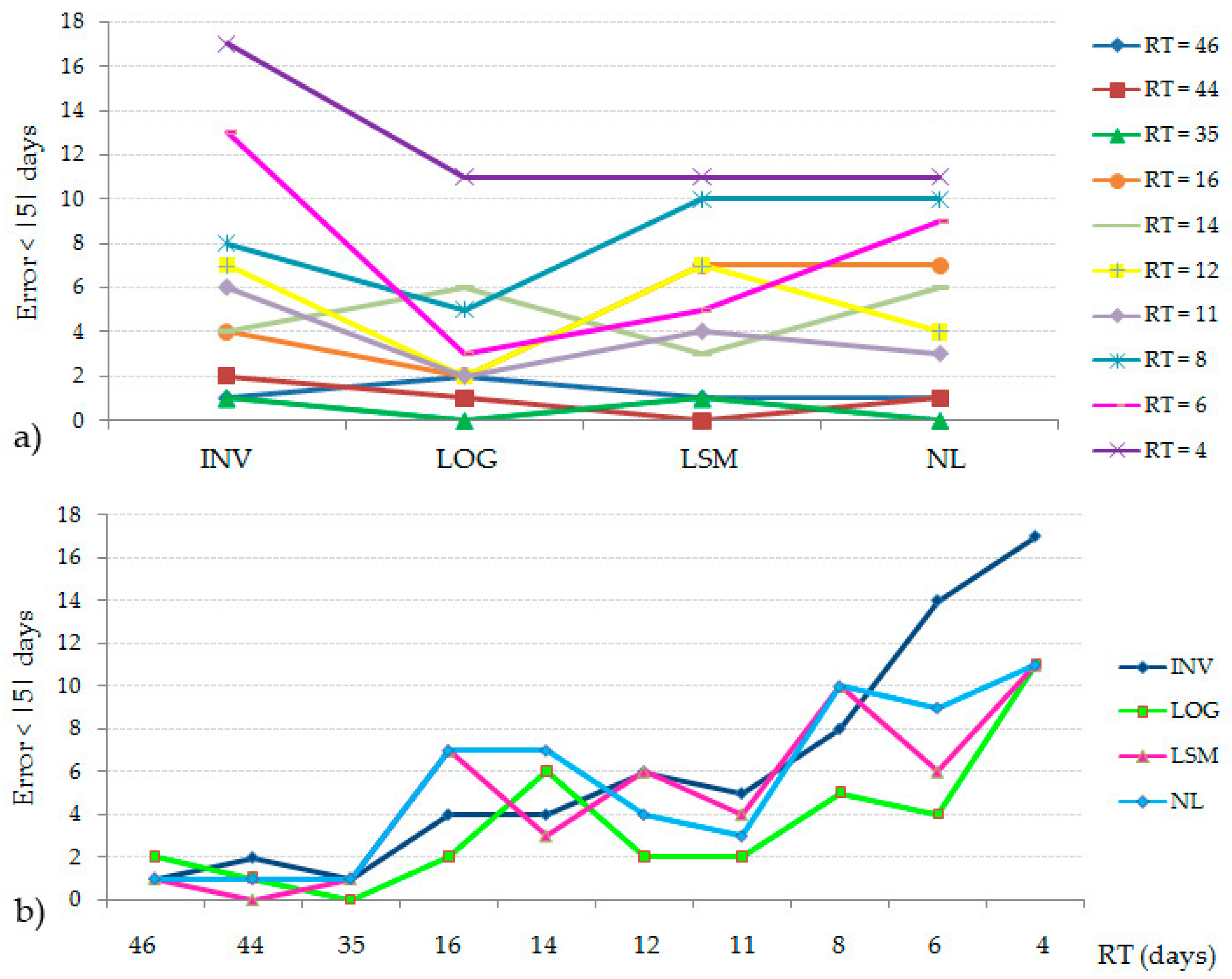
  • Considering both the RT and ambiguity phase limits, it would have been possible to forecast a maximum of 4 landslides with an error smaller than 5 days, based on the Sentinel-1 features. This is due to the strong constraints related to the phase ambiguity, which does not allow the monitoring of the high displacement rate occurring during the tertiary creep phase. Notably, it is sometimes possible to monitor consecutive displacements greater than λ/4. If one direction of motion can be assumed (‘upward’ or ‘downward’, as for the majority of landslides), the maximum measurable displacement between a pair of scenarios becomes one-half of the wavelength [28,29]. However, considering λ/2 as the maximum detectable displacement between two consecutive acquisitions, we achieved a similar result: six successful forecasts were obtained based on the Sentinel-1 features.
  • If a landslide process is monitored using a suitable technique (high spatial and temporal resolution), forecasting methods can be a powerful tool for risk management and for early-warning systems.

Acknowledgments

The present work has been carried out in the framework of the project “Grandi Frane in roccia e Frane Superficiali a Cinematica Rapida in Aree Montane: Metodi Per La Previsione Temporale e Spaziale (Prediction and Susceptibility)”, supported by the Dipartimento per gli Affari Regionali e le Autonomie della Presidenza del Consiglio dei Ministri and the Università di Roma «La Sapienza». We would like to thank the two anonymous reviewers and the Editor for their helpful and constructive comments.

Author Contributions

Francesca Bozzano and Paolo Mazzanti conceived the study. Francesca Bozzano, Carlo Esposito and Paolo Mazzanti coordinated the research and contributed to the article organization. Serena Moretto and Alfredo Rocca built the landslides database. Serena Moretto designed and performed the forecasting analyses. Serena Moretto and Francesca Bozzano drafted the manuscript which was revised by all Authors.

Conflicts of Interest

The authors declare no conflict of interest.

References

  1. Heim, A. Bergsturz und Menschenleben; Fretz. & Wasmuth: Zürich, Switzerland, 1932. (In Germany) [Google Scholar]
  2. Terzaghi, K. Mechanism of landslides. In Application of Geology to Engineering Practice (Berkeley Volume); Geological Society of America: Washington, DC, USA, 1950; pp. 83–123. [Google Scholar]
  3. Saito, M.; Uezawa, H. Failure of Soil due to Creep. In Proceedings of the 5th International Conference on Soil Mechanics and Foundation Engineering (ICSMFE), Paris, France, 17–22 July 1961; Volume 1, pp. 315–318. [Google Scholar]
  4. Saito, M. Forecasting the Time of Occurrence of a Slope Failure. In Proceedings of the 6th International Conference on Soil Mechanics and Foundatin Engineering, Montreal, QC, Canada, 8–15 September 1965; pp. 537–541. [Google Scholar]
  5. Voight, B.; Kennedy, B.A. Slope Failure of 1967–1969, Chuquicamata Mine, Chile. Dev. Geotech. Eng. 1979, 4, 595–632. [Google Scholar]
  6. Fukuzono, T. A new method for predicting the failure time of a slope. In Proceedings of the 4th International Conference and Field Workshop on Landslides, Tokyo, Japan, 23–31 August 1985; pp. 145–150. [Google Scholar]
  7. Azimi, C.; Biarez, J.; Desvarreux, P.; Keime, F. Forecasting time of failure for a rockslide in gypsum. In Proceedings of the 5th international symposium on landslides, Lausanne, Switherland, 10–15 July 1988; pp. 531–536. [Google Scholar]
  8. Voight, B. A relation to describe rate-dependent material failure. Science 1989, 243, 200–203. [Google Scholar] [CrossRef] [PubMed]
  9. Voight, B. A method for prediction of volcanic eruptions. Nature 1988, 332, 125–130. [Google Scholar] [CrossRef]
  10. Fukuzono, T. A simple method for predicting the failure time of slope using reciprocal of velocity. Technol. Disaster Prev. Sci. Technol. Agency Jpn. Int. Coop. Agency 1989, 13, 111–128. [Google Scholar]
  11. Cornelius, R.R.; Voight, B. Graphical and PC-software analysis of volcano eruption precursors according to the materials failure forecast method (FFMS). J. Volcanol. Geotherm. Res. 1995, 64, 295–320. [Google Scholar] [CrossRef]
  12. Kilburn, C.R.; Petley, D.N. Forecasting giant, catastrophic slope collapse: Lessons from Vajont, Northern Italy. Geomorphology 2003, 54, 21–32. [Google Scholar] [CrossRef]
  13. Petley, D.N.; Higuchi, T.; Petley, D.J.; Bulmer, M.H.; Carey, J. Development of progressive landslide failure in cohesive materials. Geology 2005, 33, 201–204. [Google Scholar] [CrossRef]
  14. Petley, D.N.; Petley, D.J.; Allison, R.J. Temporal prediction in landslides. Understanding the Saito effect. In Landslides and Engineered Slopes: From the Past to the Future; Taylor & Francis: Xi’an, China, 2008; pp. 794–800. [Google Scholar]
  15. Rose, N.D.; Hungr, O. Forecasting potential rock slope failure in open pit mines using the inversevelocity method. Int. J. Rock Mech. Min. Sci. 2007, 44, 308–320. [Google Scholar] [CrossRef]
  16. Gigli, G.; Fanti, R.; Canuti, P.; Casagli, N. Integration of advanced monitoring and numerical modeling techniques for the complete risk scenario analysis of rockslides: The case of Mt. Beni (Florence, Italy). Eng. Geol. 2011, 120, 48–59. [Google Scholar] [CrossRef]
  17. Bozzano, F.; Cipriani, I.; Mazzanti, P.; Prestininzi, A. A field experiment for calibrating landslide time-of-failure prediction functions. Int. J. Rock Mech. Min. Sci. 2014, 67, 69–77. [Google Scholar] [CrossRef]
  18. Mazzanti, P.; Bozzano, F.; Cipriani, I.; Prestininzi, A. New insights into the temporal prediction of landslides by a terrestrial SAR interferometry monitoring case study. Landslides 2015, 12, 55. [Google Scholar] [CrossRef]
  19. Manconi, A.; Giordan, D. Landslide early warning based on failure forecast models: The example of the Mt. de La Saxe rockslide, northern Italy. Nat. Hazards Earth Syst. Sci. 2015, 15, 1639–1644. [Google Scholar] [CrossRef]
  20. Sättele, M.; Krautblatter, M.; Bründl, M.; Straub, D. Forecasting rock slope failure: How reliable and effective are warning systems? Landslide 2016, 13, 737. [Google Scholar] [CrossRef]
  21. Loew, S.; Gschwind, S.; Keller-Signer, A.; Valenti, G. Monitoring and Early Warning of the 2012 Preonzo Catastrophic Rockslope Failure. Landslides 2017, 14, 141. [Google Scholar] [CrossRef]
  22. Ferretti, A.; Prati, C.; Rocca, F. Nonlinear subsidence rate estimation using permanent scatterers in differential SAR interferometry. IEEE Trans. Geosci. Remote Sens. 2000, 38, 2202–2212. [Google Scholar] [CrossRef]
  23. Ferretti, A.; Prati, C.; Rocca, F. Permanent scatterers in SAR interferometry. IEEE Trans. Geosc. Remote Sens. 2001, 39, 8–20. [Google Scholar] [CrossRef]
  24. Berardino, P.; Fornaro, G.; Lanari, R.; Sansosti, E. A new algorithm for surface deformation monitoring based on small baseline differeential SAR interferograms. IEEE Trans. Geosc. Remote Sens. 2002, 40, 2375–2383. [Google Scholar] [CrossRef]
  25. Perissin, D.; Wang, T. Repeat-Pass SAR Interferometry with Partially Coherent Targets. IEEE Trans. Geosci. Remote Sens. 2012, 50, 271–280. [Google Scholar] [CrossRef]
  26. Early Warning from Space of Homes on the Slide. Available online: http://www.esa.int/Our_Activities/Observing_the_Earth/Early_warning_from_space_of_homes_on_the_slide (accessed on 9 May 2017).
  27. Mazzanti, P.; Rocca, A.; Bozzano, F.; Cossu, R.; Floris, M. Landslides Forecasting Analysis by Time Series Displacement Derived from Satellite InSAR Data: Preliminary Results. In Proceedings of the Fringe 2011, Frascati, Italy, 19–23 September 2011. [Google Scholar]
  28. Ferretti, A.; Prati, C.; Rocca, F.; Nicola, C.; Farina, P.; Young, B. Permanent scatterers technology: A powerful state of the art tool for historic and future monitoring of landslides and other terrain instability phenomena. In International Conference on Landslide Risk Management; Balkema: Vancouver, BC, Canada, 2005. [Google Scholar]
  29. Crosetto, M.; Monserrat, O.; Iglesias, R.; Crippa, B. Persistent scatterer interferometry: Potential, limits and initial cand X-band comparison. Photogramm. Eng. Remote Sens. 2010, 76, 1061–1069. [Google Scholar] [CrossRef]
  30. Fukuzono, T. Experimental Study of Slope Failure Caused by Heavy Rainfall. IAHS-AISH Publ. 1987, 165, 133–134. [Google Scholar]
  31. Moriwaki, H.; Inokuchi, T.; Hattanji, T.; Sassa, K.; Ochiai, H.; Wang, G. Failure processes in a full-scale landslide experiment using a rainfall simulator. Landslides 2012, 1, 277–288. [Google Scholar] [CrossRef]
  32. Mufundirwa, A.; Fujii, Y.; Kodama, J. A new practical method for prediction of geomechanical failure-time. Int. J. Rock Mech. Min. Sci. 2010, 47, 1079–1090. [Google Scholar] [CrossRef]
  33. Kayesa, G. Prediction of slope failure at Letlhakane mine with the geomos slope monitoring system. In International Symposium on Stability of Rock Slopes in Open Pit Mining and Civil Engineering; The South African Institute of Mining and Metallurgy: Johannesburg, South Africa, 2006; pp. 606–622. [Google Scholar]
  34. Saito, M. Forecasting Time of Slope Failure by Tertiary Creep. In Proceedings of the 7th International Conference on Soil Mechanics and Foundation Engineering; Sociedad Mexicana de Mecanica: Mexico City, Mexico, 1969; pp. 677–683. [Google Scholar]
  35. Manconi, A.; Giordan, D. Landslide failure forecast in near-real-time. Geomat. Nat. Hazard. Risk 2014, 7, 639–648. [Google Scholar] [CrossRef]
  36. Kent, A. Coal mine waste dumps in British Columbia stability issues and recent developments. Int. Mine Waste Manag. 1992, 10–18. [Google Scholar]
  37. Iovine, G.; Petrucci, O.; Rizzo, V.; Tansi, C. The march 7th 2005 Cavallerizzo (Cerzeto) Landslide in Calabria—Southern Italy. In Proceedings of the 10th IAEG Congress, Nottingham, UK, 6–10 September 2006; pp. 1–12. [Google Scholar]
  38. Okamoto, T.; Larsen, J.O.; Matsuura, S.; Asano, S.; Takeuchi, Y.; Grande, L. Displacement properties of landslide masses at the initiation of failure in quick clay deposits and the effects of meteorological and hydrological factors. Eng. Geol. 2004, 72, 233–251. [Google Scholar] [CrossRef]
  39. Thompson, P.W. Confirmation of a Failure Mechanism Using Open Pit Monitoring Methods. In Proceedings of the Australian Conference on Geotechnical Instrumentation and Monitoring in Open Pit and Underground Mining, Kalgoorlie, Australia, 21–23 June 1993; pp. 483–489. [Google Scholar]
  40. Glastonbury, B.; Fell, R. Report on the Analysis of the Deformation Behaviour of Excavated Rock Slopes; School of Civil & Environmental Engineering, University of New South Wales: Sydney, Australia, 2002. [Google Scholar]
  41. GEOPRAEVENT. Available online: www.geopraevent.ch (accessed on10 May 2017).
  42. Metodi Innovativi per il Controllo e la Gestione dei Fenomeni Franosi. Available online: http://www.eventi.saie.bolognafiere.it/media/saie/presentazioni%20sba/sala%20A/Matteo_Berti.pdf (accessed on 10 May 2017). (In Italian).
  43. Ulusay, R.; Aksoy, H. Assessment of the failure mechanism of a highwall slope under spoil pile loadings at a coal mine. Eng. Geol. 1994, 38, 117–134. [Google Scholar] [CrossRef]
  44. Ryan, T.M.; Call, R.D. Applications of Rock Mass Monitoring for Stability Assessment of Pit Slope Failure. In Proceedings of the 33th U.S. Symposium on Rock Mechanics (USRMS), Santa Fe, NM, USA, 3–5 June 1992; Balkema: Rotterdam, The Netherlands, 1992. [Google Scholar]
  45. Cahill, J.; Lee, M. Ground control at Leinster nickel operations. In International Symposium on Stability of Rock Slopes in Open Pit Mining and Civil. Engineering; The South African Institute of Mining and Metallurgy: Johannesburg, South Africa, 2006; pp. 321–334. [Google Scholar]
  46. Salt, G. Landslide Mobility and Remedial Measures. In Proceedings of the 5 International Symposium on Landslides, Rotterdam, The Netherlands, 1988; pp. 757–762. [Google Scholar]
  47. Carey, J.M.; Moore, R.; Petley, D.N.; Siddle, H.J. Pre-failure behaviour of slope materials and their significance in the progressive failure of landslides. In Landslides and Climate Change: Challenges and Solutions; Taylor & Francis Group: London, UK, 2007; pp. 207–215. [Google Scholar]
  48. Urcioli, G.; Picarelli, L. Interaction between landslides and man-made works. In Landslides and Engineered Slopes; Taylor & Francis Group: London, UK, 2008. [Google Scholar]
  49. Borsetto, M.; Frassoni, A.; La Barbera, G.; Fanelli, M.; Giuseppetti, G.; Mazzà, G. An application of Voight empirical model for the prediction of soil and rock instabilities. In Proceedings of the 7th International Symposium on Landslides; Bell, D.H., Ed.; Balkema: Rotterdam, The Netherlands; Christchurch, New Zealand, 1991; pp. 335–341. [Google Scholar]
  50. Petley, D.N. The evolution of slope failures: Mechanisms of rupture propagation. Nat. Hazard. Earth Sys. Sci. 2004, 4, 147–152. [Google Scholar] [CrossRef]
  51. Bai, J.G.; Lu, S.D.; Han, J.S. Importance of study of creep sliding mechanism to prevention and treatment of reservoir landslide. In Landslides and Engineered Slopes: From the Past to the Future; Taylor & Francis Group: Xi’an, China, 2008; pp. 1071–1076. [Google Scholar]
  52. Bhandari, R.K. Special lecture—Some practical lessons in the investigation and field monitoring of landslides. Landslides 1988, 1–3, 1435–1457. [Google Scholar]
  53. Zavodni, Z.M.; Broadbent, C.D. Slope failure kinematics. CIM Bull. 1980, 69–74. [Google Scholar]
  54. Brawner, C.O.; Stacey, P.F. Hogarth pit slope failure, Ontario, Canada. In Rockslides and Avalanches, B; Elsevier: Amsterdam, The Netherlands, 1979; pp. 691–707. [Google Scholar]
  55. Glastonbury, B.; Fell, R. Report On the Analysis of Rapid Natural Rock Slope. R-390; School of Civil & Environmental, University of New South Wales (UNSW): Sydney, Australia, 2001. [Google Scholar]
  56. Brown, I.; Hittinger, M.; Goodman, R. Finite element study of the Nevis Bluff (New Zealand) rock slope failure. Rock Mech. 1980, 12, 231–245. [Google Scholar] [CrossRef]
  57. Keqiang, H.; Sijing, W. Double-parameter threshold and its formation mechanism of the colluvial landslide: Xintan landslide, China. Environ. Geol. 2006, 49, 696–707. [Google Scholar] [CrossRef]
  58. Schumm, S.A.; Chorley, R.J. The fall of Threatening Rock. Am. J. Sci. 1964, 262, 1041–1054. [Google Scholar] [CrossRef]
  59. D’Elia, B.; Picarelli, L.; Leroueil, S.; Vaunat, J. Geotechnical characterisation of slope movements in structurally complex clay soils and stiff jointed clays. Riv. Ital. Geotec. 1998, 3, 5–47. [Google Scholar]
  60. Zabusky, L.; Swidzinski, W.; Kulczykowski, M.; Mrozek, T.; Laskowicz, I. Monitoring of landslides in the Brada river valley in Koronowo (Polish Lowlands). Environ. Earth Sci. 2015, 73, 8609–8619. [Google Scholar] [CrossRef]
  61. Boyd, J.M.; Hinds, D.V.; Moy, D.; Rogers, C. Two simple devices for monitoring movements in rock slopes. Quart. J. Eng. Geol. Hydrogeol. 1973, 6, 295–302. [Google Scholar] [CrossRef]
  62. Siqing, Q.; Sijing, W. A homomorphic model for identifying abrupt abnormalities of landslide forerunners. Eng. Geol. 2000, 57, 163–168. [Google Scholar] [CrossRef]
  63. Royán, M.J.; Abellán, A.; Vilaplana, J.M. Progressive failure leading to the 3 December 2013 rockfall at Puigcercós scarp (Catalonia, Spain). Landslides 2015, 12, 585–595. [Google Scholar] [CrossRef]
  64. Muller, L. The rock slide in the Vaiont valley. Felsmech. Ing. 1964, 42, 148–212. [Google Scholar]
  65. Bozzano, F.; Mazzanti, P.; Esposito, C.; Moretto, S.; Rocca, A. Potential of satellite InSAR monitoring for landslide Failure Forecasting. In Landslides and Engineered Slopes. Experience, Theory and Practice; CRC Press: Boca Raton, FL, USA, 2016; Volume 2, pp. 523–530. [Google Scholar]
  66. Moretto, S.; Bozzano, F.; Esposito, C.; Mazzanti, P. Lesson learned from the pre-collapse time series of displacement of the Preonzo landslide (Switzerland). Rend. Online Soc. Geol. Ital. 2016, 41, 247–250. [Google Scholar] [CrossRef]
Figure 1. An example of the digitized monitoring data for the Vajont landslide (9 October 1963). (a) Monitoring data available in the literature ([12] after Muller [64] and Voight [8]) referencing the inverse rates (days/cm) of horizontal slope movement registered before the Mt. Toc catastrophic collapse. Velocity measurements were obtained from stations near the toe of the moving mass [12]; (b) Digitized data.
Geosciences 07 00036 g001
Figure 2. Example of sampled datasets (red stars) based on the Sentinel 1A + 1B revisit time of 6 days. Blue circles represent the pre-failure monitoring data of the Vajont landslide.
Geosciences 07 00036 g002
Figure 3. An example of the ambiguity phase simulation based on the Sentinel 1A+1B features (RT = 6 days and Vambiguity = 2.33 mm/day). Removed data (black X) represent the measurements with a velocity greater than the velocity of ambiguity, while the green circles represent data with V < Vambiguity. (a) Vajont’s datasets; in this case, the deformations occurring during the pre-failure stage were too fast to be monitored with satellite interferometry; (b) Excavation C datasets. The raw data consist of surface displacement data acquired using a prism monitoring system.
Geosciences 07 00036 g003
Figure 4. Error diagram obtained for the actual monitoring datasets. The colours identify the different failure forecasting methods (FFMs).
Geosciences 07 00036 g004
Figure 5. Diagram of the prediction error for the compatible landslides based on a RT of 4 days.
Geosciences 07 00036 g005
Figure 6. (a) Relationship between the number of successful forecasts and the forecasting method considering the different revisit times; (b) Relationship between the revisit time and the number of satisfactory predictions based on each FFM.
Geosciences 07 00036 g006
Figure 7. Comparison between the INV method applied to the actual monitoring data and to the simulated datasets. The results of the simulated datasets are referenced to the Sentinel 1A + 1B features.
Geosciences 07 00036 g007
Figure 8. Inverse correlation between the TC’s length and data sampling frequency.
Geosciences 07 00036 g008
Figure 9. Prediction errors. (a) Errors using the INV method to: (i) the entire available time series (green predictions) and (ii) removing the last three measurement points (blue predictions); (b) Prediction error vs. GAP (time interval between the last datum and the actual failure); (c) INV iterative forecasting analysis for the Preonzo Landslide (ID 12) (modified after [66]). The predictions have been updated by simulating the data acquisition over time. The time of the actual failure (15 May) is displayed as a red dashed line. The critical line (red line) corresponds to the day the forecast was made. Consequently, it represents the lower boundary of a reasonable prediction. The analysis shows that the closer the last available datum is to the actual failure, the more accurate the prediction. When approaching the actual failure, the prediction error decreases, in this case, following a linear trend for the INV methods.
Geosciences 07 00036 g009
Figure 10. Relationship between the data sampling frequency and the GAP for the collected landslide database.
Geosciences 07 00036 g010
Table 1. Landslide database collected from the scientific literature.
LandslideReferenceIDTertiary Creep (TC) Length (days)Average Velocity (mm/day)
Jitsukiyama[30]10.010.04 (mm/s)
Moriwaki Experiment[31]20.020.04 (mm/min)
Unnamed Mufundirawa[32]30.10.87 (mm/s)
Letlhakane Mine[33]40.268.60 (mm/h)
Dosan Line[34]51.2664.79
La Saxe[35]61.64541.68
Betz Post 2 mc[15]73.263.42
Asamushi[34]83.4163.76
Rock Dump[36]94.11011.21
Cavallerizzo[37]104.326.32
Roesgrenda B[38]116171.93
Tuckabianna West[39]126.139.55
Afton[40]139.4591.07
Excavation A[40]149.714.22
Preonzo[41]1510.691.30
Silla Montecchi[42]1610.880.31
Eskihisar Coal Mine[43]1711.56.72
Ryan Call Slide1[44]1812.81564.10
Crack Gauge[45]191311.98
Ruahihi[46]2014.154.58
Es.2 Rose & Hungr2007[15]211552.16
Roesgrenda A[38]2220.12.00
Abbotsford[46]2320.4106.26
New Tredegar[47]2422.536.22
Victorious East Pit[40]2522.74.56
Haveluck[40]2625.81.94
Bohemia[48]2730.30.51
Val Pola[49]2830.551.33
Luscar_51B2[40]2931.676.73
Ooigawa Railroad[34]3038.912.76
Telfer[40]3139.42.73
Liberty Pit Mine[15]3240.24.73
Selbourn[50]3341.5100.54
Betz Post 18mc[15]34446.58
Lijiaxia[51]3544.74.47
Takabayama[52]3644.9145.78
Kennekott#1[53]3746.957.19
Chuquicamata Mine2[52]3847.6224.24
Ryan Call Slide2[44]3953.721.35
Vajont[13]4054.630.41
Luscar 50A2[40]4160.91272.11
Hogart[54]4277.863.85
Roberts[55]4310557.46
Nevis Bluff[56]44110.42.98
Monte Beni[16]45132.219.67
Xintan[57]46138.9459.60
Azimi 1988[7]47143.83.39
Threatening Rock[58]48153.82.49
Bomba[59]49167.910.86
Smoky River[40]50174.21.59
Scalate[55]51183.70.76
Brada River[60]52187.80.10
Excavation C[40]53211.31.22
Delabole Quarry[61]54380.72.89
Saleshan[62]55631.31.88
Puigcercos Scarp[63]5610130.39
Table 2. Satellites considered in this study and their principal features (Revisit Time (RT) and wavelength (λ)).
PeriodSatelliteRevisit Time (days)Bandλ (mm)
PastALOS PALSAR 146L236
J-ERS44L235
ERS 1/2-Envisat35C56
PresentCOSMO-SkyMed4X31
8X31
16X31
Sentinel-1A12C56
Sentinel 1A + 1B6C56
ALOS PALSAR 214L236
TerraSAR-X11X31
FutureRadarsat Constellation4C56
Table 3. Analysis results for the sampled datasets related to different RTs. The number of compatible landslides and the number of satisfactory predictions (error lower than ±5 days) for each satellite are reported. The compatible landslides include at least three data samples in the TC phase. For each forecasting method (inverse velocity method—INV, log rate vs. log acceleration technique—LOG, linearized least-square technique—LSM, and non-linear least-square technique—NL), the number of landslides with a prediction error lower than ±5 days is reported. The best performances obtained in terms of prediction accuracy are underlined.
PeriodSatelliteRT (Days)Bandλ (mm)Compatible Landslides
(Revisit Time)
E < |5| Days INVE < |5| Days LOGE < |5| Days LSME < |5| Days NL
Number of Landslides
PastALOS PALSAR 146L236141211
J-ERS44L235142101
ERS 1/2-Envisat35C56141010
PresentCOSMO-SkyMed4X314317111111
8X3135851010
16X31264277
Sentinel-1A12C56307274
Sentinel 1A + 1B6C563813359
ALOS PALSAR 214L236294636
TerraSAR-X11X31306243
FutureRadarsat Constellation4C564317111111
Table 4. Analysis results introducing the phase ambiguity constraint based on the different satellite’s features. “Compatible Landslides (Phase ambiguity)” represents the number of landslides with at least three data points in the TC phase accounting for the phase ambiguity limit. For each forecasting method, the number of landslides with a prediction error lower than 5 days is reported.
PeriodSatelliteRT (days)Bandλ (mm)Compatible Landslides (RT)Compatible Landslides (Phase Ambiguity)E < |5| days INVE < |5| days LOGE < |5| days LSME < |5| days NL
Number of Landslides
PastALOS PALSAR 146L2361470100
J-ERS44L2351480000
ERS ½-Envisat35C561441010
PresentCOSMO-SkyMed4X3143193031
8X3135110020
16X312690000
Sentinel-1A12C5630111000
Sentinel 1A + 1B6C5638174321
ALOS PALSAR 214L23629141211
TerraSAR-X11X313090000
FutureRadarsat Constellation4C5643244142

