Evolution of Neural Dynamics in an Ecological Model


School of Informatics and Computing, Indiana University, 919 E. 10th St., Bloomington, IN 47408, USA
*
Author to whom correspondence should be addressed.
Geosciences 2017, 7(3), 49; https://doi.org/10.3390/geosciences7030049
Submission received: 14 March 2017
/
Revised: 20 June 2017
/
Accepted: 27 June 2017
/
Published: 4 July 2017
(This article belongs to the Special Issue Individual-Based Ecological Modeling)
Abstract
:What is the optimal level of chaos in a computational system? If a system is too chaotic, it cannot reliably store information. If it is too ordered, it cannot transmit information. A variety of computational systems exhibit dynamics at the “edge of chaos”, the transition between the ordered and chaotic regimes. In this work, we examine the evolved neural networks of Polyworld, an artificial life model consisting of a simulated ecology populated with biologically inspired agents. As these agents adapt to their environment, their initially simple neural networks become increasingly capable of exhibiting rich dynamics. Dynamical systems analysis reveals that natural selection drives these networks toward the edge of chaos until the agent population is able to sustain itself. After this point, the evolutionary trend stabilizes, with neural dynamics remaining on average significantly far from the transition to chaos.
1. Introduction
1.1. Chaos and Its Edge
Two hallmarks of chaos are aperiodicity and sensitive dependence on initial conditions [1]. The former indicates that chaotic systems appear disordered; it is difficult to find patterns in their behavior even if they are completely deterministic. The latter indicates that arbitrarily similar initial states eventually yield wildly different outcomes; long-term prediction of a chaotic system’s behavior is thus impossible.
Many systems are capable of exhibiting both ordered and chaotic activity. The behavior of such a system is often governed by control parameters—variables that, when manipulated, can cause chaos to appear or disappear [1]. The “edge of chaos” refers to the transition between the ordered and chaotic regimes.
Edge-of-chaos dynamics are found in many computational systems, both artificial [2,3,4] and biological [5,6,7]. For example, in his analysis of one-dimensional cellular automata, Langton [2] suggested that information storage, modification, and transmission are most effective in systems approaching—but not fully reaching—chaos. Of particular relevance to the present study is the work of Bertschinger and Natschläger [4], who showed that recurrent neural networks capable of performing complex computations exhibit dynamics at the edge of chaos. In an example from biology, Skarda and Freeman [5] proposed that chaotic activity in the neural dynamics of rabbits serves as a ground state for olfactory perception, but only when this activity is constrained to low magnitudes.
These findings suggest that systems at the edge of chaos are better suited for information processing, and that, if computational systems are permitted to self-organize, they may do so near this transition [8,9]. Systems in this state are ordered enough to reliably store information, yet not so rigid that they cannot transmit it [10]. However, it is important to note that edge-of-chaos dynamics do not guarantee high performance on arbitrary tasks. Instead, the optimal level of chaos for a particular task is dependent on the nature of the task itself [11,12]. However, it is evident that the dynamics of many systems may be separated into ordered and chaotic regimes, and that most interesting behaviors are found between these extremes.
1.2. Polyworld
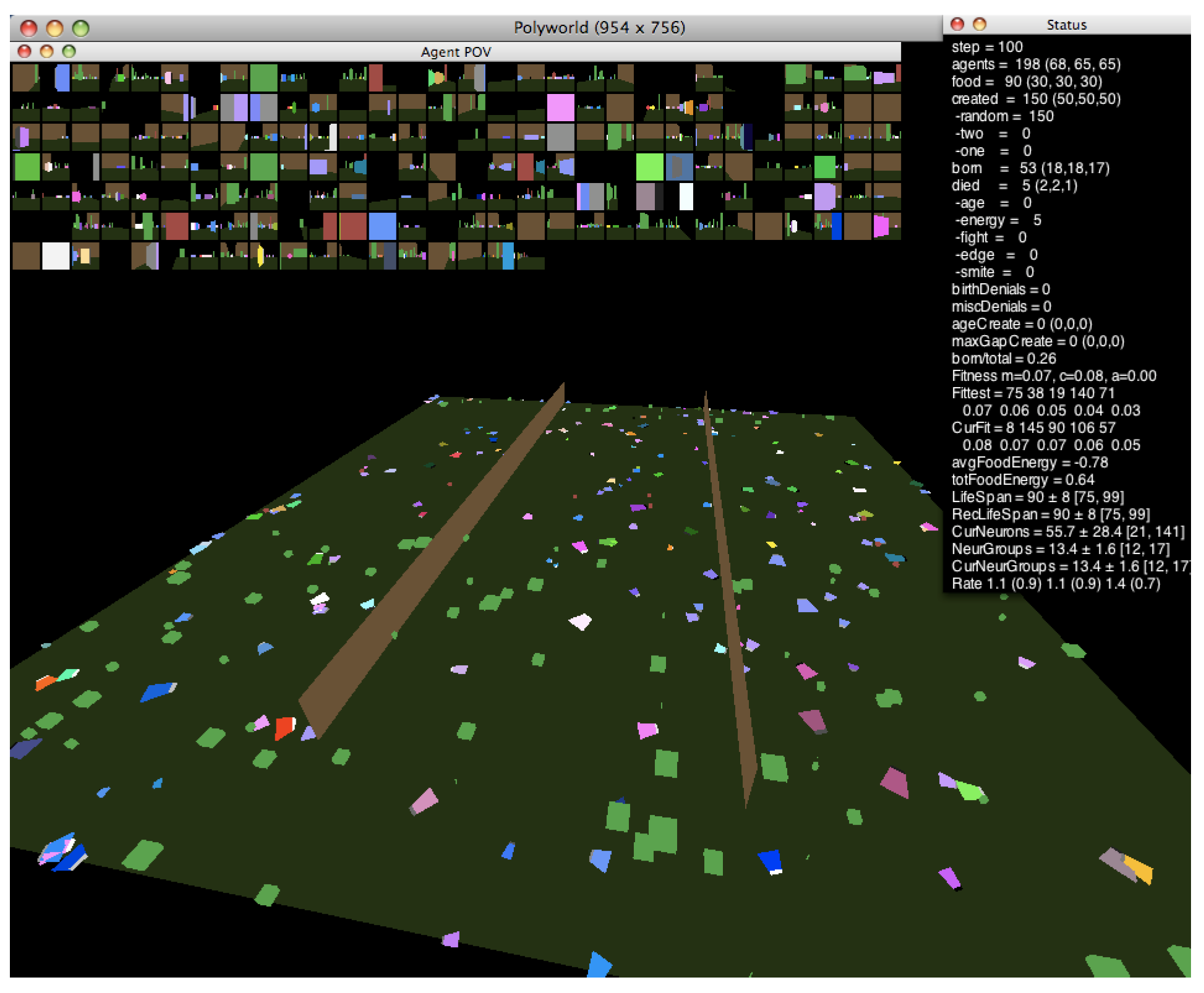
In this work, we investigate the relationship between neural dynamics and the edge of chaos using the agent-based artificial life simulator Polyworld [13]. Shown in Figure 1, Polyworld’s ecology consists of trapezoidal agents and rectangular food items on a flat ground plane that is optionally partitioned into separate regions by vertical barriers. Each agent is controlled by a neural network. The inputs to this network are mainly visual: at each timestep, the environment is rendered from the agent’s point of view (as shown in the small boxes—one for each agent—at the top of Figure 1). The resulting pixels are passed to the network as if they were light falling on a retina. The network’s outputs control the agent’s seven behaviors: move, turn, eat, mate, fight, focus (adjust the agent’s field of view), and light (adjust the brightness of a cluster of polygons on the front of the agent).
Agents expend energy with all actions. In a typical Polyworld simulation, this includes neural activity, but for the experiments discussed here, neural energy costs were disabled to avoid imposing “physical” constraints on network topology. Energy is also lost by coming into contact with an agent that is expressing its fight behavior. An agent may replenish its energy by eating the naturally occurring food items. When its energy is exhausted or when it reaches a genetically specified maximum lifespan, the agent dies.
An agent’s genome specifies characteristics of its physiology and neural structure. Mating between two agents produces a child whose genome is a mutated combination of the two parent genomes. Agents evolve under the influence of natural selection alone; in its standard mode of operation, Polyworld has no fitness function other than survival and reproduction.
Unlike many other artificial life models in which the relationship to biological life is tenuous or purely metaphorical, Polyworld’s motivation is “to create artificial life that is as close as possible to real life, by combining as many critical components of real life as possible in an artificial system” [13]. As such, Polyworld’s design and implementation are heavily biologically inspired—incorporating key elements of natural life—but organized at a high enough level that it is still feasible to simulate and analyze ecology-level dynamics. Compare this to models such as Tierra [14] and Avida [15] in which fragments of computer code are evolved, or to models like Echo [16], where agents’ genetics, physiology, and neural systems are approximated much more coarsely—or not at all. With a level of biological verisimilitude not seen in most other models, Polyworld “may serve as a tool for investigating issues relevant to evolutionary biology, behavioral ecology, ethology, and neurophysiology” [13].
Indeed, since its initial development, Polyworld has been used in a variety of studies that may be considered ethological [13,17,18] or neurophysiological [19,20,21,22], albeit in an artificial context—but why use this context at all? If the goal is to study, say, animal behavior, why not investigate real animals in the natural world? First, it is not always possible to collect the necessary data. As a computer simulation, Polyworld allows virtually any phenomenon of interest to be instrumented in arbitrarily fine detail. Consider the present study, which analyzes detailed neural activity from hundreds of thousands of agents. Carrying out the corresponding study on real animals would, of course, be infeasible. Second, Polyworld allows us to “rewind the tape” of evolution, performing identical experiments with variations in initial conditions or simulation parameters. This is a crucial element of the null reference model described in Section 1.3.1, which allows adaptive evolutionary trends to be recognized.
1.2.1. Behavioral Adaptation
At the beginning of a simulation, Polyworld is populated with a group of seed agents. This population is not viable and must evolve in order to avoid dying out. There is thus significant selection pressure on the agents’ genomes, at least until the population becomes capable of sustaining itself. Populations generally adapt behaviorally to the simple environment used for these experiments within the first five to ten thousand timesteps. After this point, a typical agent exhibits evolutionarily adaptive behaviors such as foraging for food and seeking mates for reproduction. Experiments using more complicated environments have shown that populations are capable of distributing themselves ideally with respect to resources [17] and tracking a moving food patch. (For videos of these and other experiments, see [23].)
1.2.2. Neural Structure
Polyworld’s neural networks (see Figure 2) are separated into five input groups, a variable number of internal groups, and seven output neurons. Three of the input groups provide red, green, and blue color vision, with a variable number of neurons dedicated to each group. The other two input groups consist of single neurons: (1) a neuron that tracks the agent’s current energy level; and (2) a neuron that is activated randomly at each timestep. The seven output neurons correspond to the seven behaviors described in Section 1.2.
An agent’s genome specifies much of its neural structure, including the number of vision neurons dedicated to each color, the number of internal groups, and the number of excitatory and inhibitory neurons within each internal group. Notably, synaptic weights are not stored in the genome. Instead, connections between each pair of groups are described at a relatively high level in the genome using two parameters: connection density (the proportion of possible connections that are actually realized) and topological distortion (the degree to which connections are made randomly rather than sequentially). Synaptic weights are randomized at birth, then updated throughout the agent’s lifetime via a Hebbian learning rule. Weights have a maximum magnitude that is identical for all agents and held constant for the duration of a simulation. Since connections may be excitatory (positive weight) or inhibitory (negative weight), all weights are constrained to the interval .
1.3. Prior Work
1.3.1. Driven and Passive
Much recent work on Polyworld has analyzed the information-theoretic and structural properties of its evolved neural networks [19,20,21,22,24]. Trends toward increased complexity and small-worldness have been observed over evolutionary time. But are these trends actively selected for by evolution, or are they a consequence of the “left wall” of evolutionary simplicity [25]? In other words, the seed population is so simple that it must complexify—there is no room for further simplification. Might the observed trends be explained by a growth in variance coupled with the presence of this lower bound of simplicity?
To answer this question, a null-model (passive) mode of simulation was developed to complement Polyworld’s standard (driven) mode [19]. Here, driven and passive are used in the sense proposed by McShea [26]: the former indicates evolution by natural selection, while the latter indicates a random walk through gene space. In driven mode, a standard simulation is run under the influence of natural selection, during which the birth and death of each agent are recorded. In passive mode, natural births and deaths are disallowed. Instead, these events occur randomly, but in lockstep with the previously completed driven simulation. At each timestep when a birth occurred in the driven simulation, two random agents are mated in the passive simulation; at each timestep when a death occurred in the driven simulation, a random agent is killed in the passive simulation. This results in a pair of simulations—one using natural selection, the other a product of random genetic drift—that are statistically comparable with respect to population.
1.3.2. Numerical Analysis
Qualitatively, driven simulations produce agents that exhibit evolutionarily adaptive behaviors (e.g., foraging and mating), while passive simulations do not. In an effort to quantify this result, early numerical analysis of Polyworld focused on information-theoretic metrics such as entropy, mutual information, integration, and complexity [19,20,24]. Figure 3 shows the average complexity over evolutionary time for ten driven/passive pairs of simulations. The complexity metric used here is related to the interaction complexity of Tononi et al. [27,28], which measures the amount of a system’s entropy that is accounted for by interactions among its elements:
Figure 3 (and similar ones that follow) was generated by binning agents at 1000-timestep intervals based on their time of death. For example, a data point at represents the mean of all agents who died within the first 1000 timesteps. Differences between driven and passive means were assessed for statistical significance using a dependent Student’s t-test, since driven and passive simulations are generated in pairs. Significance is shown by the 1 p-value trend over evolutionary time at the bottom of the figure. High values (exceeding 0.95) indicate a significant difference between the driven and passive simulations (i.e., a selection bias relative to random genetic drift).
Note that complexity initially grows significantly faster in the driven simulations, but only for the first several thousand timesteps. This corresponds roughly to the period of behavioral adaptation—the early portion of the simulation during which agents evolve adaptive behaviors. After this period, driven complexity remains relatively constant or, in a number of cases, even decreases (although some simulations produce a second growth spurt in complexity, as competition between agent subpopulations drives a kind of punctuated equilibrium [18]). Passive complexity, however, continues to grow for an additional 20,000 or so timesteps, ultimately attaining a much higher value, despite the fact that agents in these simulations never evolve adaptive behaviors.
How can we explain this result? Yaeger et al. [19] propose that driven complexity is only correlated with evolutionary fitness during the period of behavioral adaptation. Once a population’s complexity is “good enough” to enable survival, evolution begins to select for stability instead of increasing complexity, since any adaptation away from this “good enough” solution is likely to be detrimental. In Dennett’s words, “the cheapest, least intensively designed system will be ‘discovered’ first by Mother Nature, and myopically selected” [29]. Driven complexity thus stabilizes once the population attains a sufficient fitness. In contrast, since passive simulations are not constrained by natural selection, passive complexity continues to grow—simply as a result of the “left wall” of evolutionary simplicity—until genetic variance is maximized. Complexity is not strictly tied to evolutionary fitness, thus it is unsurprising that passive complexity growth is not accompanied by the evolution of adaptive behaviors.
McShea and Hordijk [30] provide further insight into the possible reasons for the observed complexity trend. On the Darwinian view, complexity evolves monotonically via a process of incremental addition: initially simple structures are steadily enhanced by the addition of new parts through natural selection, with each addition representing a marginal improvement to overall fitness. McShea’s and Hordijk’s alternative view of “complexity by subtraction” proposes that complexity grows early in evolution “perhaps on account of the spontaneous tendency for parts to differentiate” given the system’s initial simplicity. An overproliferation of structures results in a system that is functionally successful yet unstable and inefficient. A reduction in complexity follows, “perhaps driven by selection for effective and efficient function”, which requires simplification following the initially excessive complexity growth. This view provides a possible explanation for the decrease in complexity observed in the later stages of some driven simulations.
More recent numerical analysis of Polyworld using graph-theoretic metrics has produced similar results to those of Figure 3: during the period of behavioral adaptation, driven simulations exhibit a statistically greater tendency toward small-world neural networks. Once the population is capable of sustaining itself, the driven trend plateaus and is surpassed by the passive trend [21]. Thus, our primary interest is in the rate of change of a quantity during the first several thousand timesteps, not in the extremal value it attains later in the simulation.
To summarize, agents in a driven simulation adapt behaviorally to their environment within the first several thousand timesteps, after which the population stabilizes around a “good enough” survival strategy. Since strong selection pressure only exists during this period of behavioral adaptation, it is during this time that we are interested in investigating the effects of evolution. Thus, our question of “Is a particular trend actively selected for by evolution?” becomes “Does the driven trend significantly outpace the passive trend during the period of behavioral adaptation?” Prior work—investigating both information-theoretic [20] and structural [21] metrics of the evolved neural networks—indicates that adaptive trends are significantly faster in driven simulations.
1.4. Our Hypothesis
At this point, we highlight two observations: (1) the edge of chaos seems to facilitate computation; and (2) in Polyworld, natural selection drives adaptive trends significantly faster than a random walk through gene space during the period of behavioral adaptation. Based on these observations, our hypothesis is that agents’ neural dynamics should evolve in the direction of the edge of chaos, and that, during the first several thousand timesteps, this trend should be significantly faster in driven simulations than in passive simulations.
2. Materials and Methods
2.1. Neural Model
Polyworld uses discrete-time firing-rate neural networks with summing-and-squashing neurons. At each timestep, a neuron updates its activation according to
where is the activation of neuron i at time t, is the genetically specified bias of neuron i, is the synaptic weight from neuron j to neuron i at time t, and is a squashing function. We define the normalized synaptic weight as (so that ) and rewrite Equation (2) as
Equation (3) allows us to use as a control parameter in investigating the agents’ neural dynamics. The squashing function used in Polyworld is the logistic curve
where is a globally constant logistic slope. Throughout an agent’s lifetime, its synaptic weights are updated according to the Hebbian learning rule
where is a genetically specified learning rate. The decay function D slowly weakens synapses whose weights have a magnitude greater than :
where r is a globally constant decay rate.
Note that a neuron’s activation is a function of all neurons’ activations in the previous timestep:
Though agents can make use of an input neuron that is activated randomly, Equation (7) itself is deterministic. The network may therefore be viewed as a set of difference equations amenable to dynamical systems analysis.
2.2. “In Vitro” Analysis
Polyworld logs the neural anatomy (i.e., the neural network connection matrix) for each agent at both birth and death. As shown in the following sections, we use a variety of metrics to recognize and quantify chaos “in vitro”: after a simulation has completed, we reconstruct the networks from these log files and analyze their behavior in response to different inputs. In order to more directly extend prior information-theoretic [20] and structural [21] analyses, we use the neural anatomy recorded at death to calculate these metrics. Synaptic weights are held constant during the analysis (i.e., the Hebbian learning rule and decay function of Equation (5) are not applied) so that the analyzed neural anatomy remains exactly the same as the recorded neural anatomy.
Why not perform an “in vivo” analysis? In other words, why not analyze the actual time series of neural activations recorded during agents’ lifetimes? Since our aim is to investigate the edge of chaos, our analysis must allow the manipulation of a control parameter (in this case, ). This is not possible using “in vivo” neural dynamics, as is fixed during a Polyworld simulation. It is thus important to note that the results presented here investigate the dynamics that Polyworld’s neural networks are capable of in general, not the dynamics they happen to exhibit during a simulation.
2.3. Maximal Lyapunov Exponent
Lyapunov exponents measure the average rate at which predictability is lost in a system [1]. The rate of divergence of two initially close trajectories is dominated by the maximal Lyapunov exponent (MLE), defined as
where is the initial separation between the two trajectories and is the separation at time t. The sign of the MLE is indicative of the overall behavior of the system: for , trajectories converge over time, while for , trajectories diverge over time. A positive MLE may thus indicate chaos, although this condition alone is not sufficient to determine whether a system is truly chaotic or merely sensitive to initial conditions. Intuitively, as systems approach the edge of chaos, their MLEs should tend toward zero.
General techniques exist for calculating the MLE from sets of equations [1] and time series [31]. Here, we use a method adapted from Albers et al. [32] that is targeted toward neural networks. First, we iterate the network 100 times using random inputs. This is analogous to showing visual noise to the agent, which moves the network into some random area of its phase space. Next, we iterate the network 1000 times with all inputs set to zero. This is analogous to plunging the agent into total darkness, which allows the network to quiesce toward an attractor.
At this point (), we create a copy of the network, slightly perturb the neural activations, and measure the effect of this perturbation over time. To accomplish this, we take the network’s activations as the vector . We ignore the input neurons, since their activations are completely determined by the agent’s environment. This vector is copied into and displaced by a small with magnitude :
This results in two networks with slightly different activations (conceptually, two trajectories separated by ). Both networks are iterated once with all inputs set to zero, yielding activation vectors and that are separated by
The network’s response to the perturbation can be determined by comparing to . If , the trajectories converged, representing a negative contribution to the MLE. If , the trajectories diverged, representing a positive contribution. Prior to performing the next iteration, is rescaled to the magnitude of the original perturbation:
The copied network’s activations are then reset to so that the trajectories are again separated by (see Figure 4). After iterations, the MLE is estimated as
where indicates the separation between trajectories at time t before rescaling:
2.4. Bifurcation Diagrams
Bifurcation diagrams are used to depict the long-term behavior of a system in response to a varying control parameter [1]. They are generated by selecting a random initial condition and iterating the system a large number of times. The final value of the system is plotted against the value of the control parameter. Many such points are plotted as the parameter is swept through the desired range.
In nonchaotic regimes, the bifurcation diagram collapses to a single point (representing a stable equilibrium) or a set of n points (representing a stable limit cycle of period n). Chaotic regimes appear as widely spread points, indicating the system’s aperiodicity and long-term unpredictability. As with the MLE, this condition is not sufficient to indicate chaos; quasiperiodicity may also appear as widely spread points in a bifurcation diagram.
After Albers et al. [32], we use the maximum synaptic weight as our control parameter. In all the simulations investigated, was fixed at 8. This analysis varies from 0.1 to 50 in increments of 0.1. For each value of , we first iterate the network 100 times with random inputs. Next, we iterate the network 100 times with all inputs set to zero. Finally, we plot the activation of a selected output neuron against the current value of . This procedure is repeated 100 times for each value of , yielding a total of 50,000 points for .
2.5. Onset of Criticality
For different agents, the first appearance of rich dynamics occurs at different values of . We define the onset of criticality (OOC) as the least value of for which the MLE exceeds some threshold. Like the MLE, this metric provides an indication of the level of chaos in the agents’ neural networks. However, unlike the MLE, the OOC takes into account much more of the possible neural dynamics, since it investigates a range of values. Intuitively, if dynamics are being tuned toward the edge of chaos, the OOC should tend toward the actual value of . Note that an MLE of zero is observed at not only transitions to chaos but also, e.g., Hopf bifurcations. The onset of criticality should thus not necessarily be taken as an onset of chaos, but rather as indicating a transition to richer neural dynamics.
Using the method in Section 2.3, we calculate the MLE for each agent while varying from 1 to 100. The OOC is recorded as the least value of for which the MLE exceeds some threshold . We only consider integral values of in order to make this analysis computationally feasible; the fine-grained analysis described in Section 2.4—varying in increments of 0.1—becomes prohibitively time-consuming when applied to ten pairs of simulations, each consisting of tens of thousands of agents. Restricting to integral values is relatively coarse but leads to conservative results since the reported OOC will be no smaller than the actual OOC.
The threshold value must be chosen with care. Even at arbitrarily high values of , some agents’ MLEs remain significantly negative or even undefined. If is chosen too close to zero, these agents’ MLEs will never exceed it. In such cases, the OOC is undefined, and the corresponding agents are excluded from the analysis. However, if is chosen too far from zero (in an attempt to include more agents in the analysis), the OOC will fail to capture its intended meaning. Despite this, the OOC trend appears stable over a range of thresholds. We report here, as this includes the majority (roughly 85%) of all agents.
3. Results
3.1. Maximal Lyapunov Exponent
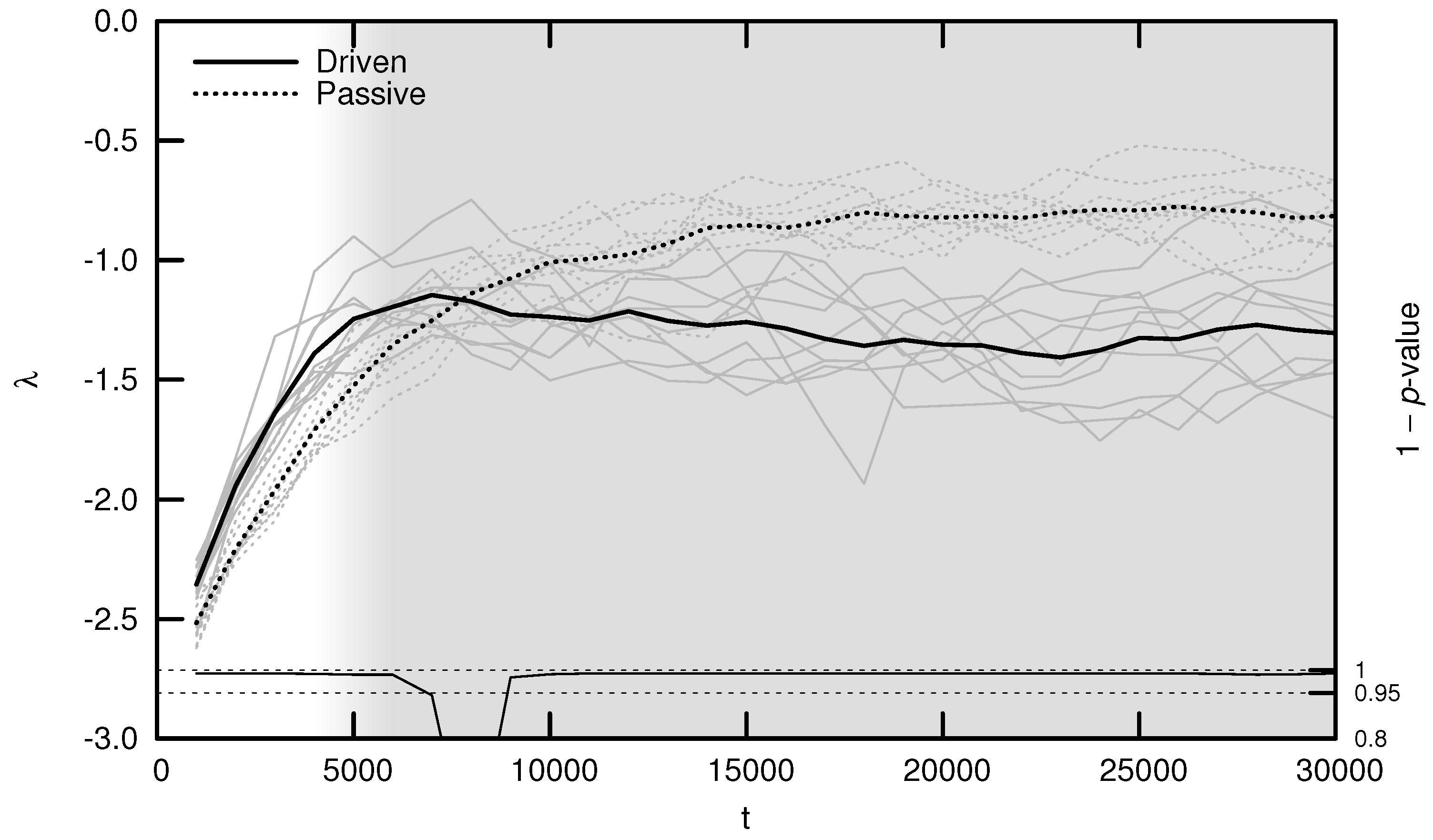
As shown in Figure 5, the average MLE over evolutionary time behaves as predicted: during the period of behavioral adaptation, the driven MLE increases faster than the passive MLE. This difference is statistically significant for the first 6000 timesteps, after which the driven MLE plateaus and is surpassed by the passive MLE. This is the same trend observed for complexity (see Figure 3) and may be explained using similar reasoning: once a population’s neural dynamics are sufficiently rich to implement a “good enough” survival strategy, evolution begins to select for stability. Note, however, that the MLE remains significantly distant from its critical value of zero, indicating that the relatively simple environment used for these experiments may be “solved” using relatively stable neural dynamics.
3.2. Bifurcation Diagrams
Typical bifurcation diagrams are shown in Figure 6, arranged in chronological order of agent death. Each diagram is accompanied by a plot showing the MLE over the same range of values. All agents were taken from a single driven simulation.
Note that these diagrams represent a small fraction of the population for this simulation. We include these results—without comparison to the corresponding passive simulation—for two reasons: (1) to demonstrate the various routes to chaos exhibited by the evolved networks; and (2) to provide context for the results presented in Section 3.3 examining the OOC. While the bifurcation diagrams shown here are helpful in exploring the detailed neural dynamics of individual agents, the OOC is a much more effective metric for meaningfully extrapolating these results to an evolutionary trend.
Agent (a), one of the seed agents of the population, exhibits virtually no change in neural dynamics for varying . Agent (b) is typical of agents that have evolved marginally from this seed population: varying induces a monotonic increase or decrease in neural activation, but there is no evidence of chaotic behavior (indeed, for both agents (a) and (b), the MLE is undefined, indicating that these agents’ networks do not respond to perturbation). Agent (c) exhibits richer dynamics at relatively high values of . This regime tends to expand and move leftward toward over evolutionary time, as seen in agents (d) through (g). Evidence of period-doubling bifurcations and quasiperiodicity can be seen in agents (e) and (f). Agent (g) appears to be tuned precisely to critical behavior: the MLE approaches zero precisely at . Agent (h) is an example of an agent tuned past this critical point, with chaotic behavior evident at .
3.3. Onset of Criticality
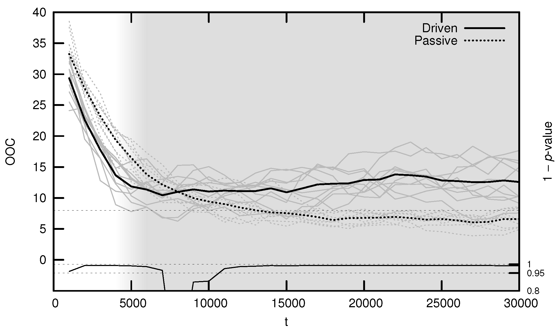
The average OOC over evolutionary time is shown in Figure 7. The approach toward is significantly faster in the driven simulations during the period of behavioral adaptation. As with the MLE, the driven OOC plateaus after this period, remaining somewhat distant from its critical value.
4. Discussion
Polyworld’s evolved neural networks are driven in the direction of the edge of chaos. There are two main pieces of evidence for this claim: over evolutionary time, (1) the average MLE increases toward zero; and (2) the average onset of criticality decreases toward the actual maximum synaptic weight . During the period of behavioral adaptation to the environment, these trends are significantly faster when driven by natural selection than in a random walk through gene space. Both of the metrics studied remain distant from their critical values, but this is unsurprising: previous work indicates that once a “good enough” survival strategy is found, evolution begins to select for stability.
Future work could supplement these results by addressing a number of questions. How does the MLE change as a function of distance in parameter space from evolved network parameters? What is the distribution of MLEs for networks generated randomly within this space? How are neural dynamics related to adaptive behavior? For example, are agents at the edge of chaos more likely to exhibit behaviors such as foraging and mating? How much of a role do developmental changes (via Hebbian learning) play in the trends we observe over evolutionary time? What correlations are there between the metrics discussed here and the previously investigated information- and graph-theoretic metrics?
This work could also motivate some modifications to Polyworld. For instance, rather than using a fixed , this quantity could be pushed into the agents’ genomes, allowing a population to evolve its value in concert with their neural topologies.
Supplementary Materials
The source code for Polyworld is available online at https://github.com/polyworld/polyworld.
Acknowledgments
This work was supported by the National Academies Keck Futures Initiative Grant No. NAKFI CS22 and by the National Science Foundation Integrative Graduate Education and Research Traineeship award number 0903495.
Author Contributions
Larry Yaeger developed Polyworld. Steven Williams performed the analysis. Both authors designed the experiment and contributed to writing the paper.
Conflicts of Interest
The authors declare no conflict of interest.
References
- Sprott, J.C. Chaos and Time-Series Analysis; Oxford University Press: Oxford, UK, 2003. [Google Scholar]
- Langton, C.G. Computation at the Edge of Chaos: Phase Transitions and Emergent Computation. Physica D 1990, 42, 12–37. [Google Scholar] [CrossRef]
- Bornholdt, S.; Röhl, T. Self-organized critical neural networks. Phys. Rev. E 2003, 67, 066118. [Google Scholar] [CrossRef] [PubMed]
- Bertschinger, N.; Natschläger, T. Real-Time Computation at the Edge of Chaos in Recurrent Neural Networks. Neural Comput. 2004, 16, 1413–1436. [Google Scholar] [CrossRef] [PubMed]
- Skarda, C.A.; Freeman, W.J. How brains make chaos in order to make sense of the world. Behav. Brain Sci. 1987, 10, 161–195. [Google Scholar] [CrossRef]
- Goldberger, A.L.; Rigney, D.R.; West, B.J. Chaos and Fractals in Human Physiology. Sci. Am. 1990, 262, 42–49. [Google Scholar] [CrossRef] [PubMed]
- Schiff, S.J.; Jerger, K.; Duong, D.H.; Change, T.; Spano, M.L.; Ditto, W.L. Controlling chaos in the brain. Nature 1994, 370, 615–620. [Google Scholar] [CrossRef] [PubMed]
- Boedecker, J.; Obst, O.; Lizier, J.T.; Mayer, N.M.; Asada, M. Information processing in echo state networks at the edge of chaos. Theory Biosci. 2012, 131, 205–213. [Google Scholar] [CrossRef] [PubMed]
- Goudarzi, A.; Teuscher, C.; Gulbahce, N.; Rohlf, T. Emergent Criticality Through Adaptive Information Processing in Boolean Networks. Phys. Rev. Lett. 2012, 108, 128702. [Google Scholar] [CrossRef] [PubMed]
- Lizier, J.T.; Prokopenko, M.; Zomaya, A.Y. The Information Dynamics of Phase Transitions in Random Boolean Networks. Artif. Life 2008, 11, 374–381. [Google Scholar]
- Mitchell, M.; Hraber, P.T.; Crutchfield, J.P. Revisiting the Edge of Chaos: Evolving Cellular Automata to Perform Computations. Complex Syst. 1993, 7, 89–130. [Google Scholar]
- Snyder, D.; Goudarzi, A.; Teuscher, C. Finding Optimal Random Boolean Networks for Reservoir Computing. Artif. Life 2012, 13, 259–266. [Google Scholar]
- Yaeger, L. Computational Genetics, Physiology, Metabolism, Neural Systems, Learning, Vision, and Behavior or PolyWorld: Life in a New Context; Langton, C.G., Ed.; Artificial Life III; Santa Fe Institute: Santa Fe, NM, USA, 1994; pp. 263–298. [Google Scholar]
- Ray, T.S. An Approach to the Synthesis of Life; Langton, C.G., Taylor, C., Farmer, J.D., Rasmussen, S., Eds.; Artificial Life II; Oxford University Press: Oxford, UK, 1992; pp. 371–408. [Google Scholar]
- Adami, C.; Brown, C.T. Evolutionary Learning in the 2D Artificial Life System “Avida”; Brooks, R.A., Maes, P., Eds.; Artificial Life IV; MIT Press: Cambridge, MA, USA, 1994; pp. 377–381. [Google Scholar]
- Holland, J.H. Hidden Order: How Adaptation Builds Complexity; Basic Books: New York, NY, USA, 1995. [Google Scholar]
- Griffith, V.; Yaeger, L.S. Ideal Free Distribution in Agents with Evolved Neural Architectures. In Artificial Life X: Proceedings of the Tenth International Conference on the Simulation and Synthesis of Living Systems, Bloomington, IN, USA, 3–6 June 2006; Rocha, L.M., Ed.; MIT Press: Cambridge, MA, USA, 2006; pp. 372–378. [Google Scholar]
- Murdock, J.; Yaeger, L.S. Identifying Species by Genetic Clustering; Lenaerts, T., Ed.; Advances in Artificial Life, ECAL 2011; Indiana University: Bloomington, IN, USA, 2011; pp. 564–572. [Google Scholar]
- Yaeger, L.; Griffith, V.; Sporns, O. Passive and Driven Trends in the Evolution of Complexity; Bullock, S., Noble, J., Watson, R., Bedau, M.A., Eds.; Artificial Life XI; MIT Press: Cambridge, MA, USA, 2008; pp. 725–732. [Google Scholar]
- Yaeger, L.S. How evolution guides complexity. HFSP J. 2009, 3, 328–339. [Google Scholar] [CrossRef] [PubMed]
- Yaeger, L.; Sporns, O.; Williams, S.; Shuai, X.; Dougherty, S. Evolutionary Selection of Network Structure and Function. In Artificial Life XII, Proceedings of the 12th International Conference on the Synthesis and Simulation of Living Systems, Odense, Denmark, 19–23 August 2010; Fellermann, H., Dorr, M., Hanczyc, M.M., Laursen, L.L., Maurer, S., Merkle, D., Monnard, P.A., Stoy, K., Rasmussen, S., Eds.; MIT Press: Cambridge, MA, USA, 2010; pp. 313–320. [Google Scholar]
- Lizier, J.T.; Piraveenan, M.; Pradhana, D.; Prokopenko, M.; Yaeger, L.S. Functional and Structural Topologies in Evolved Neural Networks. Adv. Artif. Life 2011, 5777, 140–147. [Google Scholar]
- Yaeger, L. Polyworld Movies. Available online: http://shinyverse.org/larryy/PolyworldMovies.html (accessed on 4 July 2017).
- Yaeger, L.S.; Sporns, O. Evolution of Neural Structure and Complexity in a Computational Ecology. In Artificial Life X: Proceedings of the Tenth International Conference on the Simulation and Synthesis of Living Systems, Bloomington, IN, USA, 3–6 June 2006; Rocha, L.M., Ed.; MIT Press: Cambridge, MA, USA, 2006; pp. 372–378. [Google Scholar]
- Gould, S.J. The Evolution of Life on the Earth. Sci. Am. 1994, 271, 85–91. [Google Scholar] [CrossRef]
- McShea, D.W. Metazoan Complexity and Evolution: Is There a Trend? Int. J. Org. Evol. 1996, 50, 477–492. [Google Scholar]
- Tononi, G.; Sporns, O.; Edelman, G.M. A measure for brain complexity: Relating functional segregation and integration in the nervous system. Proc. Natl. Acad. Sci. USA 1994, 91, 5033–5037. [Google Scholar] [CrossRef] [PubMed]
- Tononi, G.; Edelman, G.M.; Sporns, O. Complexity and coherency: integrating information in the brain. Trends Cogn. Sci. 1998, 2, 474–484. [Google Scholar] [CrossRef]
- Dennett, D.C. Kinds of Minds: Toward an Understanding of Consciousness; Basic Books: New York, NY, USA, 1996. [Google Scholar]
- McShea, D.W.; Hordijk, W. Complexity by Subtraction. Evol. Biol. 2013, 40, 504–520. [Google Scholar] [CrossRef]
- Wolf, A.; Swift, J.B.; Swinney, H.L.; Vastano, J.A. Determining Lyapunov Exponents from a Time Series. Physics D 1985, 16, 285–317. [Google Scholar] [CrossRef]
- Albers, D.J.; Sprott, J.C.; Dechert, W.D. Routes to Chaos in Neural Networks with Random Weights. Int. J. Bifurc. Chaos 1998, 8, 1463–1478. [Google Scholar] [CrossRef]
Figure 1.
A Polyworld simulation.

Figure 2.
A possible neural structure of a Polyworld agent. Input groups project to internal and output groups. Internal and output groups project to each other and recurrently to themselves. Only representative connections are shown; those involving internal groups other than the large central group are mostly suppressed.
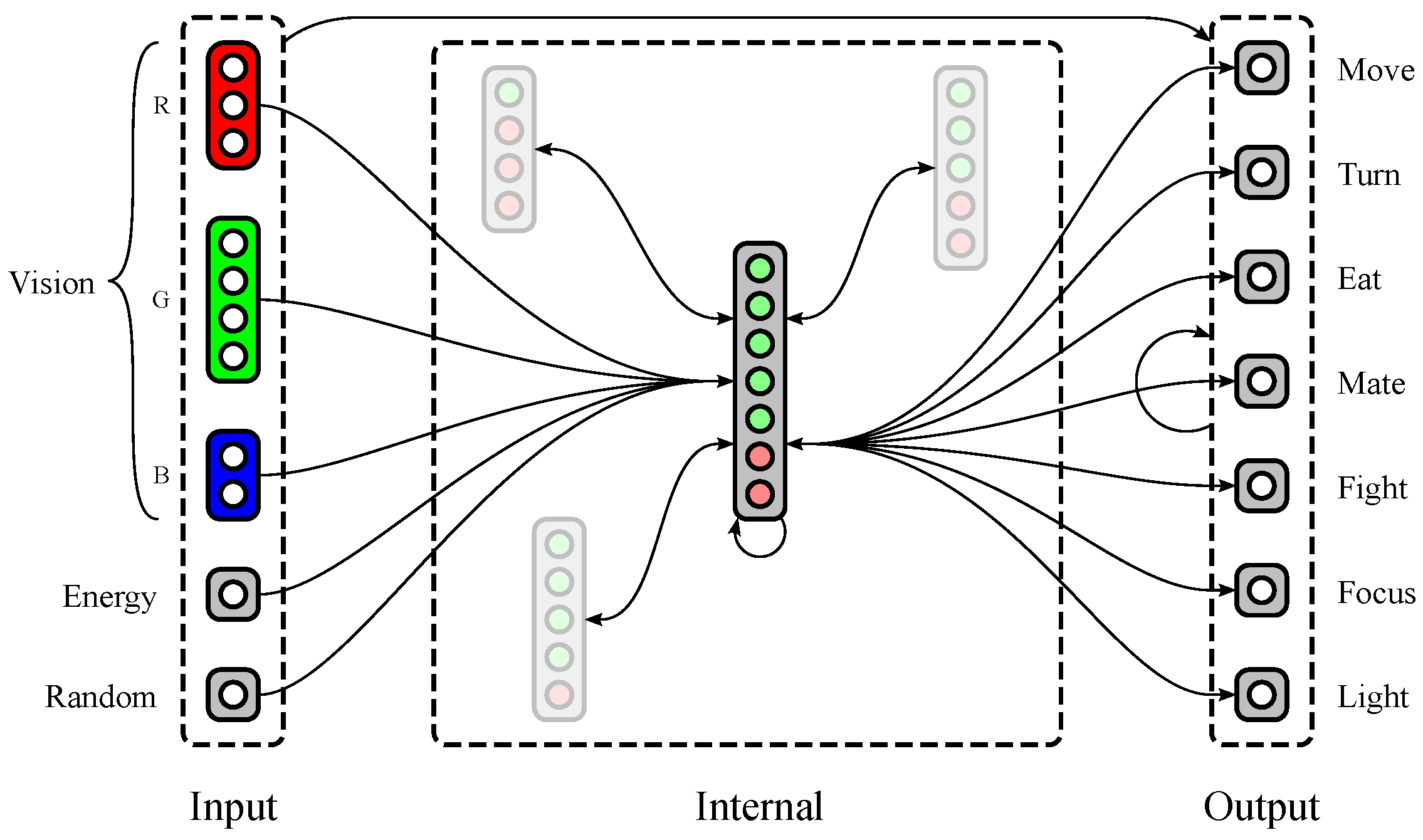
Figure 3.
Average complexity C over evolutionary time t for ten driven/passive pairs of simulations. Light lines show the population-mean complexity for individual simulations, while heavy lines show meta-means over all ten simulations. Statistical significance is indicated by the line at the bottom of the figure, representing 1 p-value for a dependent Student’s t-test. Reproduced from Yaeger [20].
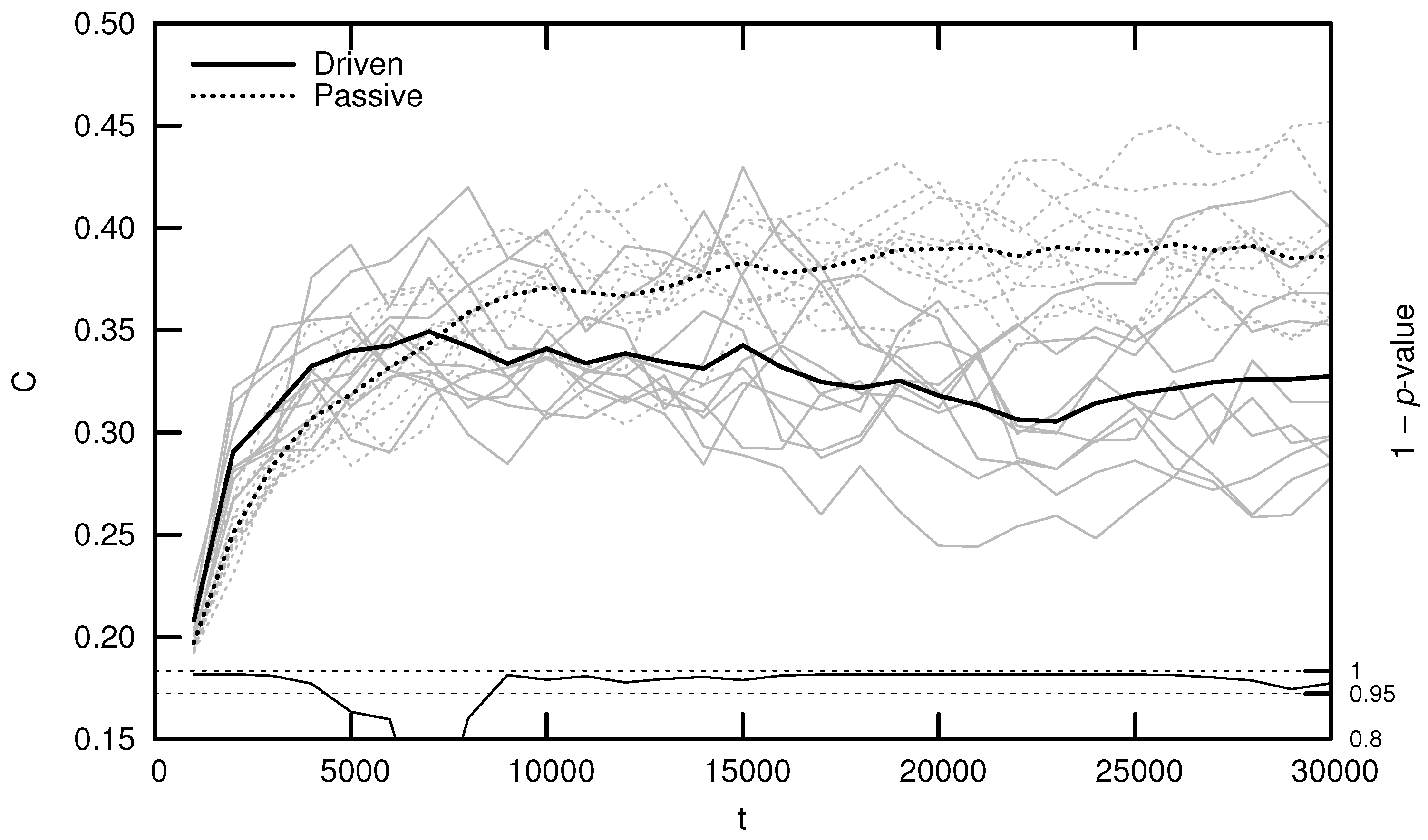
Figure 4.
Calculation of the maximal Lyapunov exponent. Adapted from Boedecker et al. [8].
Figure 4.
Calculation of the maximal Lyapunov exponent. Adapted from Boedecker et al. [8].
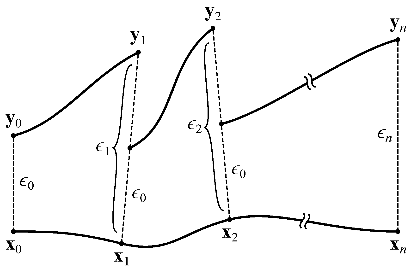
Figure 5.
Average maximal Lyapunov exponent (MLE) over evolutionary time t for ten driven/passive pairs of simulations. Light lines show the population-mean MLE for individual simulations, while heavy lines show meta-means over all ten simulations. Statistical significance is indicated by the line at the bottom of the figure, representing 1 p-value for a dependent Student’s t-test. Shading emphasizes the period of behavioral adaptation ().

Figure 6.
Bifurcation diagrams and maximal Lyapunov exponents for eight different agents in a driven simulation. The dashed vertical line denotes the actual maximum synaptic weight used in the simulation. Diagrams are shown in chronological order, with t indicating the timestep of the agent’s death.
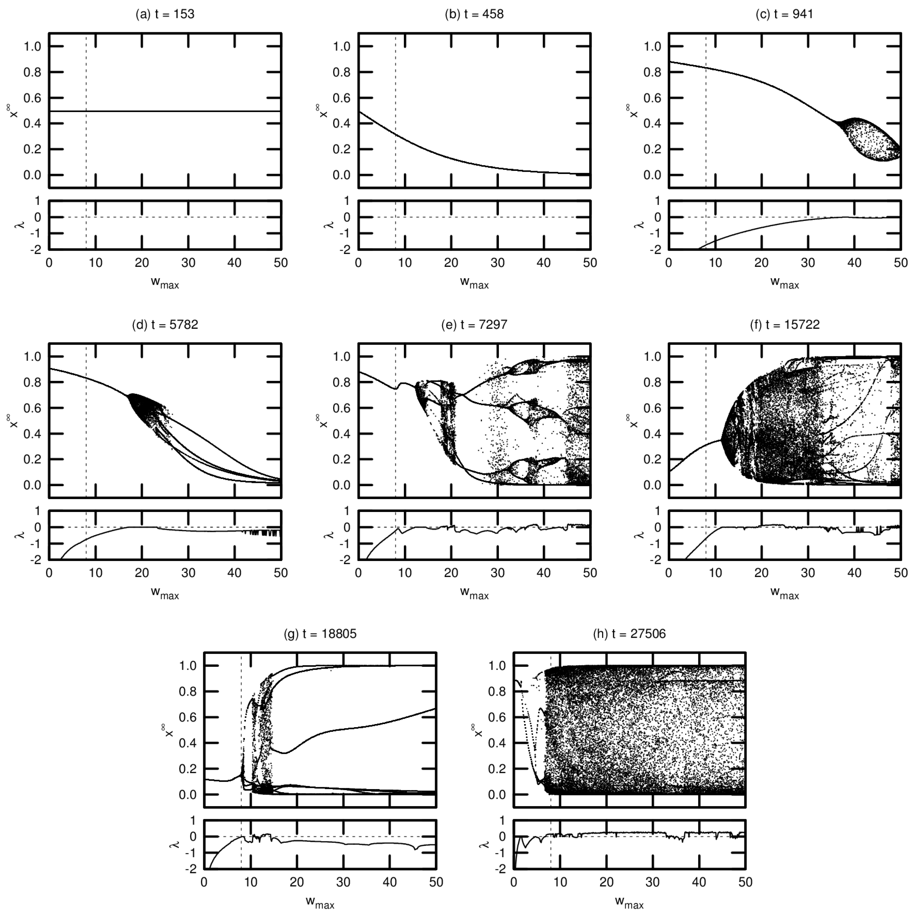
Figure 7.
Average onset of criticality (OOC) over evolutionary time for ten driven/passive pairs of simulations. Light lines show the population-mean OOC for individual simulations, while heavy lines show meta-means over all ten simulations. The dashed horizontal line denotes the actual maximum synaptic weight used in the simulations. Statistical significance is indicated by the line at the bottom of the figure, representing 1 p-value for a dependent Student’s t-test. Shading emphasizes the period of behavioral adaptation ().

© 2017 by the authors. Licensee MDPI, Basel, Switzerland. This article is an open access article distributed under the terms and conditions of the Creative Commons Attribution (CC BY) license (http://creativecommons.org/licenses/by/4.0/).
Share and Cite
MDPI and ACS Style
Williams, S.; Yaeger, L. Evolution of Neural Dynamics in an Ecological Model. Geosciences 2017, 7, 49. https://doi.org/10.3390/geosciences7030049
AMA Style
Williams S, Yaeger L. Evolution of Neural Dynamics in an Ecological Model. Geosciences. 2017; 7(3):49. https://doi.org/10.3390/geosciences7030049
Chicago/Turabian StyleWilliams, Steven, and Larry Yaeger. 2017. "Evolution of Neural Dynamics in an Ecological Model" Geosciences 7, no. 3: 49. https://doi.org/10.3390/geosciences7030049
Note that from the first issue of 2016, this journal uses article numbers instead of page numbers. See further details here.