Investigating the Apparent Seismic Diffusivity of Near-Receiver Geology at Mount St. Helens Volcano, USA

1
Department of Earth Sciences, University of Turin, Via Tommaso Valperga Caluso, 35, 10125 Turin, Italy
2
School of Earth and Environmental Sciences, University of Portsmouth, Burnaby Building, Burnaby Road, Portsmouth PO1 3QL, UK
3
Department of Geology and Petroleum Geology, School of Geosciences, University of Aberdeen, King’s College, Aberdeen AB24 3FX, UK
*
Author to whom correspondence should be addressed.
Geosciences 2017, 7(4), 130; https://doi.org/10.3390/geosciences7040130
Submission received: 16 October 2017
/
Revised: 27 November 2017
/
Accepted: 7 December 2017
/
Published: 15 December 2017
(This article belongs to the Special Issue Volcano Monitoring – Placing the Finger on the Pulse)
Abstract
:We present an expanded approach of the diffusive approximation to map strongly scattering geological structures in volcanic environments using seismic coda intensities and a diffusive approximation. Seismic data from a remarkably consistent hydrothermal source of Long-Period (LP) earthquakes, that was active during the late 2004 portion of the 2004–2008 dome building eruption of Mount St. Helens Volcano, are used to obtain coefficient values for diffusion and attenuation, and describe the rate at which seismic energy radiates into the surrounding medium. The results are then spatially plotted as a function of near-receiver geology to generate maps of near-surface geological and geophysical features. They indicate that the diffusion coefficient is a marker of the near-receiver geology, while the attenuation coefficients are sensitive to deeper volcanic structures. As previously observed by other studies, two main scattering regimes affect the coda envelopes: a diffusive, multiple-scattering regime close to the volcanic edifice and a much weaker, single-to-multiple scattering regime at higher source-receiver offsets. Within the diffusive, multiple-scattering regime, the spatial variations of the diffusion coefficient are sufficiently robust to show the features of laterally-extended, coherent, shallow geological structures.

1. Introduction
Reflection (or scattering) at an acoustic impedance surface is a principal process by which seismic energy propagates through the subsurface. Interfaces characterised by higher impedance contrasts will reflect more energy. In the framework of ray theory, the seismic source, the path the ray takes through the subsurface to the receiver, and the near-surface geology close to the receiver all contribute to energy propagation. While the separation of source and path effects is an extensively studied problem, receiver (or site) effects are often underestimated [1]; however, these effects make a significant contribution to the waveform [2] and, especially in volcanic environments, they may introduce errors into models and interpretations [3,4]. This study links these site effects with the near-receiver geological characteristics, with the aim of discovering if seismic coda wave sensitivities are able to define shallow geological structures.
Given sufficient lapse-time from an initial P-arrival, a coda wave may be considered as a sequence of arrivals of reflected energy from the numerous heterogeneities encountered from source to receiver [5,6]. The amplitude of these arrivals were found to be very similar at different stations for the same event, regardless of distance from the source. What does vary, however, is the length of the coda. This forms the basis of the S-wave coda normalisation method (e.g., Aki 1980 [6]) and a theoretical basis to perform scattering tomography. By normalising the amplitude spectra at a given lapse time, energy is assumed to be uniform around the source at this point, allowing heterogeneities to be mapped spatially using a single-scattering assumption. The key assumption is that, at shallow depths, smaller-scale structures dominate over larger-scale variations, so much so that each arrival seen in the coda is less a function of a single reflection, and more a result (superposition) of multiple scattering events [7].
These shallow effects are especially relevant when studying volcanoes, such as Mount St. Helens (MSH). The geology of this stratovolcano is complicated since it is the result of thousands of years of eruptions and landslides. Such complex geology results in a highly inhomogeneous medium, which then causes significant multiple scattering events as seismic energy propagates through it. By treating the entirety of the volcanic structure as a region of strongly scattering material, it can be assumed that, due to the stochastic nature of the medium, any seismic energy passing through will behave in a diffusive manner [8,9]. By modelling seismic arrivals as the forefront of a diffusive “cloud” of seismic energy, the decay of the P and S energy is heavily affected by the strongly scattering structure close to the seismic receiver.
Wegler (2001 [8] and 2003 [9]) argued that traditional seismic travel time tomography was not good enough to model the expected complexity of a volcanic interior. Hence, they developed the concept of multiple scattering in order to image small-scale heterogeneities. Using the assumption that a volcano can be described as a diffusive regime, the authors considered the decay of the seismic coda to obtain coefficient values for the diffusion and attenuation of seismic energy using an active source experiment at Merapi and Vesuvius volcanoes.
The coefficient values obtained with a diffusive approximation describe the way in which energy is scattered around a medium; the way in which this energy is dispersed changes depending on different lithological properties, even inside the same rock matrix. Figure 1 shows a cartoon representation of scattering behaviour for two different types of media. In panel 1a, a loosely consolidated structure results in very strong scattering of the propagating energy. On the other hand, panel 1b, shows how a small contrast between the acoustical properties of different crystals leads to very weak scattering behaviour. These processes are, evidently, frequency dependent.
Attenuation can be considered a conductive process, where energy is transferred via physical contact rather than through radiative processes [10]. As the seismic wavefield passes through a medium, energy is lost due to conversion to kinetic energy, via elastic perturbations of structural features such as sedimentary grains, or to thermal energy, due to friction between adjacent particles. How quickly energy is attenuated can be seen as a function of how much individual grains can move. In geological terms, freshly deposited sandstone, which is poorly consolidated, will attenuate seismic energy quicker than a much more consolidated, or even crystalline, rock. The presence of fluids may additionally enhance attenuation due to the loss of shear energy.
Diffusion can be described as a result of the spaces between the grains [11]. As a process it is similar to seismic reflection. Energy is reflected off the sides of grains due to high acoustic impedances. The more of these high acoustic impedance surfaces there are, the more the seismic energy is ‘scattered’ around the medium. Some energy is lost at each scatterer due to transmission, but to a far lower degree as compared with the attenuation coefficient. For a review of how seismic diffusion and attenuation can be measured and behave in rock samples we refer to Mavko et al. (2009) [11].
By treating the diffusion and attenuation coefficients together as descriptors of the rate at which energy is lost in the medium, we can describe the geology in terms of consolidation and ability to attenuate energy. Attenuation is conceptually a simple process: higher coefficient values mean higher rates of attenuation and vice versa. The diffusion coefficient meanwhile, is closer to the inverse of ‘scattering’. A lower diffusion value shows that energy is not leaving the local medium—just being constantly scattered around locally. Both are difficult to measure in the field but have wide implications for geophysical imaging in volcanoes [12,13].
This assumption forms the basis of a new way of using the diffusive approximation to depict surface geology, as presented in this paper. By applying the method of Wegler (2003) [9], we process a unique seismic dataset from the late 2004 portion of the 2004–2008 dome building eruption of MSH. The subsequent results are then compared and contrasted to the known near-surface geological structure as documented in the literature.
2. Mount St. Helens Volcano, USA: Geological and Seismic Structure
Mount St. Helens Volcano (MSH) is a region of diverse and complex geology, and one of several active volcanoes located in the Cascade Volcanic Arc of North America. The volcanoes in this area, and particularly MSH, have been extensively studied due to the potential hazard they pose on the metropolitan areas nearby and the destructive potential of their explosive eruptions. Significant volcanism in the region started around 37 million years ago [14] due to the subduction of the Juan de Fuca plate beneath the North American Plate, in a region known today as the Cascadia Subduction Zone. This process has resulted in a complicated network of stratovolcanoes, linked by intrusive bodies and interacting with a diverse range of hydrothermal fluids and partial melt that reach the shallow crust [15,16].
Due to the complex geological structure of the volcanic edifice and plumbing systems at MSH, the two broad scattering regimes identified in Wegler and Lühr (2001) [8] can be observed at the volcano using passive seismicity. Firstly, type A events, located at some distance from the edifice (typically greater than 10 km) and in the frequency range of 5–15 Hz [12]. Secondly, type B events, which originate from within the volcanic edifice itself, and are of lower frequency, generally between 1 Hz and 5 Hz [15,17]. These differences are dependent on both the source dynamics and media properties close to the source [12,13,15]: whilst type A events show clear P- and S-wave arrivals, type B do not show a clear S arrival. Since S-waves do not propagate through fluids this suggests that they are present close to the source of type B events, that is, fluid and molten materials are responsible for their generation [15]. Here, we focus on the near-receiver effects affecting coda waves, that is, those created by strong near-receiver scattering, observed by De Siena et al. (2014) [12]. Using type B events, the authors observe high scattering and high attenuation anomalies up to 6 km depth, indicative of fluid-rich zones within the volcanic plumbing system during the last eruption of the volcano. Kiser et al. (2016) [16] confirmed these results using travel-time velocity tomography.
Far from the source, path effects are primarily manifested in P-wave velocity models as high or low velocity anomalies. Lees (1992) [18] applies P-wave tomography (e.g., Nolet 1987 [19]) to Mount. St. Helens data recorded before and after its main eruption (1980) using a non-linear inversion method of hypocentral relocation and velocity recovery. His purpose was to try to determine the extent of magmatic bodies beneath the volcano, i.e., regions of low velocity, which can be attributed to regions of partial melt occurring in patches. The results show a ~1.5 km deep high-velocity zone, beneath the crater floor interpreted as a volcanic plug, directly above a low-velocity zone—interpreted as the magma conduit. This conduit broadens into a “chamber”, which extends down to around 7.5 km depth. Beneath this region, data coverage was poor, but a second chamber was inferred to exist between 9 and 16 km depth by the same author.
Building on these results and adding seismicity recorded around the 2004 eruption, Waite and Moran (2009) [20] further improve the resolution in the upper 10 km of the crust. They found two igneous intrusive bodies NE and NW of the edifice as well as a structural boundary that runs parallel to the St. Helens Seismic zone (SHZ). These structures had already been retrieved by Moran et al. (1999) [17] and interpreted as a significant NNW trending structural anomaly, which ties in with the regional plate tectonics of a converging plate margin. The main difference between the Lees (1992) [18] and Waite and Moran (2009) [20] models is the location of a high-velocity anomaly. between depths of 3.5 km and 6.5 km. Waite and Moran (2009) [20] showed that this high-velocity body is 1 km deeper and ~1 km further to the east with respect to that of Lees (1992) [18]. Whilst this may seem trivial, it does bring up implications for the interpretation of the extent of magmatic material associated with the seismicity in this region. This difference could be explained by the differences in the techniques used by the different authors, which is largely a matter of advancements in geophysics made in the last 25 years.
Recent velocity imaging from active surveys shows the most up to date picture of the plumbing system of the volcano [15]. By utilising active source data from the iMUSH experiment, a low-Vp columnar anomaly was observed beneath and to the south-east of an inferred magma sill extending to 40 km depth [16]. At the boundary of this region, deep long period seismicity is attributed to the injection of magmatic fluids into the crust. High-density accumulates, which may have a magmatic origin, are also observed and are thought to play an important role in the transport of such fluids within the crust. The low-velocity vertical anomaly gently dips towards SE; a low-scattering, high-intrinsic scattering anomaly retrieved at ~10 km depth by scattering tomography [12]; an high-conductivity anomaly retrieved by means of magnetotelluric tomography and interpreted as an extended crustal magma sill [21]; and a deep low-velocity anomaly, obtained using full-waveform tomography and interpreted as the shallowest extension of a mantle wedge [22].
Even though the geology close to the receivers has the obvious advantage of a visible surface exposure, the effects of the uppermost edifice on a seismic trace are very poorly constrained. Figure 2 shows a simplified geological map, which divides the area into 2 regions. Firstly, a younger, loosely consolidated group of Pleistocene-age volcanic rocks and debris flows. Secondly, an older, much more consolidated region of Oligocene–Miocene deposits. Overlain onto this map is the shallow subsurface extent of the Spud Mountain and Spirit Lake Plutons, along with a third body to the south, which is thought to be part of the Spirit Lake Pluton [23]. Also shown is the extent of the 1980s debris flows, including some of the youngest deposits in this region, which likely show the least amount of consolidation. Poppeliers (2015) [24] demonstrated how a changing consolidation close to receivers has a disproportionally strong effect on the final waveform. By considering the partitioning of strain energy between P and S waves, it was found that sites with a pronounced stratification (layering), in particular, showed a strong frequency dependence on the ratios between direct energy and coda values.
3. Data and Method
3.1. “Drumbeat” Seismicity
Long-period (LP) earthquakes play a key role for driving main eruptions at Mount St. Helens. The 18 May 1980 eruption was preceded by the occurrence of two swarms of low-frequency seismic events and high values of the harmonic tremor indicated the action of interior pressurization promoting the weakening of the volcanic edifice [26].
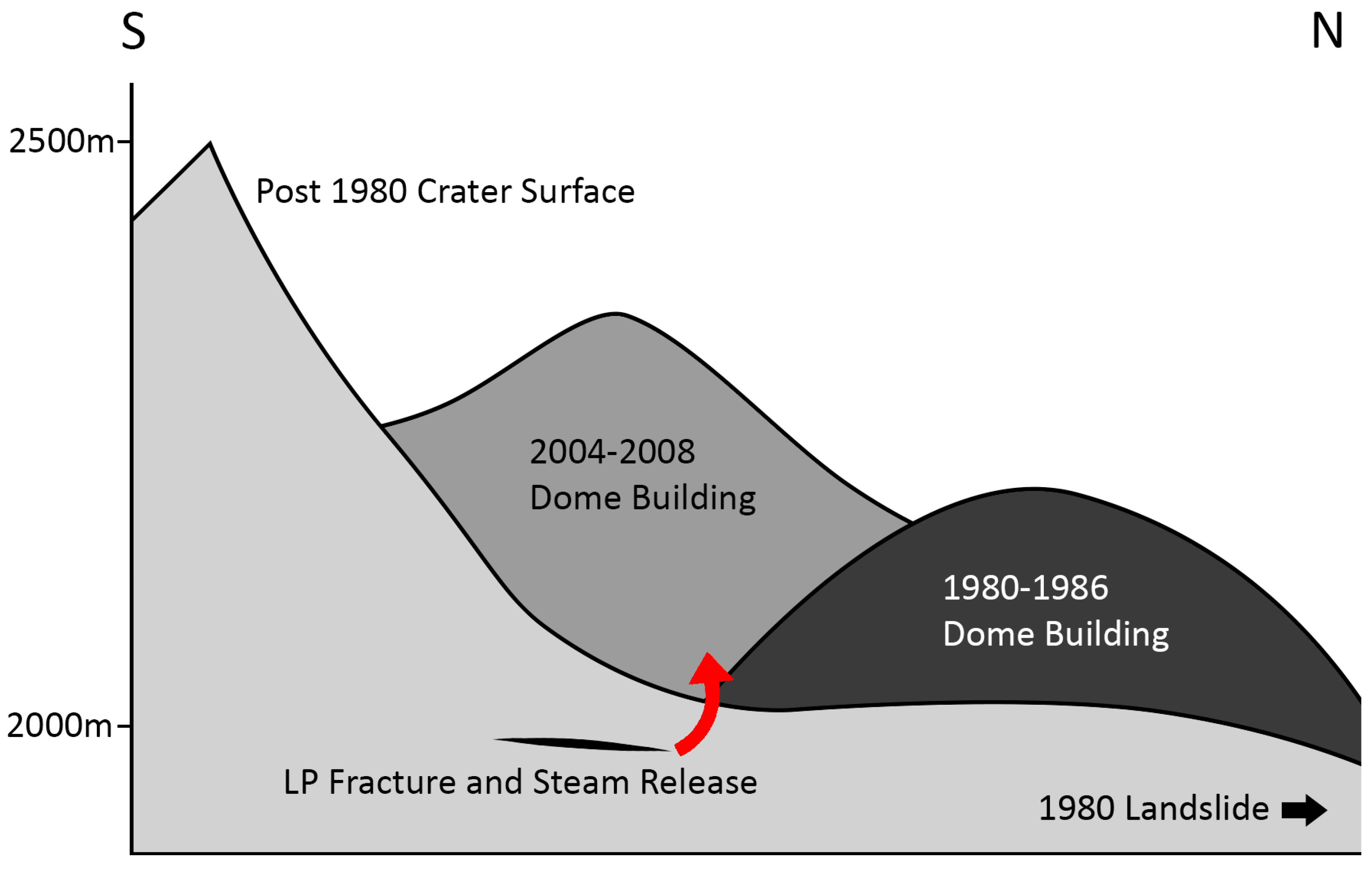
Repetitive and shallow LP earthquakes were extensively recorded during the 2004 MSH eruption and quickly became known as ‘drumbeats’. Although initially attributed to the large amounts of dome building occurring on MSH at the time—structurally manifested as a vertical strike-slip system [27]—the suggested mechanism for generating these ‘drumbeat’ events was that of volumetric changes within a fluid-filled crack/conduit system. Waite et al. (2008) [15] showed how the first motions seen on the observed seismic data are dilatational (and so cannot be part of a strike-slip system) and originate beneath the dome itself at around 2000 m elevation. The actual ‘crack’ itself can be thought of as a fluid-filled fracture between two old lava flows. The LP events are then likely to be generated when magmatic activity below causes the pressure to rise within the fracture; once this increases past a threshold dictated by the frictional forces present, fluid then escapes, generating a characteristic LP event (drumbeat) and also allowing the crack to close [27]. The crack then refills with more fluid and the process repeats itself. Figure 3 is a schematic illustration of the geometry of the source location, modified from previous studies [15,28].
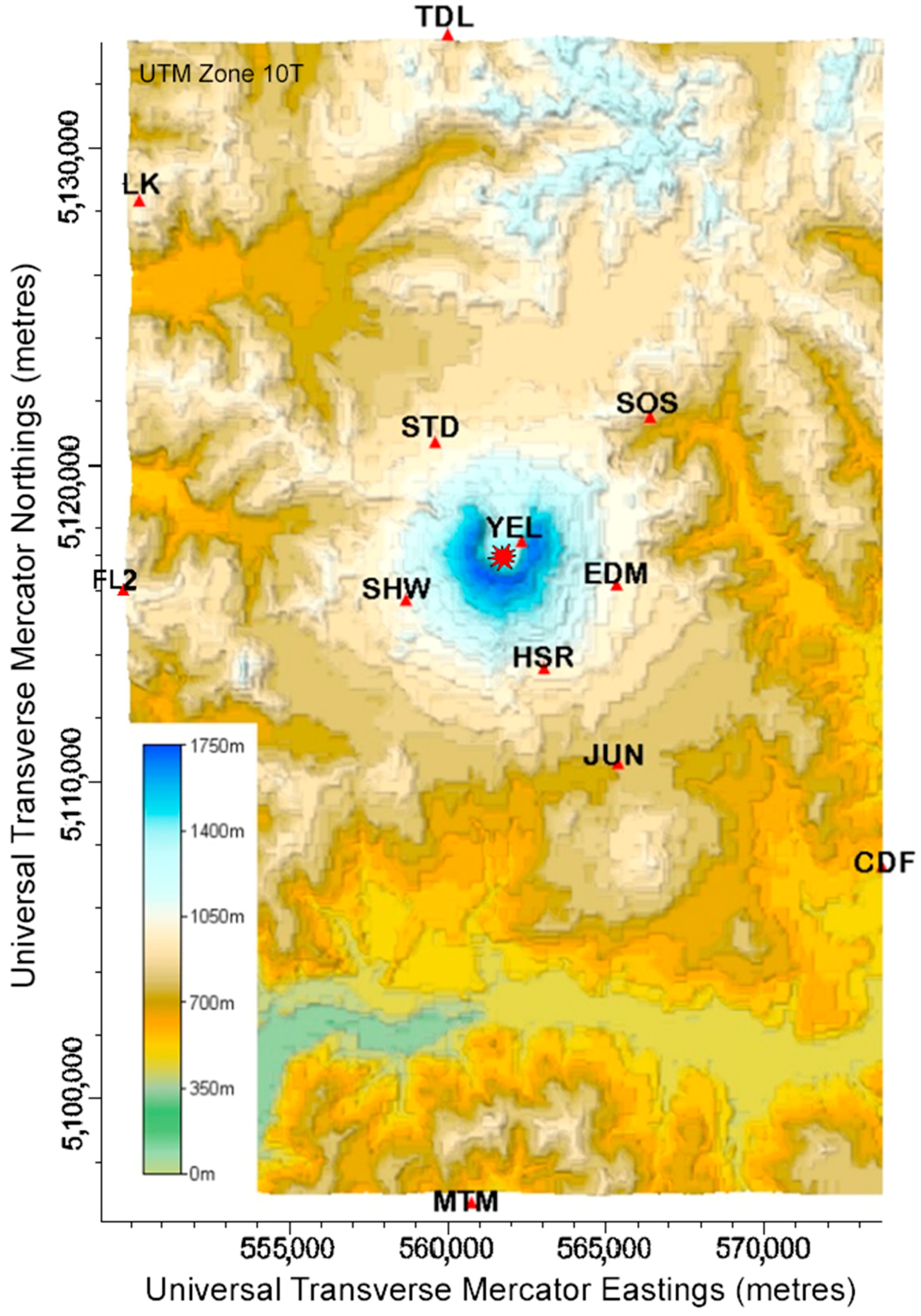
The timing and energy of this repeating source was remarkably consistent, and so it presents an opportunity to treat this dataset as an active source experiment. Utilising the Pacific Northwest Seismic Network, data recorded between 26 September 2004 and 29 December 2004 were selected at stations located as shown in Figure 4 (red triangles). Approximately 2400 vertical component traces were selected, based on the timings of seismic arrivals and signal to noise ratios. This was done to ensure that we were processing “drumbeat” arrivals and that sites with particularly noisy datasets (e.g., YEL on the summit crater) did not distort the final results.
3.2. Diffusion Model Theory
One of the principle methods currently used in modelling wave propagation through random media is radiative transfer theory (e.g., Sato and Fehler, 1998 [7]). This technique assumes a velocity structure described by a random medium, and characterised by its autocorrelation function and the mean value of the background velocity. The propagating seismic energy is divided into two alternative processes: the free propagation in an effectively homogenous background medium, and the scattering caused by point-like scatterers.
At the extreme limit of strong multiple scattering, Wegler (2003) demonstrated that the diffusion model (e.g., Dainty and Toksov (1981) [29]) can describe a homogeneous and isotropic random medium by taking an acoustic approximation of the coda in Equation (1).
where W(r,t) is the density of seismic energy and p is a dimensional constant. For body waves p = 3 and for surface waves p = 2. As surface waves have been observed to strongly affect the coda at low frequencies (<3 Hz) [30,31], the dominance of body waves is assumed. The diffusion coefficient is related to the physical medium by the transport mean free path and seismic velocity v by:
where the transport mean free path is given by Gusev and Abubakirov (1996) [27]:
In the case of non-isotropic scattering as assumed by this study, the angular dependent scattering coefficient is described by , where is the scattering angle and describes how energy loses memory of its initial direction of propagation. With the strong multiple scattering observed in random highly-heterogeneous media, it is the parameter that primarily controls coda generation [32]. The reciprocals of and are calculated to connect these coefficients to the physical medium. These are also known as the scattering mean free path and the transport mean free path respectively. By taking the reciprocal of we can connect the results to the physical medium in the form of the transport mean free path to fit the data to the diffusion model in the time domain, the method of Wegler and Lühr (2001) [8] is used. Multiplying Equation (1) by the geometrical factor and taking the logarithm results in:
This equation demonstrates that, for a fixed distance r as a function of time t, parameter W depends linearly on three base functions: 1, t, and 1/t. To calculate the three associated unknowns, , and , a linear least squares inversion is applied and using the following equations the physical parameters of E0, b and d are then given by:
To ensure consistent data processing, an automated routine was developed in MatLab (see supplementary material) to apply the diffusion approximation to the seismic arrivals. However, some differences do apply depending on the location of the recording station. At MSH, we assume two separate scattering regimes that are both dominated by body waves. Firstly, a strongly scattering region near to the volcano and secondly, outside this area, a much weaker scattering environment. Since we cannot know the true length of the raypath within the strongly scattering volcanic edifice, distances have been simplified into two groups. Those that are found at stations off the volcano (CDF, ELK, FL2, MTM and TDL are the station short names) and stations that are found on the volcanic edifice itself (EDM, HSR, JUN, SHW, STD, SOS and YEL are the station’s short names). For use in Equation (4), ray path lengths (r) are initially set to 10 km for the first group and 4 km for the second, respectively.
To calculate seismic energy density W, tmin is set as the P-arrival and tmax (see Figure 5) is defined when the amplitude approaches zero after the initial onset. The width of the energy windows used to measure W is defined as tmax minus tmin divided by 5. By using a small number of windows, we better depict the near-receiver geological overprint.
3.3. Data Processing
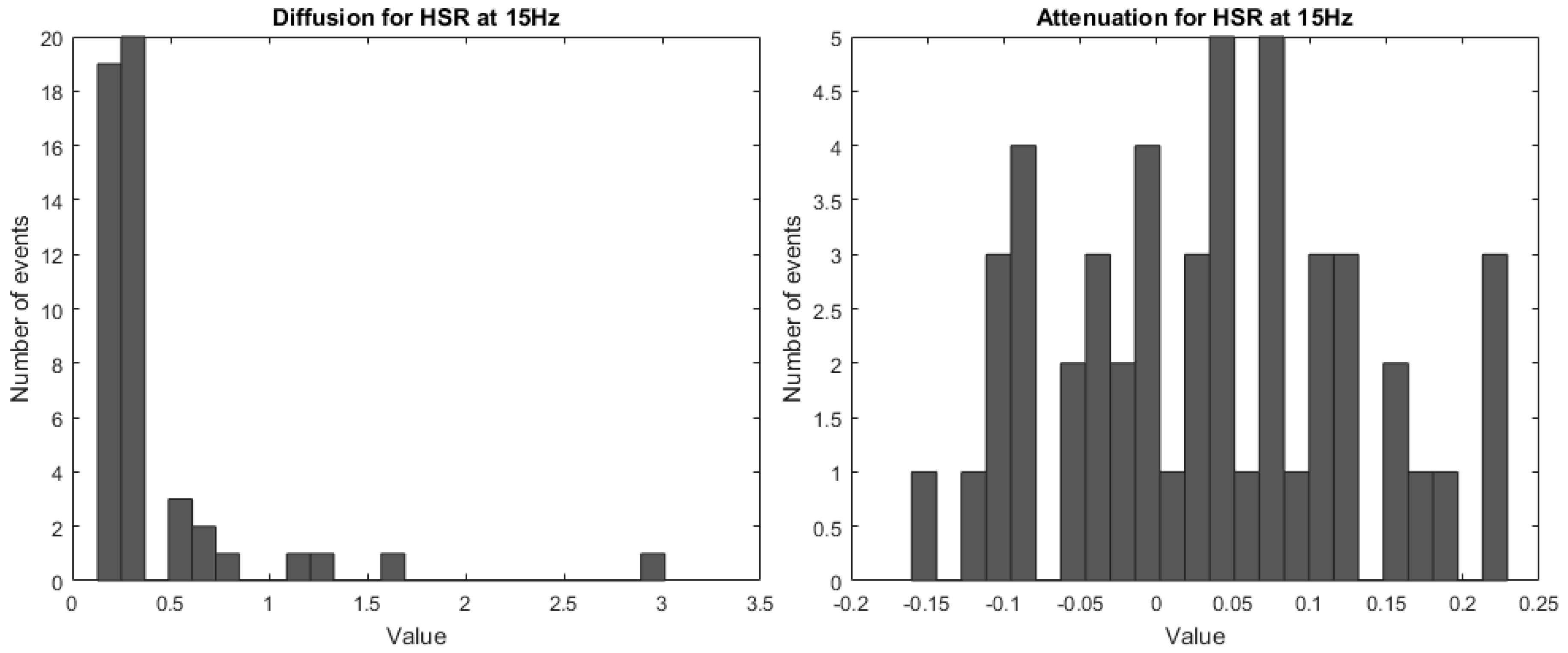
The first step to processing the inversion results is to apply an averaging procedure to calculate a mean value for each seismic recording station. Results from each station are separated and NaN or infinite values are removed. A histogram count is then applied, where the number of bins is defined as the number of traces for that station divided by two, minus one. This is performed to minimise the effects of a small number of arrivals at certain stations distorting the results with outliers. A mean is then calculated from those values which are within the limits of the most populous bin. By applying this procedure, results are weighted towards to the most common values. If two or more bins have the same number of values, the averaging limits are defined as the minimum and maximum values of the outer bins. An example of histograms plots is shown in Figure 6. Table 1 is the output of this procedure where on-volcano stations have been marked in italic.
The same data are plotted in Figure 7 with associated error bars. Where the error is defined as the standard deviation of the values used for averaging. For both groups of stations, the diffusion error is observed to increase with frequency but a far larger range in values is seen for off-volcano stations, which can be attributed to the breakdown of the diffusive approximation at far offsets. Another important difference is that values for on-volcano stations do not greatly vary as frequency increase. Whilst increasing the offset and change into the off-volcano regime, there is an obvious trend for values to increase with frequency. Values for the attenuation coefficient behave similarly for both scattering regimes in that there is a negative trend as frequency increases. However, the error range for on-volcano stations is typically larger.
To assess the level of confidence that can be ascribed to these results as well as the impact of the ray-path length, r, simplification, theoretical diffusion curves are compared with the observed seismic energy density measurements, which have been stacked for each station. Figure 8 shows an example of a good model fit at the two offsets. Depending on the frequency, the fit becomes poorer as errors in coefficient measurement and uncertainty in r estimation increase. Fit values at the central frequency of 9 Hz, which showed the best fit at all stations, in our analysis range are shown in Table 2.
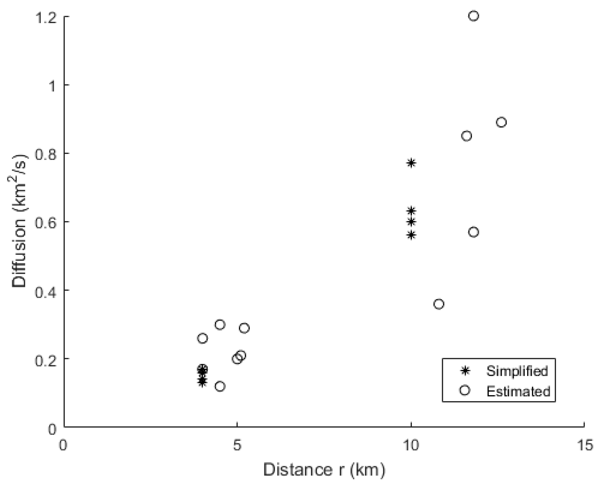
To quantify the level of fit between the theoretical data and the observed, a two-sample Kolmogorov–Smirnov test was performed to assess the likelihood that both datasets came from the same distribution. This test quantifies the distance between the empirical distribution function of the observed data and the cumulative distribution of the theoretical. The outputs is a value of probability that both datasets came from the same distribution. With testing, it was observed that source-receiver distance played a large role in determining the diffusion coefficient and so controlled the theoretical seismic energy density. A simple routine was devised with fixed coefficient parameters that iterated values for r until a sufficient level of probability was acquired. Values for estimated r began at 20 km and were reduced by 0.1 km for each iteration. If the estimated value dropped below half the simplified distance, i.e., 4 km or 10 km, the routine was stopped, the probability threshold was lowered and the process restarted. New values for r are then applied to the inversion procedure to generate new diffusion and attenuation coefficients. By doing this we improve the fit of measured data to the theoretical diffusion approximation and provide a better estimation of the true raypath lengths that would occur within this model. Table 3 displays the new fit values, including values for estimated r and the diffusion coefficient. Figure 9 is a plot comparing the distribution of values of diffusion for the simplified and estimated results. Whilst there is some change in values, at the limited resolution of this methodology and the uncertainty at far offsets, the distribution of data points is sufficient to say that the use of simplified values for r is adequate.
4. Results and Discussion
4.1. Diffusion
At the short lapse times from the P-wave arrival we consider, Calvet and Margerin (2013) [33] demonstrate that coda measurements are most sensitive to the effects of scattering, with temporal decay of the seismogram at later lapse times being mostly dependent on absorption effects. This is not necessarily valid at 3 Hz, where the LP sources show a resonant coherent component [15]. In strongly heterogeneous media and using volcano-tectonic events, Wegler (2003) [9], Gao and Zhang (2013) [34] and De Siena et al. (2014) [12] confirm that at short lapse times scattering may be affected by local topography and is frequency dependent, with lower frequencies being most sensitive to heterogeneity at the surface. De Siena et al. (2016) [13] go further, showing the potential of coda waves for imaging the 30-m-thick debris flows of the 1980 MSH eruption.
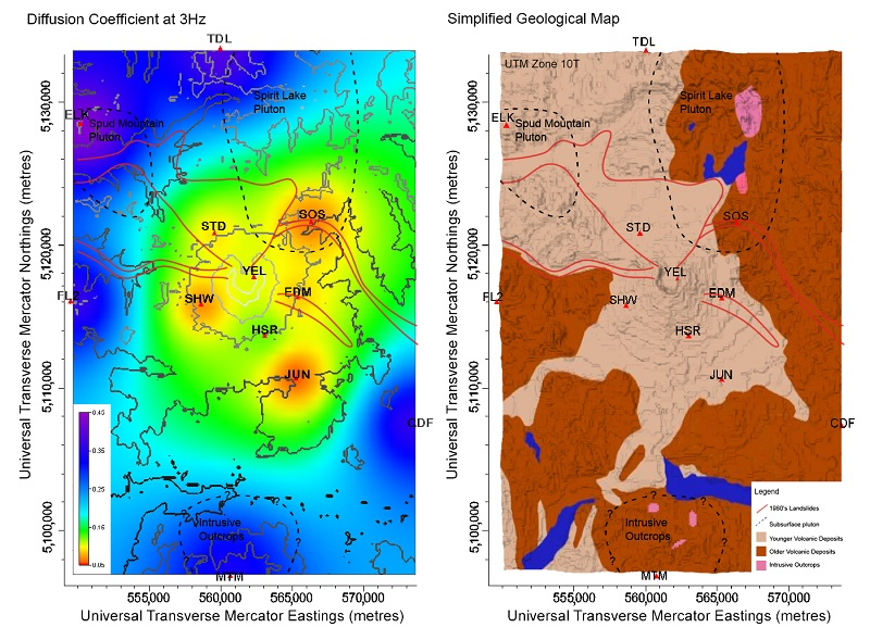
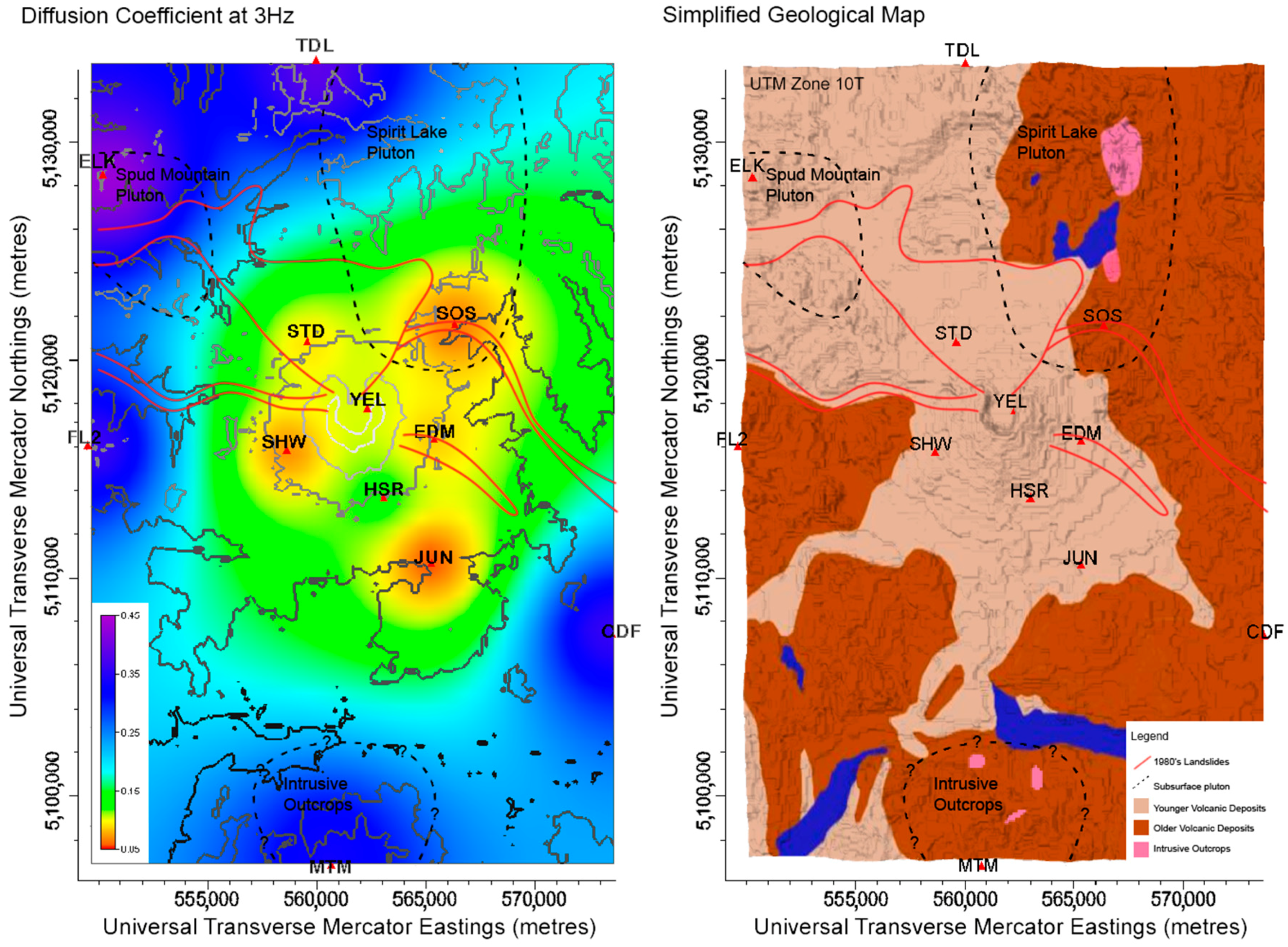
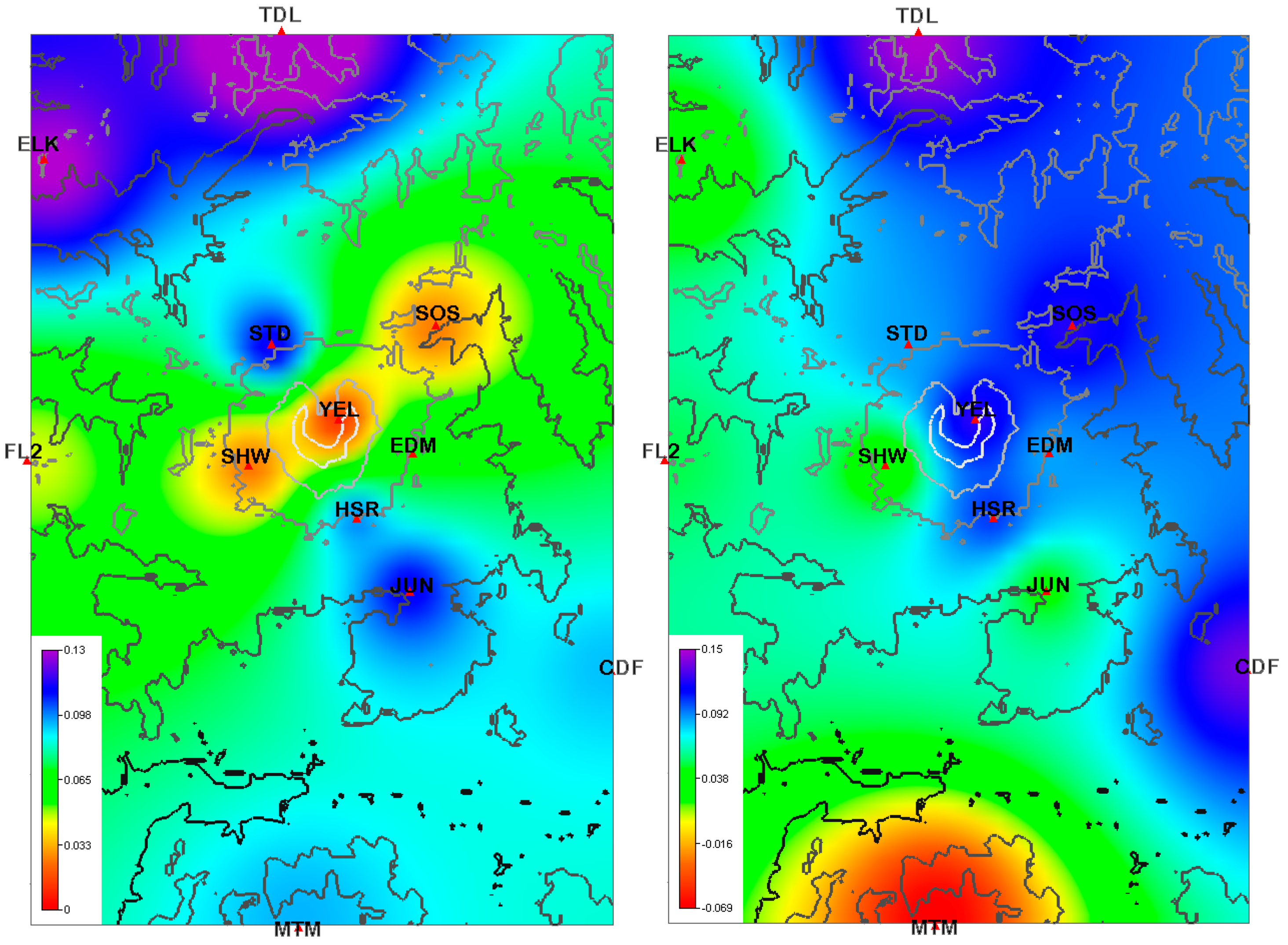
These observations provide the framework for Figure 10. Results for the diffusion coefficient at 3 Hz are plotted at each recording station and gridded using an inverse distance method in Voxler (see supplementary material for an example data plot). The maps show strong local minima/maxima but can be seen to correlate with known near-surface geological features. A low-diffusivity anomaly is observed around the volcanic cone; as the offset from the volcanic centre increases, diffusivity is seen to increase rapidly. Since the diffusion coefficient is derived from the mean free path, diffusivity is the inverse of scattering. The strongest scattering is observed at stations positioned on Pleistocene–Recent deposits. Slightly smaller amounts of scattering are found at stations EDM and STD, which are located on landslide material from the 1980’s eruption. Station HSR, and to a degree YEL, is notable in that is understood to be close to glacial deposits but not close to recent landslide material [35]. In media where ice and water are trapped, diffusivity increases consistently resulting in the lower amounts of scattering observed [36]. Outside of the strongly scattering regime, in the outskirts of MSH, the diffusion coefficient shows values that would be expected for single-to-weakly scattering media. Stations FL2 and CDF have average values, with the highest values being located at sites close to known plutonic intrusions. The variance that is seen within the two regimes is strongly dependent on the source-receiver distance and the coherency of larger-scale structures close to the seismic receiver. By increasing the offset value r, the diffusion coefficient rapidly increases, and so the simplification introduced in the model may mean that differences can be attributed to the resonant source signature or an incorrect estimation of r.
On the other hand, diffusion coefficient results at 3 Hz suggest that such differences can also be attributed to large coherent reflecting surfaces dominating the principle scattering direction. This is the case close to plutonic structures, such as station ELK. Here, the strong acoustic impedance contrast between the intrusion and country rock reduces the apparent diffusivity, as the interaction with the interface overshadows the effects of smaller-scale geological structure [37]. The same result can be observed at stations positioned on landslide material, where instead of an increased amount of scattering that would be expected for such chaotic deposits, there is a relative decrease. In our interpretation, this is due to the creation of landslide blocks during the 1980s eruption [13], resulting in several large coherent slip planes for seismic energy to be scattered at.
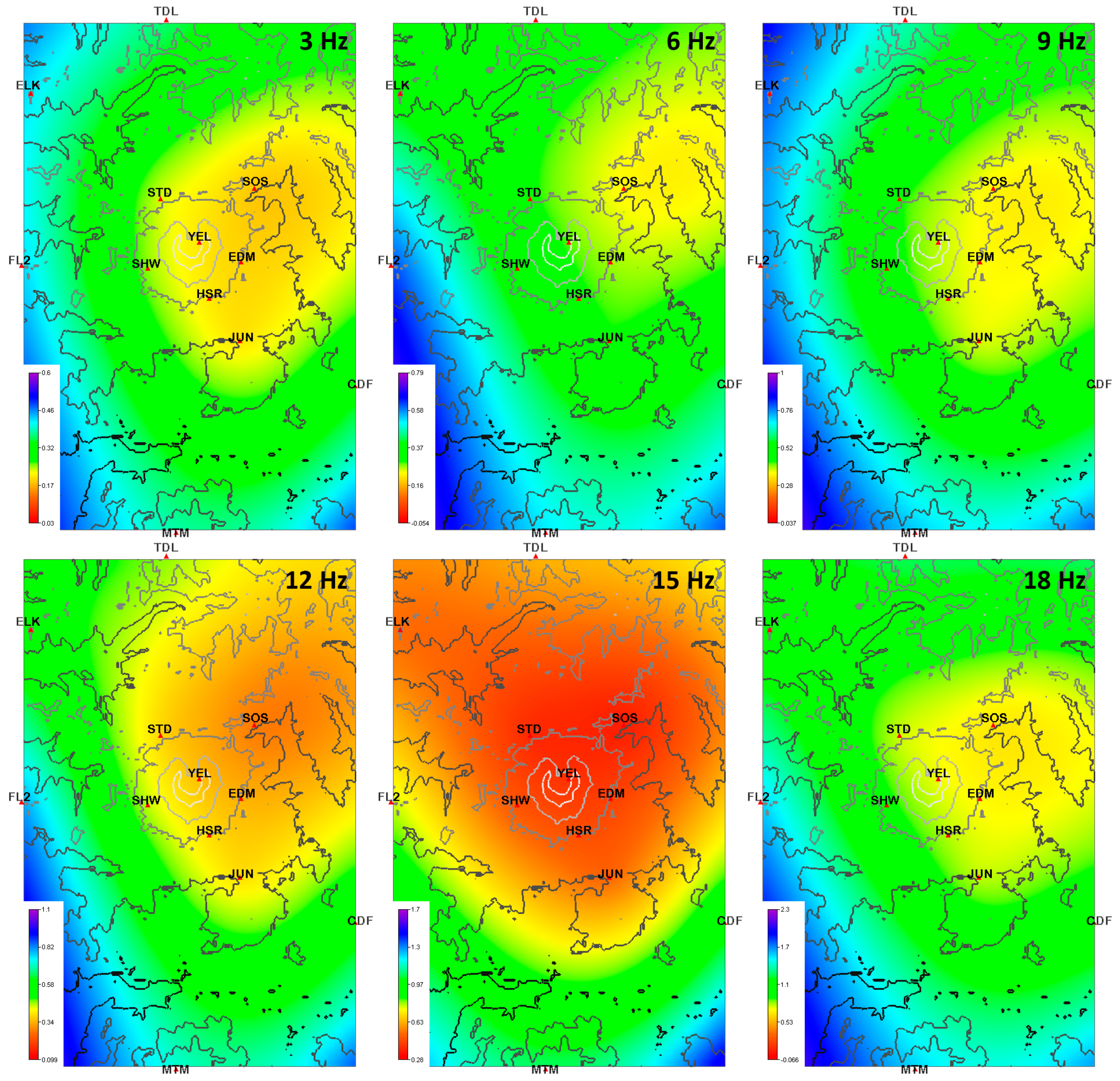
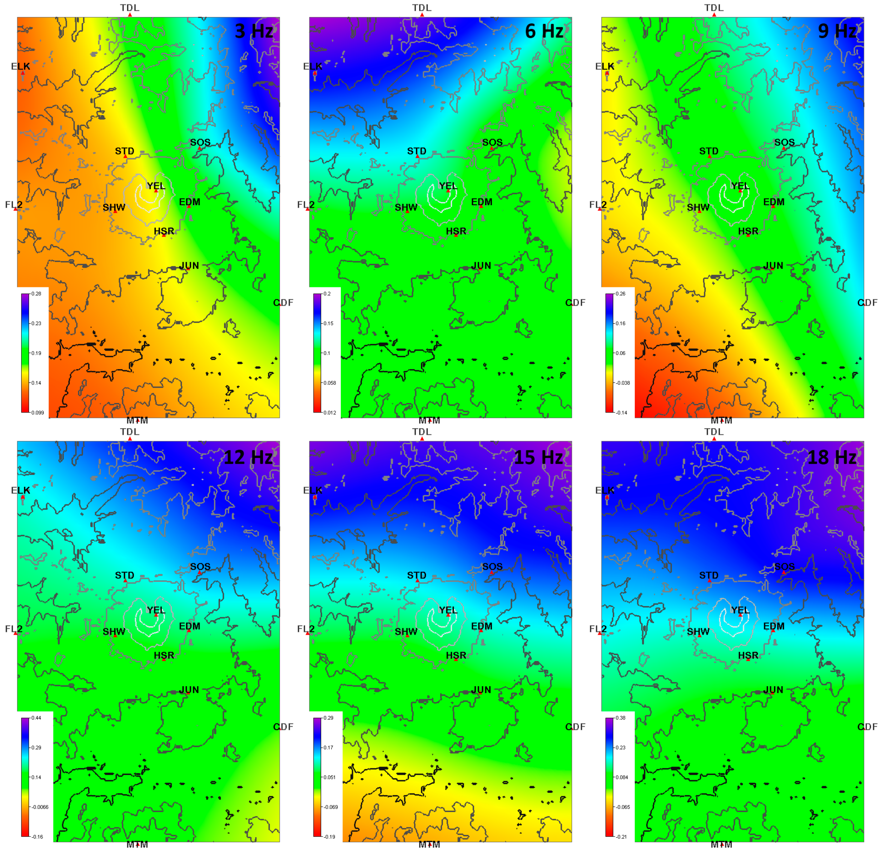
Plotting results using a local polynomial method in Figure 11 yields tomographic maps that better correlate with previously observed regional trends. At 3 Hz a scattering anomaly following a NE-SW trend is observed. It encompasses the volcanic edifice and stretches to the NE. Between 6 Hz and 9 Hz this feature is shifted down and to the east. From 12 Hz to 15 Hz the amount of scattering rapidly increases in amplitude and area, fully comprising the volcanic edifice and the north of the study area. AT 18 Hz the anomaly is reduced and is in a E-W orientation but is shifted to the right of the volcanic edifice as observed at the lower frequencies.
Further confirmation of the invalidity of the diffusion approximation at far-offsets is found when calculating the average transport mean free path, , for on and off volcano stations. Maintaining the assumption that there are two separate scattering regimes, velocity is defined as 2 km/s and 5 km/s respectively. Within the frequency range 3–18 Hz, a value of is obtained for on-volcano stations and for off volcano. is comparable with typical values of between 100 m and 1000 m found at other volcanic sites [8,9,38,39,40,41,42] where scattering effects have been observed to dominate over intrinsic attenuation. However, away from the strongly scattering regime close to a volcano, typical crustal values are in the range of and so for off-volcano stations is several orders of magnitude lower than it should be. Again, this can be attributed to the uncertainty in ray path length and unsuitability of the diffusion model at these far offsets.
The interpretation follows that of De Siena et al. (2016) [13], where the attenuation and scattering parameters observed at different frequencies are depth dependent, with increasing frequency sampling deeper structure. At shallow depths (<200 m) the low frequency coda is strongly affected by surface waves [30,31] and so at 3 Hz the scattering anomaly is associated with the scattering volcanic edifice but is also strongly affected (as are all measured frequencies) by the presence of high scattering anomalies to the NE and E of the volcano. From 6 Hz to 9 Hz features are associated with the SHZ reducing the amount of observed scattering, suggesting a strongly coherent boundary forming this feature at 2.9 km depth. The increased amount of scattering that is observed between 12 Hz and 15 Hz can be correlated with the interpretation of De Siena et al. (2014) [12] of a very strongly scattering magma chamber. In the study, the authors observe a rapid broadening of this chamber which then floors off after 4 km depth. At 18 Hz features switch to a E-W trend that is associated with deeper regional magmatic structure and feeding systems [21].
4.2. Attenuation
Unlike the diffusion coefficient, which is structurally and source controlled, the attenuation coefficient is more sensitive to media properties. Quantities like pore fluid and relative seismic velocity control attenuation by either directly attenuating a propagating ray or by increasing the length of time the seismic energy is within a medium [11]. However, in the diffusive approximation, the large uncertainties associated to average mean values (e.g., Figure 7) as well as the onset of “negative attenuation”, which is suggestive of resonant processes [35] both translate in high uncertainty in the properties of the sampled medium. Some correlations with known geological features can be seen at 9 Hz, in Figure 12. As observed by Waite and Moran (2009) [20], MSH sits atop a significant NW-SE anomaly, which is related to regional plate tectonics. Between depths of 10 km and 14 km, the boundary shows the contrast between the south-western high-velocity and low-attenuation Siletz Terrane and the north-eastern low-velocity, high attenuation Cascade Arc Crust [12,43].
Spatial correlations can also be seen at 6 Hz with the results from De Siena et al. (2016) [13]. In the study, the authors observe high coda attenuation values to the NW and SE of the volcanic edifice at 18 Hz, which correlate with regions of high attenuation as seen in Figure 10. The authors show a region where waveforms are characterised by higher S-wave peak delays, which stretches across the volcanic edifice in the NE-SW direction. High peak-delays are indicative of strong forward scattering and correlate with the lowest values of attenuation in our results; in our interpretation, seismic energy is quickly scattered away from these regions before being attenuated by local heterogeneities.
As before with the diffusion coefficient, gridding attenuation results with a local polynomial means that we lose the local scale sensitivity as assumed by the method, but better correlation can be observed with regional trends. In Figure 13, High attenuation areas correlate well with areas of low rise-times and Qc−1 at 6 Hz and 9 Hz, with high-rise times being associated with regions of very low attenuation as shown in De Siena et al. (2016) [13]. With increasing frequency, the rotation and shift of tectonic trend is observed to go from a strong NW-SE orientation to E-W with areas of high attenuation having a more westwards expression in the NE of the study area. 3 Hz is very notable in that unlike the diffusion coefficient, it does not correlate well with the surface geology but instead follows the regional trend of the SHZ separating the Siletz and Cascade Arc terranes. Again, this can be attributed to surface waves having a strong effect on the seismic coda at these low frequencies, resulting in a combination of shallow and deep structure information being present in the results.
5. Conclusions
We use the diffusive approximation of the dispersion of seismic energy within strongly scattering media and data from a highly repetitive, natural source to measure station-dependent diffusion and attenuation coefficients at Mount St. Helens volcano, USA. Both factors are then spatially mapped as a property of the near-receiver medium. The results show important correlation with the local geology and improve our interpretation of up to 5 km deep volcanic structures.
At 3 Hz, values for the diffusion coefficient correlate with known near-surface geological structures. A weakly diffusive (strongly scattering) volcanic centre is observed close to the source, possibly as an effect of source resonance. At further offsets, the diffusivity values rapidly increase, as the complexity of the near-surface geology decreases, large-scale coherent structures become more prevalent, and the wave field loses its resonant source characteristics. This dominance of coherent structure effects is evident close to the volcano, at receivers positioned on landslide material, where scattering is observed to be lower than for media of similar composition at other receivers.
At 6 Hz, areas of high attenuation to the NW and SE correlate with regions of high coda attenuation as observed by De Siena et al. (2016) [13], as well as a region of low attenuation and high-rise times directly beneath the volcanic edifice. High attenuation at 9 Hz is observed in regions of low seismic velocity to the NE of the volcanic edifice, following the gentle dip toward NE of the plumbing system [16]. High attenuation also corresponds to a zone of high-velocity and low scattering [13,16] to the SW of the volcanic edifice, where evidence of prehistorical volcanic activity are visible.
The mapping methodology we propose does not require a velocity model and is robust enough for a simplified estimation of receiver-dependent diffusivity and attenuation within strongly scattering media, while, due to the sudden break of the diffusion approximation, uncertainties become increasingly larger at far offsets, i.e., into single-to-weakly scattering regimes.
Supplementary Materials
The following are available online at www.mdpi.com/2076-3263/7/4/130/s1; MatLab R2016a (9.0.0.341360) codes for inversion results and theoretical plots, Voxler (4.2.584) file for data visualisation.
Acknowledgments
The SAGES VALIDATE forum provided travel money for the discussion of the methodology within De Siena and Benson.
Author Contributions
Luca De Siena conceived and supervised the initial MSc project and provided expertise on the field methodology; Thomas King performed the experiments and analysed the data; Phil Benson and Sergio Vinciguerra provided substantial feedback in terms of focus and the current state of volcanology and rock physics; Thomas King wrote the paper. All authors edited the manuscript, improving text and interpretations.
Conflicts of Interest
The authors declare no conflict of interest.
References
- Ferreira, A.M.G.; Woodhouse, J.H. Source, Path and receiver effects on seismic surface waves. Geophys. J. Int. 2007, 168, 109–132. [Google Scholar] [CrossRef]
- Shearer, P.M.; Orcutt, J.A. Surface and near-surface effects on seismic waves—Theory and borehole seismometer results. Bull. Seismol. Soc. Am. 1987, 77, 1168–1196. [Google Scholar]
- Neuberg, J.; O’Gorman, C. A Model of the Seismic Wavefield in Gas-Charged Magma: Application to Soufriere Hills Volcano, Montserrat; Memoirs 21.1; Geological Society of London: London, UK, 2002; pp. 603–609. [Google Scholar]
- Bean, C.; Lokmer, I.; O’Brien, G. Influence of near-surface volcanic structure on long-period seismic signals and on moment tensor inversions: Simulated examples from Mount Etna. J. Geophys. Res. Solid Earth 2008, 113. [Google Scholar] [CrossRef]
- Aki, K. Analysis of the seismic coda of local earthquakes as scattered waves. J. Geophys. Res. 1969, 74, 615–631. [Google Scholar] [CrossRef]
- Aki, K. Attenuation of shear-waves in the lithosphere for frequencies from 0.05 to 25 Hz. Phys. Earth Planet. Inter. 1980, 21, 50–60. [Google Scholar] [CrossRef]
- Sato, H.; Fehler, M.C. Seismic Wave Propagation and Scattering in the Heterogeneous Earth; Springer: Berlin, Germany, 1998. [Google Scholar]
- Wegler, U.; Lϋhr, B.-G. Scattering behaviour at Merapi volcano (Java) revealed from an active seismic experiment. Geophys. J. Int. 2001, 145, 579–592. [Google Scholar] [CrossRef]
- Wegler, U. Analysis of multiple scattering at Vesuvius volcano, Italy, using data of the TomoVes active seismic experiment. J. Volcanol. Geotherm. Res. 2003, 128, 45–63. [Google Scholar] [CrossRef]
- Sato, H.; Fehler, M.C.; Maeda, T. Seismic Wave Propagation and Scattering in the Heterogeneous Earth, 2nd ed.; Springer: New York, NY, USA, 2012; 494p. [Google Scholar]
- Mavko, G.; Mukerji, T.; Dvorkin, J. The Rock Physics Handbook: Tools for Seismic Analysis of Porous Media; Cambridge University Press: Cambridge, UK, 2009. [Google Scholar]
- De Siena, L.; Thomas, C.; Waite, G.P.; Moran, S.C.; Klemme, S. Attenuation and scattering tomography of the deep plumbing system of Mount St. Helens. J. Geophys. Res. 2014, 119, 8223–8238. [Google Scholar] [CrossRef]
- De Siena, L.; Calvet, M.; Watson, K.J.; Jonkers, A.R.T.; Thomas, C. Seismic scattering and absorption mapping of debris flows, feeding paths, and tectonic units at Mount St. Helens. Earth Planet. Sci. Lett. 2016, 442, 21–31. [Google Scholar] [CrossRef]
- Cheney, E.S. What is the age and extent of the Cascade Magmatic Arc? Wash. Geol. 1997, 25, 28–32. [Google Scholar]
- Waite, G.P.; Chouet, B.A.; Dawson, P.B. Eruption Dynamics at Mount St. Helens Imaged from Broadband Seismic Waveforms: Interaction of the Shallow Magmatic and Hydrothermal Systems. J. Geophys. Res. 2008. [Google Scholar] [CrossRef]
- Kiser, E.; Palomeras, I.; Levander, A.; Zelt, C.; Harder, S.; Schmandt, B.; Hansen, S.; Creager, K.; Ulberg, C. Magma reservoirs from the upper crust to the Moho inferred from high-resolution VP and Vs models beneath Mount St. Helens, Washington State, USA. Geology 2016, 44, 411–414. [Google Scholar] [CrossRef]
- Moran, S.C.; Lees, J.; Malone, S. P wave crustal velocity structure in the greater Mount Rainier area from local earthquake tomography. J. Geophys. Res. 1999, 104, 10775–10786. [Google Scholar] [CrossRef]
- Lees, J.M. The magma system of Mount St. Helens; non-linear high-resolution P wave tomography. J. Volcanol. Geotherm. Res. 1992, 53, 103–116. [Google Scholar] [CrossRef]
- Nolet, G. Seismic wave propagation and seismic tomography. In Seismic Tomography; Springer: Dordrecht, The Netherlands, 1987; pp. 1–23. [Google Scholar]
- Waite, G.P.; Moran, S.C. VP Structure of Mount St. Helens, Washington, USA, Imaged with Local Earthquake Tomography. J. Volcanol. Geotherm. Res. 2009, 182, 113–122. [Google Scholar] [CrossRef]
- Hill, G.J.; Caldwell, T.G.; Heise, W.; Chertkoff, D.G.; Bibby, H.M.; Burgess, M.K.; Cas, R.A. Distribution of melt beneath Mount St Helens and Mount Adams inferred from magnetotelluric data. Nat. Geosci. 2009, 2, 785–789. [Google Scholar] [CrossRef]
- Hansen, S.M.; Schmandt, B.; Levander, A.; Kiser, E.; Vidale, J.E.; Abers, G.A.; Creager, K.C. Seismic evidence for a cold serpentinized mantle wedge beneath Mount St Helens. Nat. Commun. 2016, 7, 13242. [Google Scholar] [CrossRef] [PubMed]
- Evarts, R.C.; Ashley, R.P.; Smith, J.G. Geology of the Mount St. Helens area: Record of discontinuous volcanic and plutonic activity in the Cascade Arc of southern Washington. J. Geophys. Res. 1987, 92, 10155–10169. [Google Scholar] [CrossRef]
- Poppeliers, C. The Effects of the Near-Surface Geology on P–S Strain Energy Partitioning of Diffusive Seismic Coda: Preliminary Observations and Results. Bull. Seismol. Soc. Am. 2015. [Google Scholar] [CrossRef]
- Huntting, M.T.; Bennett, W.A.G.; Livingston, V.E., Jr.; Moen, W.S. Geologic Map of Washington: Washington Division of Mines and Geology, Scale 1:500,000; Department of Natural Resources, Division of Geology and Earth Resources: Olympia, WA, USA, 1961. [Google Scholar]
- Vinciguerra, S.; Elsworth, D.; Malone, S. The 1980 pressure response and flank failure of Mount St. Helens (USA) inferred from seismic scaling exponents. J. Volcanol. Geotherm. Res. 2005, 144, 155–168. [Google Scholar] [CrossRef]
- Kendrick, J.E.; Lavallée, Y.; Hirose, T.; Di Toro, G.; Hornby, A.J.; De Angelis, S.; Dingwell, D.B. Volcanic drumbeat seismicity caused by stick-slip motion and magmatic frictional melting. Nat. Geosci. 2014, 7, 438–442. [Google Scholar] [CrossRef]
- Major, J.J.; Scott, W.E.; Driedger, C.; Dzurisin, D. Mount St. Helens Erupts Again; Activity from September 2004 through March 2005; U.S. Geological Survey: Reston, VA, USA, 2005; 4p.
- Dainty, A.M.; Toksōz, M.N. Seismic codas on the earth and the moon: A comparison. Phys. Earth Planet. Inter. 1981, 26, 250–260. [Google Scholar] [CrossRef]
- Galluzzo, D.; La Rocca, M.; Margerin, L.; Del Pezzo, E.; Scarpa, R. Attenuation and velocity structure from diffuse coda waves: Constraints from underground array data. Phys. Earth Planet. Inter. 2015, 240, 34–42. [Google Scholar] [CrossRef]
- Jing, Y.; Zeng, Y.; Lin, G. High-frequency seismogram envelope inversion using a multiple nonisotropic scattering model: Application to aftershocks of the 2008 wells earthquake. Bull. Seismol. Soc. Am. 2014, 104, 823–839. [Google Scholar] [CrossRef]
- Gusev, A.A.; Abubakirov, I.R. Simulated envelopes of non-isotropically scattered body waves as compared to observed ones: Another manifestation of fractal heterogeneity. Geophys. J. Int. 1996, 127, 49–60. [Google Scholar] [CrossRef]
- Calvet, M.; Margerin, L. Lapse-time dependence of coda Q: Anisotropic multiple-scattering models and application to the Pyrenees. Bull. Seismol. Soc. Am. 2013, 103, 1993–2010. [Google Scholar] [CrossRef]
- Gao, Y.; Zhang, N. Scattering cylindrical SH waves induced by a symmetrical V-shaped canyon: Near-source topographic effects. Geophys. J. Int. 2013, 193, 874–885. [Google Scholar] [CrossRef]
- Walder, J.S.; Schilling, S.P.; Sherrod, D.R.; Vallance, J.W. Evolution of Crater Glacier, Mount St. Helens, Washington, September 2006—November 2009; Open-File Report; U.S. Geological Survey: Reston, VA, USA, 2010; p. 34.
- Chaput, J.; Campillo, M.; Aster, R.C.; Roux, P.; Kyle, P.R.; Knox, H.; Czoski, P. Multiple scattering from icequakes at Erebus volcano, Antarctica: Implications for imaging at glaciated volcanoes. J. Geophys. Res. Solid Earth 2015, 120, 1129–1141. [Google Scholar] [CrossRef]
- De Siena, L.; Del Pezzo, E.; Thomas, C.; Curtis, A.; Margerin, L. Seismic energy envelopes in volcanic media: In need of boundary conditions. Geophys. J. Int. 2013, 195, 1102–1119. [Google Scholar] [CrossRef]
- Prudencio, J.; Ibáñez, J.; García-Yeguas, A.; Del Pezzo, E. Spatial distribution of intrinsic and scattering seismic attenuation in active volcanic islands, II: Deception island images. Geophys. J. Int. 2013, 195, 1957–1969. [Google Scholar] [CrossRef]
- Prudencio, J.; De Siena, L.; Ibáñez, J.; Del Pezzo, E.; García-Yeguas, A.; Díaz-Moreno, A. The 3D attenuation structure of Deception Island (Antarctica). Surv. Geophys. 2015, 36, 371–390. [Google Scholar] [CrossRef]
- Prudencio, J.; Del Pezzo, E.; Ibáñez, J.; Giampiccolo, E.; Patané, D. Two-dimensional seismic attenuation images of Stromboli Island using active data. Geophys. Res. Lett. 2015, 42. [Google Scholar] [CrossRef]
- Prudencio, J.; Aoki, Y.; Takeo, M.; Ibáñez, J.M.; Del Pezzo, E.; Song, W. Separation of scattering and intrinsic attenuation at Asama volcano (Japan): Evidence of high volcanic structural contrasts. J. Volcanol. Geotherm. Res. 2017, 333, 96–103. [Google Scholar] [CrossRef]
- Prudencio, J.; Taira, T.; Aoki, Y.; Aoyama, H.; Onizawa, S. Intrinsic and scattering attenuation images of Usu volcano, Japan. Bull. Volcanol. 2017, 79. [Google Scholar] [CrossRef]
- Parsons, T.; Blakely, R.J.; Brocher, T.M.; Christensen, N.I.; Fisher, M.A.; Flueh, E.; Kilbride, F.; Luetgert, J.H.; Miller, K.; ten Brink, U.S.; et al. Crustal structure of the Cascadia fore arc of Washington. In Earthquake Hazards of the Pacific Northwest Costal and Marine Regions; USGS Professional Paper; Kayen, R., Ed.; United States Geological Survey: Reston, VA, USA, 2005; Volume 1661D. [Google Scholar]
Figure 1.
Representative scattering behaviour of seismic energy due to differences in medium structure. (a) Loosely consolidated media exhibit strongly multiple-to-diffusive scattering ray behavior; (b) Highly consolidated/crystalline media typically show weakly-to-single scattering characteristics.
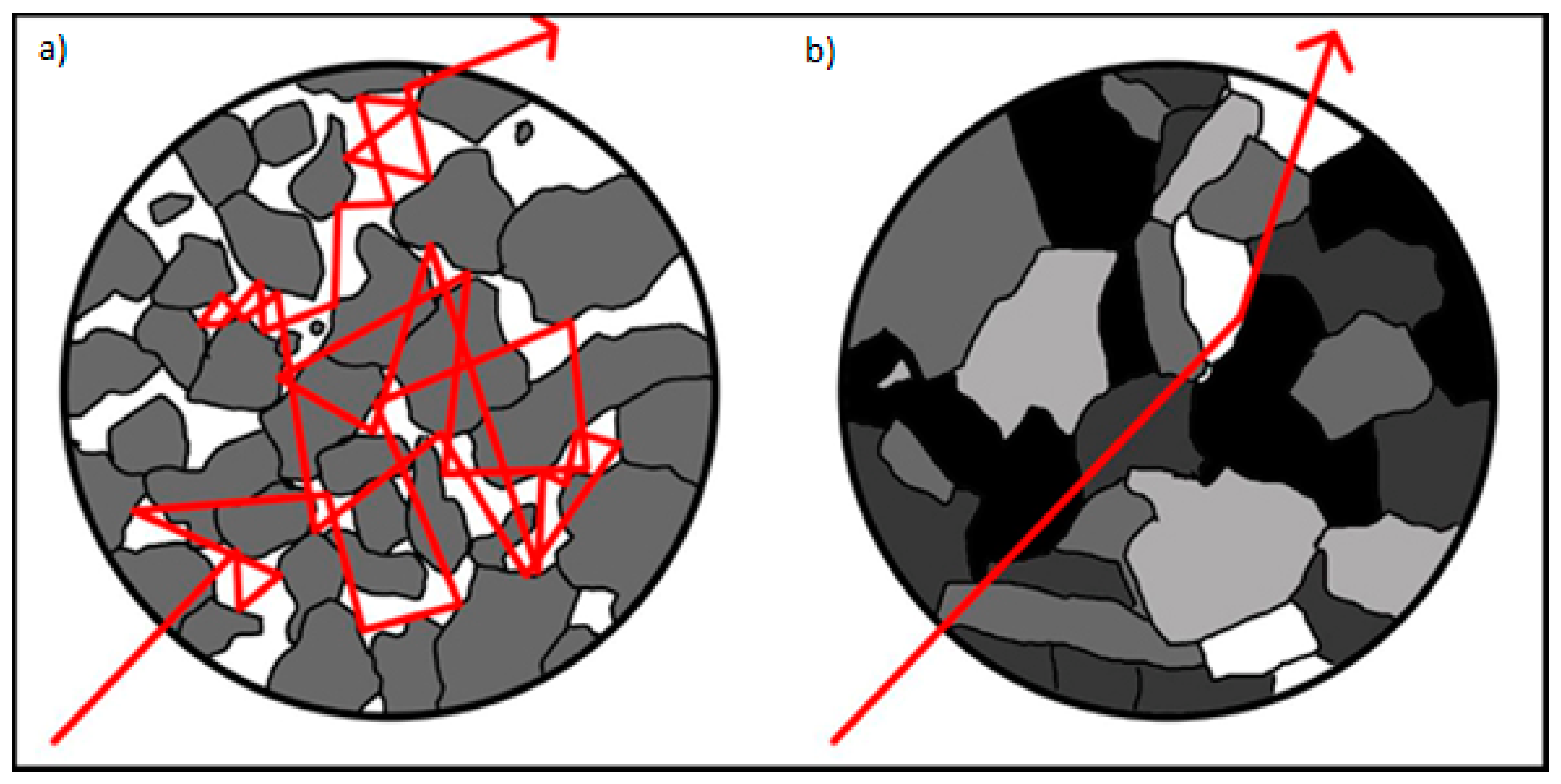
Figure 2.
Summary Geological Map of Mount St. Helens Volcano, USA, adapted from United States Geological Survey (USGS) [25]. Light brown shows Pleistocene–Recent age volcanic deposits and the darker brown, Oligocene–Miocene deposits. Pink areas and the dashed lines shows outcroppings of shallow subsurface plutons, whilst the red line maps out the extent of the 1980’s debris flows.
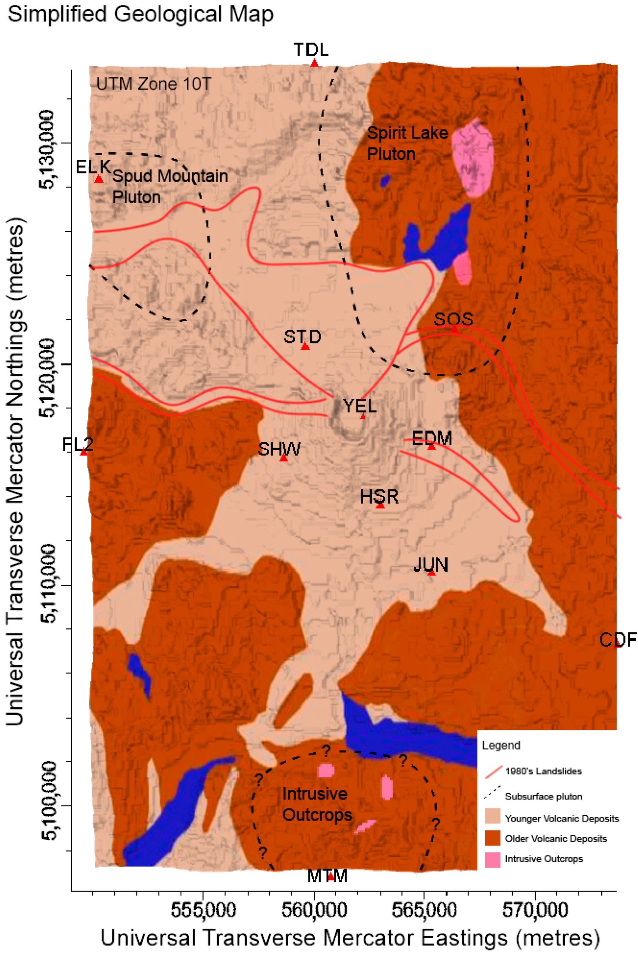
Figure 3.
Mount St. Helens Volcano crater schematic. A shallow hydrothermal fracture repeatedly opened and closed resulting in “drumbeat” seismicity at regular intervals. Modified from Major, J.J. et al. (2005) [28] and Waite et al. (2008) [15].

Figure 4.
Topographical map of Mount St. Helens volcano. Receiver stations used in the study are marked by red triangles. The LP drumbeat source is identified as a red star approximately 200 m beneath the growing dome.
Figure 4.
Topographical map of Mount St. Helens volcano. Receiver stations used in the study are marked by red triangles. The LP drumbeat source is identified as a red star approximately 200 m beneath the growing dome.

Figure 5.
Z-component of an example seismic arrival at stations STD and CDF filtered at 3 Hz, 6 Hz, 12 Hz and 18 Hz. Calculated envelopes, from which energy density is measured, are plotted below with the analysis windows between tmin and tmax indicated as vertical bars. Note the reduction in tmax as frequency increases.
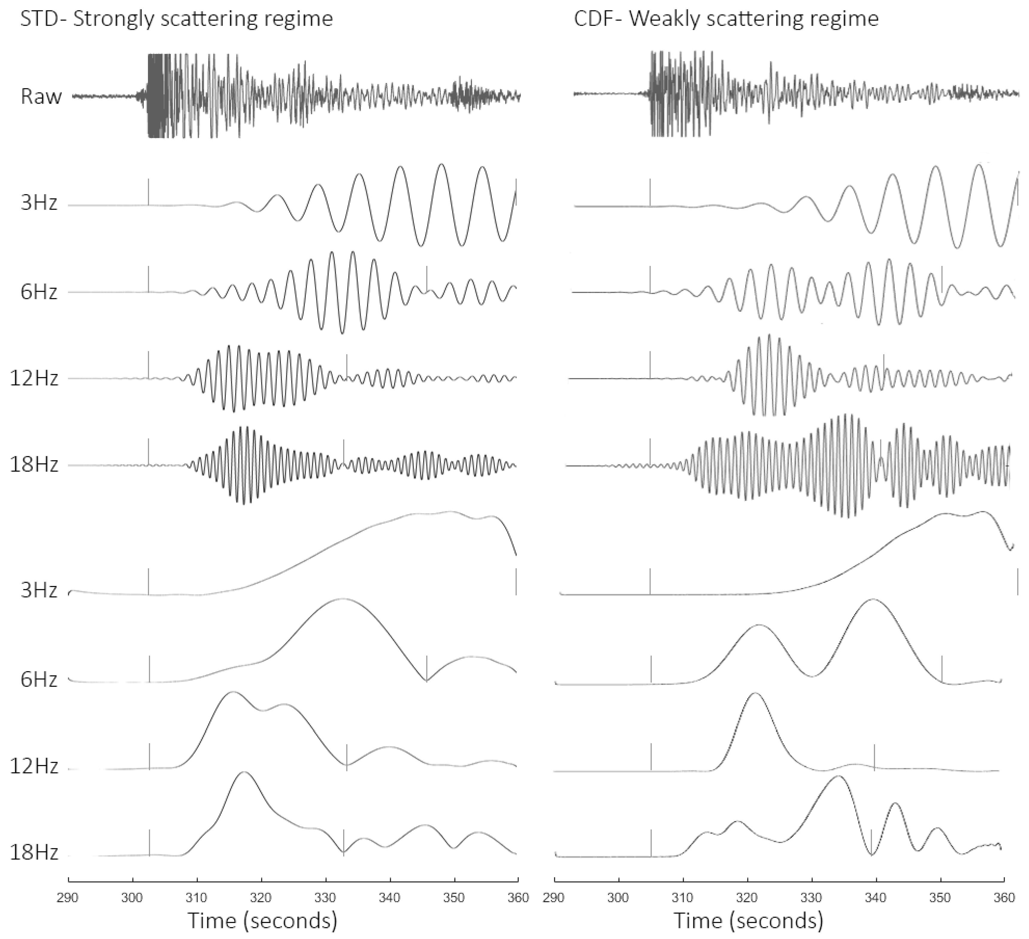
Figure 6.
Example histogram plots for station HSR at 15 Hz. Coefficient averages were taken from the most populous bins to minimise the effects of poor data distribution and outliers distorting results. When two or more bins have the same number of counts an average is calculated between the minimum and maximum values of those bins.

Figure 7.
Coefficient values plotted as a function of increasing frequency. Minimum and maximum of error bars are defined as the limits of the most populous histogram bin.
Figure 7.
Coefficient values plotted as a function of increasing frequency. Minimum and maximum of error bars are defined as the limits of the most populous histogram bin.
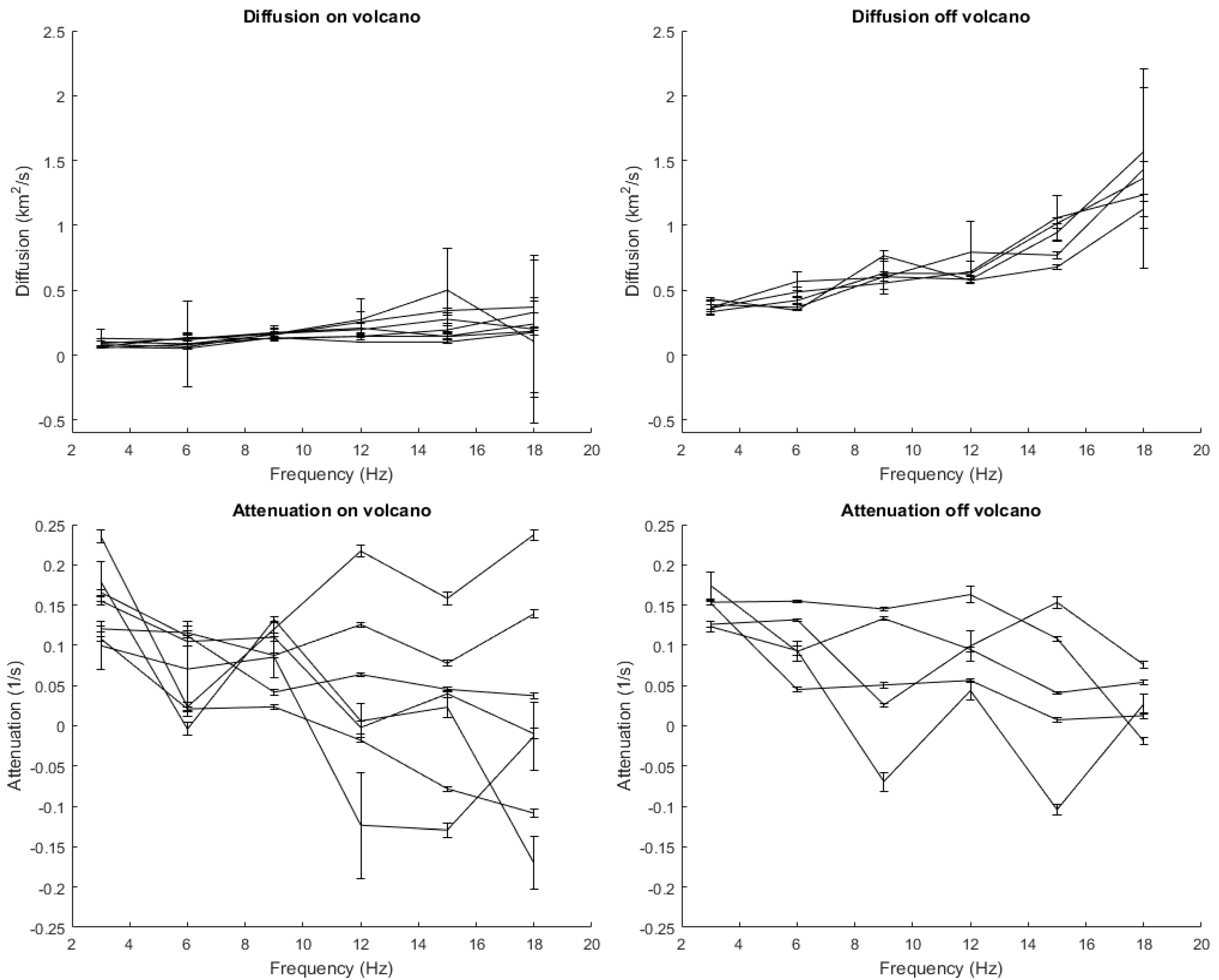
Figure 8.
Theoretical (dashed) vs. observed (solid) measurements for the logarithm of the averaged seismic energy density as corrected for geometrical spreading of body waves. By varying frequency the data fit can change quite drastically.
Figure 8.
Theoretical (dashed) vs. observed (solid) measurements for the logarithm of the averaged seismic energy density as corrected for geometrical spreading of body waves. By varying frequency the data fit can change quite drastically.
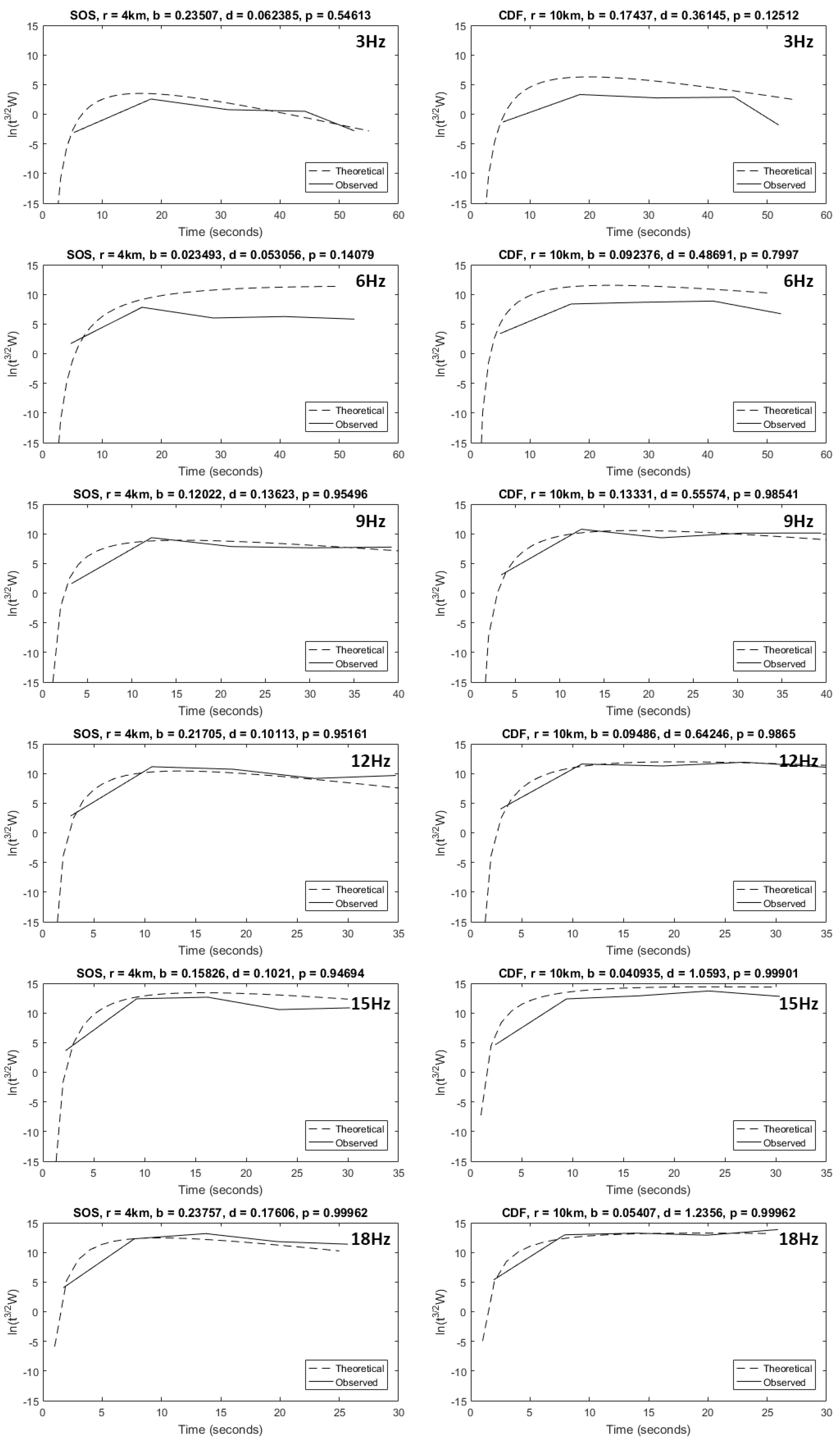
Figure 9.
Plot of diffusion coefficient values against source-receiver offset.

Figure 10.
Near-surface comparison of the diffusion coefficient (km2/s) at 3 Hz plotted using an inverse distance gridding method. The highest values for the diffusion coefficient are found closest to known intrusive deposits. The lowest values are found close to the volcanic edifice. Stations FL2 and CDF are found on older material and show average values. The map on the right is obtained interpolating the values obtained at different stations.

Figure 11.
Diffusion (km2/s) mapping gridded with a local polynomial method. 3 Hz is associated with a combination of near-receiver coda wave and deeper sampling from the surface wave. Increasing depth is associated with increasing frequency, and so the strongly scattering anomaly observed between 12 Hz and 15 Hz is attributed to a rapidly broadening magma chamber beneath and slightly to the NE of the volcanic edifice.

Figure 12.
Attenuation coefficient (1/s) spatially mapped using an inverse distance gridding method at 6 Hz (Left) and 9 Hz (Right).
Figure 12.
Attenuation coefficient (1/s) spatially mapped using an inverse distance gridding method at 6 Hz (Left) and 9 Hz (Right).

Figure 13.
Attenuation (1/s) mapping using a local polynomial method. As with Figure 12, results correlate with peak delay times but show a strong dependence on large scale regional trends.
Figure 13.
Attenuation (1/s) mapping using a local polynomial method. As with Figure 12, results correlate with peak delay times but show a strong dependence on large scale regional trends.


Table 1.
Mean inversion results for the diffusion and attenuation coefficient values for each recording station with associated error. Values in brackets next stations are the total number of events used in the histogram count after NaN and infinite values have been removed. Values in brackets next to coefficient values are the total number of events used to calculate average values.
| Diffusion | 3 Hz | 6 Hz | 9 Hz | 12 Hz | 15 Hz | 18 Hz |
| On Volcano | ||||||
| EDM (7) | 0.081 ± 0.027 (5) | 0.066 ± 0.017 (3) | 0.164 ± 0.041 (5) | 0.274 ± 0.159 (5) | 0.501 ± 0.319 (4) | 0.105 ± 0.626 (5) |
| HSR (49) | 0.13 ± 0.074 (44) | 0.12 ± 0.039 (43) | 0.166 ± 0.02 (19) | 0.197 ± 0.045 (35) | 0.277 ± 0.034 (25) | 0.201 ± 0.528 (43) |
| JUN (79) | 0.056 ± 0.001 (13) | 0.083 ± 0.004 (14) | 0.132 ± 0.007 (17) | 0.146 ± 0.011 (23) | 0.146 ± 0.022 (42) | 0.24 ± 0.526 (78) |
| SHW (77) | 0.066 ± 0.001 (13) | 0.137 ± 0.025 (39) | 0.126 ± 0.004 (15) | 0.145 ± 0.007 (14) | 0.195 ± 0.035 (33) | 0.331 ± 0.115 (49) |
| SOS (56) | 0.062 ± 0.004 (14) | 0.053 ± 0.007 (10) | 0.136 ± 0.009 (19) | 0.101 ± 0.003 (12) | 0.102 ± 0.014 (23) | 0.176 ± 0.019 (25) |
| STD (75) | 0.091 ± 0.018 (56) | 0.126 ± 0.048 (59) | 0.174 ± 0.054 (66) | 0.209 ± 0.049 (39) | 0.144 ± 0.019 (32) | 0.184 ± 0.027 (31) |
| YEL (9) | 0.103 ± 0.028 (8) | 0.088 ± 0.332 (8) | 0.157 ± 0.045 (5) | 0.255 ± 0.08 (8) | 0.344 ± 0.017 (5) | 0.371 ± 0.044 (4) |
| Off Volcano | ||||||
| CDF (98) | 0.361 ± 0.025 (28) | 0.487 ± 0.043 (33) | 0.556 ± 0.045 (32) | 0.642 ± 0.084 (45) | 1.059 ± 0.171 (66) | 1.236 ± 0.26 (78) |
| ELK (74) | 0.433 ± 0.015 (15) | 0.345 ± 0.005 (10) | 0.767 ± 0.041 (20) | 0.576 ± 0.013 (13) | 0.679 ± 0.018 (14) | 1.126 ± 0.057 (18) |
| FL2 (87) | 0.367 ± 0.058 (37) | 0.568 ± 0.074 (35) | 0.599 ± 0.029 (22) | 0.793 ± 0.237 (86) | 0.77 ± 0.03 (16) | 1.434 ± 0.768 (85) |
| MTM (26) | 0.335 ± 0.018 (7) | 0.422 ± 0.028 (10) | 0.632 ± 0.014 (7) | 0.628 ± 0.01 (7) | 1.015 ± 0.039 (6) | 1.364 ± 0.127 (15) |
| TDL (81) | 0.389 ± 0.054 (50) | 0.369 ± 0.024 (28) | 0.605 ± 0.136 (80) | 0.584 ± 0.023 (22) | 0.945 ± 0.066 (30) | 1.568 ± 0.497 (71) |
| Attenuation | 3 Hz | 6 Hz | 9 Hz | 12 Hz | 15 Hz | 18 Hz |
| On Volcano | ||||||
| EDM (7) | 0.1 ± 0.03 (3) | 0.07 ± 0.059 (3) | 0.085 ± 0.026 (4) | −0.124 ± 0.066 (3) | −0.129 ± 0.009 (3) | −0.013 ± 0.042 (4) |
| HSR (49) | 0.155 ± 0.005 (6) | 0.105 ± 0.005 (6) | 0.11 ± 0.005 (7) | −0.002 ± 0.007 (11) | 0.04 ± 0.004 (6) | −0.01 ± 0.007 (6) |
| JUN (79) | 0.166 ± 0.003 (12) | 0.112 ± 0.013 (19) | 0.042 ± 0.003 (8) | 0.064 ± 0.003 (9) | 0.045 ± 0.003 (8) | 0.037 ± 0.004 (9) |
| SHW (77) | 0.108 ± 0.003 (8) | 0.021 ± 0.003 (9) | 0.024 ± 0.003 (6) | −0.018 ± 0.003 (6) | −0.078 ± 0.003 (7) | −0.109 ± 0.005 (8) |
| SOS (56) | 0.235 ± 0.008 (11) | 0.023 ± 0.005 (6) | 0.12 ± 0.009 (11) | 0.217 ± 0.007 (6) | 0.158 ± 0.007 (9) | 0.238 ± 0.007 (7) |
| STD (75) | 0.12 ± 0.004 (10) | 0.116 ± 0.003 (9) | 0.087 ± 0.003 (12) | 0.126 ± 0.003 (10) | 0.078 ± 0.004 (11) | 0.139 ± 0.006 (7) |
| YEL (9) | 0.179 ± 0.025 (3) | -0.004 ± 0.008 (3) | 0.132 ± 0.004 (5) | 0.006 ± 0.021 (3) | 0.023 ± 0.012 (5) | −0.17 ± 0.033 (4) |
| Off Volcano | ||||||
| CDF (98) | 0.174 ± 0.016 (26) | 0.092 ± 0.012 (26) | 0.133 ± 0.002 (9) | 0.095 ± 0.003 (8) | 0.041 ± 0.001 (8) | 0.054 ± 0.003 (8) |
| ELK (74) | 0.126 ± 0.004 (9) | 0.132 ± 0.001 (6) | 0.026 ± 0.002 (7) | 0.099 ± 0.019 (29) | 0.153 ± 0.007 (9) | 0.076 ± 0.004 (8) |
| FL2 (87) | 0.152 ± 0.002 (7) | 0.045 ± 0.002 (7) | 0.051 ± 0.004 (8) | 0.056 ± 0.003 (11) | 0.007 ± 0.003 (7) | 0.012 ± 0.004 (9) |
| MTM (26) | 0.123 ± 0.006 (5) | 0.093 ± 0.006 (6) | −0.069 ± 0.012 (6) | 0.044 ± 0.011 (6) | −0.104 ± 0.007 (5) | 0.027 ± 0.013 (7) |
| TDL (81) | 0.154 ± 0.003 (10) | 0.155 ± 0.002 (6) | 0.145 ± 0.002 (7) | 0.163 ± 0.011 (18) | 0.108 ± 0.003 (9) | −0.019 ± 0.004 (7) |
Table 2.
Comparison of fit of observed data with simplified theoretical data at 9 Hz.
| Station | CDF | EDM | ELK | FL2 | HSR | JUN | MTM | SHW | SOS | STD | TDL | YEL |
|---|---|---|---|---|---|---|---|---|---|---|---|---|
| Diffusion | 0.56 | 0.16 | 0.77 | 0.6 | 0.16 | 0.13 | 0.63 | 0.13 | 0.14 | 0.17 | 0.6 | 0.16 |
| r (km) | 10 | 4 | 10 | 10 | 4 | 4 | 10 | 4 | 4 | 4 | 10 | 4 |
| Level of Fit | 98% | 95% | 90% | 98% | 73% | 98% | 98% | 95% | 95% | 99% | 90% | 95% |
Table 3.
Comparison of fit of observed data with estimated theoretical data at 9 Hz.
| Station | CDF | EDM | ELK | FL2 | HSR | JUN | MTM | SHW | SOS | STD | TDL | YEL |
|---|---|---|---|---|---|---|---|---|---|---|---|---|
| Diffusion | 0.89 | 0.26 | 1.2 | 0.36 | 0.3 | 0.2 | 0.85 | 0.21 | 0.12 | 0.29 | 0.57 | 0.16 |
| r (km) | 12.6 | 4 | 11.8 | 10.8 | 4.5 | 5 | 11.6 | 5.1 | 4.5 | 5.2 | 11.8 | 4 |
| Level of Fit | 99% | 96% | 90% | 99% | 74% | 96% | 99% | 96% | 99% | 99% | 90% | 95% |
© 2017 by the authors. Licensee MDPI, Basel, Switzerland. This article is an open access article distributed under the terms and conditions of the Creative Commons Attribution (CC BY) license (http://creativecommons.org/licenses/by/4.0/).
Share and Cite
MDPI and ACS Style
King, T.; Benson, P.; De Siena, L.; Vinciguerra, S. Investigating the Apparent Seismic Diffusivity of Near-Receiver Geology at Mount St. Helens Volcano, USA. Geosciences 2017, 7, 130. https://doi.org/10.3390/geosciences7040130
AMA Style
King T, Benson P, De Siena L, Vinciguerra S. Investigating the Apparent Seismic Diffusivity of Near-Receiver Geology at Mount St. Helens Volcano, USA. Geosciences. 2017; 7(4):130. https://doi.org/10.3390/geosciences7040130
Chicago/Turabian StyleKing, Thomas, Philip Benson, Luca De Siena, and Sergio Vinciguerra. 2017. "Investigating the Apparent Seismic Diffusivity of Near-Receiver Geology at Mount St. Helens Volcano, USA" Geosciences 7, no. 4: 130. https://doi.org/10.3390/geosciences7040130
Note that from the first issue of 2016, this journal uses article numbers instead of page numbers. See further details here.