Engineering Applications Using Probabilistic Aftershock Hazard Analyses: Aftershock Hazard Map and Load Combination of Aftershocks and Tsunamis

Abstract

After the Tohoku earthquake in 2011, we observed that aftershocks tended to occur in a wide region after such a large earthquake. These aftershocks resulted in secondary damage or delayed rescue and recovery activities. In addition, it has been reported that there are regions where the intensity of the vibrations owing to the aftershocks was much stronger than those associated with the main shock. Therefore, it is necessary to consider the seismic risk associated with aftershocks. We used the data regarding aftershocks that was obtained from the Tohoku earthquake and various other historically large earthquakes. We investigated the spatial and temporal distribution of the aftershocks using the Gutenberg–Richter law and the modified Omori law. Subsequently, we previously proposed a probabilistic aftershock occurrence model that is expected to be useful to develop plans for recovery activities after future large earthquakes. In this study, the probabilistic aftershock hazard analysis is used to create aftershock hazard maps. We propose a hazard map focusing on the probability of aftershocks on the scale of the main shock for use with a recovery activity plan. Following the lessons learned from the 2011 Tohoku earthquake, we focus on the simultaneous occurrence of tsunamis and aftershocks just after a great subduction earthquake. The probabilistic aftershock hazard analysis is used to derive load combination equations of the load and resistance factor design. This design is intended to simultaneously consider tsunamis and aftershocks for tsunami-resistant designs of tsunami evacuation buildings.

1. Introduction

An earthquake with a moment magnitude of 9.0 struck Tohoku by the coast near the Pacific Ocean on 11 March 2011. Subsequently, thousands of aftershocks occurred and the distribution of their hypocenters ranged from the Iwate Sea to the Ibaraki Sea. Therefore, it is clear that it is necessary for emergency workers to consider the occurrence of aftershocks so as to be prepared to face such a scenario in the future.

The importance of including recovery activities in contingency plans has increasingly been recognized. The reports of damages due to the aftershocks caused by the 2011 Tohoku earthquake included collapses of buildings that were damaged by the main shock, delays in recovery activities owing to water cutoffs or no-passing zones, and delays in rescue activities. However, the Central Disaster Management Council of Japan [1] does not consider the effect of aftershocks. Probabilistic methods to evaluate the hazards of aftershocks have been deemed to be particularly effective in improving decision-making and planning due to various uncertainties that are associated with earthquakes in terms of the location, scale, and frequency of aftershocks [2,3].

Multiple studies of aftershock hazard analyses were conducted after the Niigata Chuetsu earthquake in 2004 [4,5,6,7]. Standard analysis methods were proposed by the Headquarters for Earthquake Research Promotion to design probabilistic aftershock occurrence models [8]. However, aftershocks with a magnitude greater than 7.0 after the occurrence of a main shock with a magnitude of 9.0 were not reviewed. Previously, aftershock risk analyses were conducted immediately after the occurrence of a main shock [9]. However, it is difficult to evaluate the hazards of an aftershock before the main shock due to various uncertainties. For possible great earthquakes, we must make decisions based on such uncertainties, and it is important to quantify the various uncertainties. Therefore, a probabilistic model that takes into account the various uncertainties is necessary to review the safety measures before the occurrence of an earthquake. We previously proposed a probabilistic aftershock hazard analysis method for trench-type mega-earthquakes [10].

In this paper, engineering applications of the proposed approach for probabilistic aftershock hazard analysis are shown for demonstration purposes. One application is to use aftershock hazard maps to plan recovery activities. Another application is to derive load combination equations of the load and resistance factor design (LRFD) considering the simultaneous occurrence of tsunamis and aftershocks for the tsunami-resistant design of tsunami evacuation buildings.

2. Probabilistic Aftershock Hazard Analysis Model

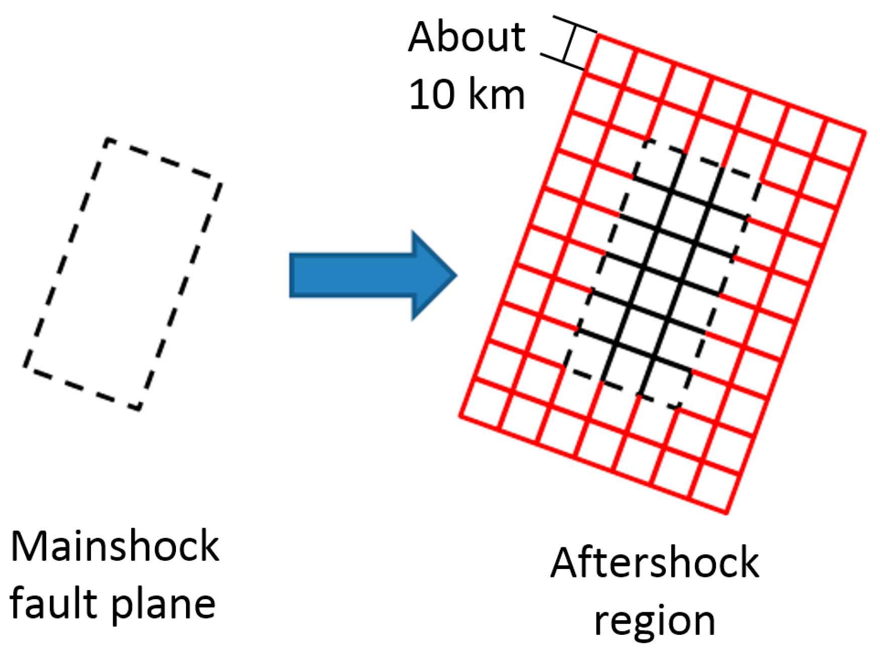
2.1. Aftershock Definition

The classification of aftershocks [11] used in our study is illustrated in Figure 1. In general, many earthquakes subsequently occur near the hypocenter of a large earthquake after its occurrence. If the subsequent earthquakes are smaller in magnitude than the initial earthquake, the initial one is classified as the main shock and the subsequent ones are classified as aftershocks. Conversely, if a subsequent earthquake is larger in magnitude than the initial earthquake, the initial earthquake is classified as a foreshock and the largest subsequent earthquake is classified as the main shock. Typically, subduction earthquakes stronger than a Richter magnitude of 7.0 are assumed to be main shocks because the majority of such earthquakes are historically observed to be main shocks.

The area where the aftershocks occur is the aftershock region, which contains the fault plane as well as the expanded fault plane. The distribution of aftershocks resulting from the Tohoku earthquake as per the Japan Meteorological Agency [12] is depicted in Figure 2. Aftershocks that occur at a large distance from the fault plane, i.e., induced earthquakes (e.g., on 12 March 2011, or 15 March 2011), are not included in this study.

2.2. Probabilistic Aftershock Occurrence Model

2.2.1. Reasenberg and Jones Model

In this study, we assume that the relationship between the magnitude and frequency of aftershocks can be expressed using the Gutenberg–Richter (GR) law [13]. Further, we observe that the relationship between the time elapsed after the main shock and the occurrence of the aftershocks agree with the modified Omori’s (MO) law [14,15,16]. Consequently, Reasenberg and Jones proposed a model that can describe the rate of occurrence of aftershocks with a magnitude greater than or equal to M at a time t immediately after a main shock of magnitude M_m, and this can be expressed as follows [17]:

$$\lambda \left(t,M,M_m\right)=\frac{{10}^{a+b\left(M_m-M\right)}}{{\left(t+c\right)}^p},$$

(1)

where a is proportional to the occurrence of earthquakes, b describes the magnitude distribution of the earthquakes, p is the decay rate of the aftershocks, and c is the time-offset parameter, which is assumed to be a constant of 0.1 in this study.

The total number of aftershocks is calculated by integrating Equation (1):

$$\begin{array}{c}N\left(T_1,M,M_m\right)={{\displaystyle \int }}_0^{T_1}\lambda \left(t,M,M_m\right)dt\\ ={10}^{a+b\left(M_m-M\right)}\frac{{\left(T_1+c\right)}^{1-p}-c^{1-p}}{1-p}\hspace{1em}\left(p\ne 1\right),\end{array}$$

(2)

where T₁ is the elapsed time from the main shock. In Equation (2), the relationship between a and the magnitude of the main shock M_m is not specified. However, it is constant regardless of the elapsed time from the main shock. Therefore, the change in the value of b owing to the elapsed time is not considered.

2.2.2. Proposed Probabilistic Aftershock Occurrence Model

We previously proposed Equation (3) [10], which contains a parameter a as a function of the magnitude of the main shock and a parameter b as a function of the elapsed time from the main shock T₁. In addition, the minimum magnitude of the aftershocks (M_min) is set to 4.0 [10].

$$N\left(T_1,M_{min},M_m\right)={10}^{a\left(M_m\right)+b\left(T_1\right)\left(M_m-M_{min}\right)}\frac{{\left(T_1+c\right)}^{1-p}-c^{1-p}}{1-p}\hspace{1em}\left(p\ne 1\right)$$

(3)

Further, when the probability distribution of the earthquake scale is designed using the GR law, the probability that the aftershock magnitude M becomes m_i at T₁ is

$$\begin{array}{c}P\left(m_i|T_1\right)=P\left(m_i-\Delta m/2\le \mathrm{M}<m_i+\Delta m/2|T_1\right)\\ =\frac{N\left(T_1,m_i-\Delta m/2,M_m\right)-N\left(T_1,m_i+\Delta m/2,M_m\right)}{N\left(T_1,M_{min}-\Delta m/2,M_m\right)-N\left(T_1,M_m+\Delta m/2,M_m\right)},\end{array}$$

(4)

where Δm is assumed to be 0.1. In Equation (3), it is assumed that the maximum aftershock magnitude (M_max) is equal to the main shock magnitude (M_m). However, we propose the following Equation (5) according to previous studies [18,19]. Hereafter, M_m is represented in terms of M_max using Equation (5):

$$M_m=M_{max}+D_1.$$

(5)

2.3. Model Parameters

Historically large earthquakes including the Tohoku earthquake of 2011, the Tokachi–Oki earthquake of 2003, and other such major earthquakes were compiled to construct an aftershock occurrence model for large earthquakes that may occur in the future. We define aftershocks as earthquakes that occur within 90 days [20] in the area ruptured by the main shock with a focal depth shallower than 100 km and a magnitude (M_J) larger than or equal to 4.0. The hypocenter data (time, location, and magnitude) obtained from the Japan Meteorological Agency were used [21,22]. The spatial distribution of the aftershocks is illustrated in Figure 3.

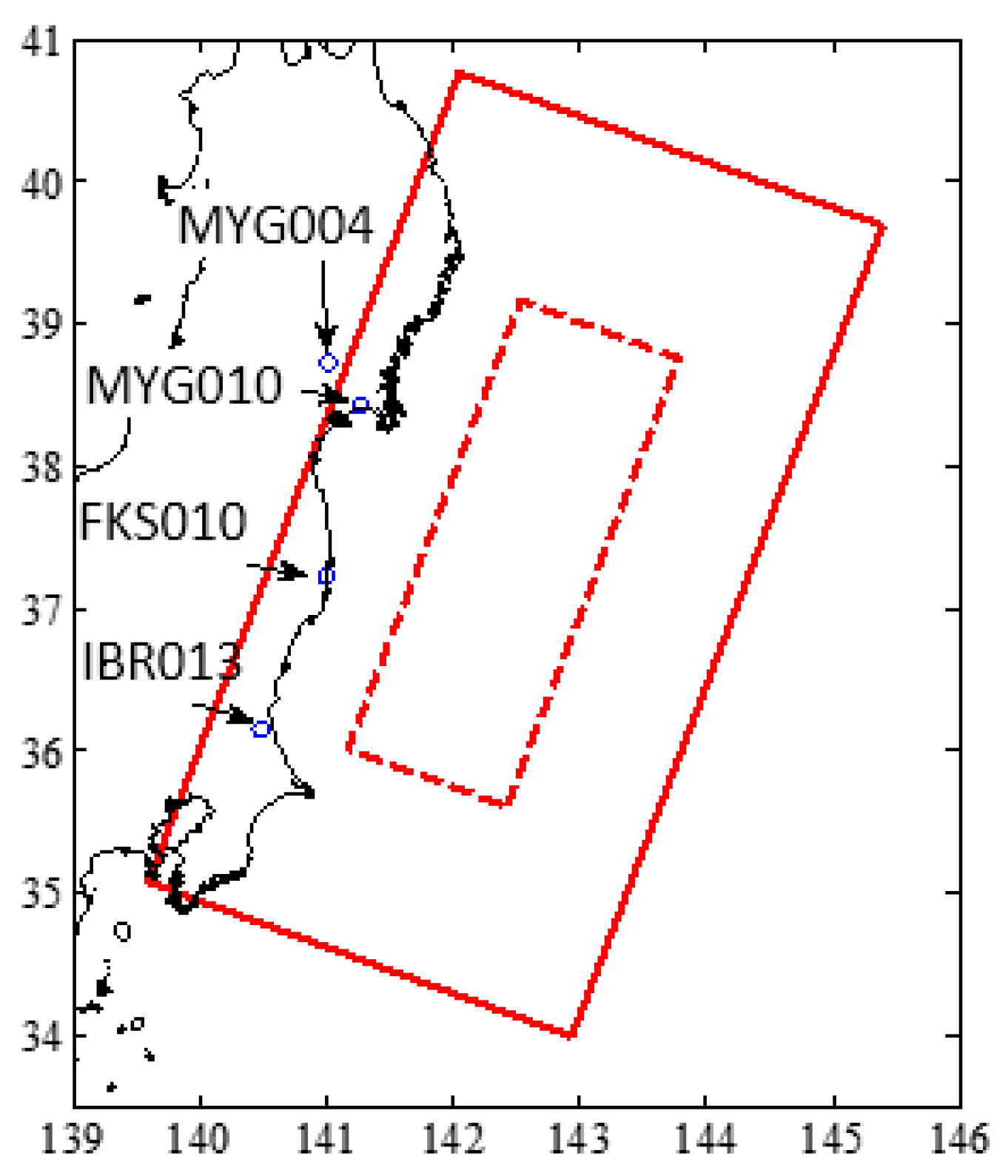
2.3.1. Target Aftershocks

For the 2011 Tohoku earthquake, we used the fault model of the Geospatial Information Authority of Japan [23] to estimate the expanded fault plane, which acts as the aftershock area. For the 2003 Tokachi–Oki earthquake, the Yagi fault model [24] was used to estimate the expanded fault plane. The aftershock areas of other major earthquakes are assumed to be circular regions centered on the hypocenter of the main shock. The aftershock area A (km²) is calculated as follows [20]:

$$lo{g}_{10}A=M_m-3.2$$

(6)

2.3.2. Relationships between Parameters

The parameters of the GR and MO models obtained from the previous aftershock data are depicted in

Table 1. Aftershock occurrence parameters for past earthquakes.

Main Shock				Aftershock Parameters				Reference
Mm	GMT	Longitude	Latitude	N	b(90)	p	D1
9.0	20110311	142.9	38.1	3123	0.99	0.86	1.3
7.0	20080507	141.6	36.2	27	0.91	0.84	1.2
8.0	20030925	144.1	41.8	212	0.84	1.02	0.9
7.3	19951203	150.1	44.6	329	0.89	0.97	0.3
7.2	19950106	142.3	40.2	26	0.7	0.76	1.0
7.6	19941228	143.7	40.4	191	0.8	0.93	1.1
6.9	19920718	143.4	39.4	100	0.8	1.09	0.5
7.1	19891101	143.1	39.9	34	0.74	0.94	0.8
6.7	19870206	141.9	36.9	NA	0.88	0.91	1.1	[25]
7.1	19840806	132.2	32.4	NA	1.03	1.00	2.3	[25]
7.0	19820723	142.0	36.2	49	0.83	0.98	0.8
7.4	19780612	142.2	38.2	30	0.69	0.86	1.1
7.9	19680516	143.6	40.7	NA	0.90	1.00	0.4	[26]
7.5	19640616	139.2	38.4	NA	1.00	1.40	1.4	[26]
7.0	19610226	131.9	31.6	NA	0.75	1.00	1.7	[26]
6.8	19610112	142.3	36.0	NA	0.80	1.30	0.2	[26]
7.5	19600320	143.5	39.8	NA	0.85	1.30	0.8	[26]
8.1	19520304	143.9	42.2	NA	0.80	1.10	1.1	[26]
8.1	19461220	135.6	33.0	NA	0.70	1.00	0.9	[26]
8.0	19441207	136.2	33.7	NA	0.70	1.10	1.3	[26]
7.7	19381105	141.6	37.1	NA	0.65	1.20	0.1	[26]
7.1	19380523	141.4	36.7	NA	0.80	1.10	1.2	[26]
8.3	19330302	144.7	39.1	NA	1.10	1.40	1.6	[26]

, which includes the parameters used in previous studies [25,26]. Figure 4 illustrates the relationship between M_m and each declared parameter. The number of aftershocks (N) increases with increasing M_m. However, we cannot confirm the relationships between the other parameters. We use regression to propose the following equations (average and standard deviation) as the aftershock occurrence model parameters.

$$lo{g}_{10}{A}_{after}=0.778M_m-1.60$$

(7)

$$lo{g}_{10}\overline{\mathrm{N}}\left(90,4.0,M_m\right)=0.88M_m-4.51,\hspace{1em}{\sigma }_{lo{g}_{10}\overline{\mathrm{N}}}=0.36$$

(8)

$$\overline{b}\left(90\right)=0.83,{\sigma }_{b\left(90\right)}=0.12$$

(9)

$$\overline{p}=1.05,{\sigma }_p=0.17$$

(10)

$$\overline{D_1}=1.0,{\sigma }_{D_1}=0.5.$$

(11)

In addition, Figure 5a depicts the GR model at various elapsed times (T₁) of the Tohoku earthquake. The b-value (the slope of the GR equation) increases with increasing elapsed time. Figure 5b illustrates the relationship between elapsed time (T₁) and b(T₁) for major earthquakes in the past. As depicted in Figure 5b, b(T₁) is given by the following equation:

$$\overline{b}\left(T_1\right)=0.068lo{g}_{10}\left(T_1\right)+0.70,{\sigma }_{\overline{b}\left(T_1\right)}=0.12$$

(12)

where N is the number of aftershocks that occurred in the aftershock region within a period of 90 days having a magnitude greater than 4.0 (the results of Guo and Ogata [25] and Utsu [26] were excluded due to their having different conditions than the ones required), b(90) is the b-value of the GR equation 90 days after the occurrence of the main shock, p is the decay rate of the MO law, and D₁ is the magnitude difference between the main shock and the largest aftershock.

3. Aftershock Hazard Analysis Method

3.1. Aftershock Hazard Analysis Equation

Seismic hazard analyses are used to assess the relationship between the expected earthquake ground motion at a certain period of time and the probability or frequency of exceedance. In this study, we concentrate on aftershocks due to large subduction earthquakes. The average number of aftershock occurrences for $T_1$ days with a ground motion intensity (Y_surf) greater than y is [24]

$$N\left(Y_{surf}>y|T_1,M_m\right)=N\left(T_1,M_{min},M_m\right){\displaystyle \sum }_i{\displaystyle \sum }_{j}P\left(Y_{surf}>y|m_i,r_j\right)P\left(m_i|T_1\right)P\left(r_j|m_i\right),$$

(13)

where $N\left(T_1,M_{min},M_m\right)$ is the average number of aftershocks having magnitudes greater than 4.0 within the aftershock region, $P\left(Y_{surf}>y|m_i,r_j\right)$ is the conditional probability of a ground motion intensity ($Y_{surf}$) that is greater than y when the aftershock magnitude is $m_i$ and the distance is $r_j$, $P\left(m_i|T_1\right)$ is the probability function of the aftershock magnitude in the aftershock region at an elapsed time $T_1$, and $P\left(r_j|m_i\right)$ is the probability function of the distance at an aftershock magnitude $m_i$. We assume a uniform probability distribution in the aftershock region. In addition, we use the following attenuation relation [27] to calculate the peak ground velocity (PGV) as the aftershock hazard, which can more stably estimate the structural damage than the peak ground acceleration (PGA):

$$\begin{array}{c}{\log }_{10}{Y}_{bed}=\widehat{b}-{\log }_{10}\left(X+\widehat{c}\right)-0.002X,\\ \widehat{b}=0.58M+0.0038D-0.31+\epsilon ,\\ \widehat{c}=0.0028\times {10}^{0.50M},\end{array}$$

(14)

where $Y_{bed}$ is the PGV (cm/s) on the engineering bedrock, M is the aftershock magnitude, D is the focal depth (km), X is the shortest source distance (km), and ε is the deviation between the observed and predicted values with a logarithm standard deviation of 0.23. X is the distance from a spherical surface of radius 1/2L around the hypocenter and is calculated using Equation (15) in accordance with the study by Utsu [28]. In addition, we set X to 3 km when the distance is shorter than 1/2L.

$${\log }_{10}L=0.5M-1.85$$

(15)

Site effects are calculated using the following equations:

$$Y_{surf}=Y_{bed}\times R,$$

(16)

$${\log }_{10}R=1.83-0.66{\log }_{10}AVS30,$$

(17)

where $Y_{surf}$ is the PGV (cm/s) on the surface, R is the site amplification, and AVS30 (m/s) is the average S-wave velocity down to 30 m.

The aftershock region is assumed to be the expanded fault plane, which is an extension of the fault plane in accordance with Equation (7). We divide the expanded fault plane into a 10 km × 10 km mesh, as shown in Figure 6. The aftershock hazard at each site is calculated by integrating the results of each mesh.

3.2. Verification of the Proposed Method

We calculated the PGV hazard curve for the aftershocks of the Tohoku earthquake to validate the proposed model using the proposed aftershock hazard analysis method. The site location and aftershock region of the model are exhibited in Figure 7 and the site-specific parameters are listed in

Table 2. Aftershock occurrence parameters.

Site (K-NET)	Longitude	Latitude	AVS30 (m/s)
MYG010	141.28	38.43	262
MYG004	141.02	38.73	430
FKS010	141.00	37.23	409
IBR013	140.49	36.16	265

.

3.2.1. Comparison of the Aftershock Hazard Analysis and Observations

We compared the actual observations to the results of the aftershock hazard analysis to validate the proposed model. The aftershock hazard analysis for a period of 90 days after the major shock is calculated by considering the average as well as the average ± one standard deviation of each parameter, and the actual aftershock observation records at each site obtained within 90 days after the main shock are depicted in Figure 8. To compare the aftershock hazard and the main shock PGV, the PGV observations for the main shock are depicted by the dashed line, the points where the aftershock hazard curves and main shock PGVs intersect are checked, and the frequency of exceedance is confirmed. For example, in MYG010, the observations and aftershock hazard analysis are in good agreement. The PGV of the main shock is 56 cm/s. Therefore, the maximum expected aftershock occurrence number within 90 days of the main shock is approximately 0.1 times the average parameter values and approximately 0.5 times the average + one standard deviation. At other sites (MYG004, FKS010, and IBR013), the observations and the aftershock hazard analysis match well at relatively small PGVs but not so well with increasing PGVs. The PGVs of the main shock are 110, 62, and 69 cm/s, whereas the maximum expected aftershocks within 90 days of the main shock are approximately 0.07, 0.4, and 0.4 times the results of the average + one standard deviation, respectively. Therefore, the aftershock hazard analysis matches the observations well using the proposed parameters. However, there are deviations between the expected and observed values. Therefore, we need to evaluate the hazards considering the variations in the parameters.

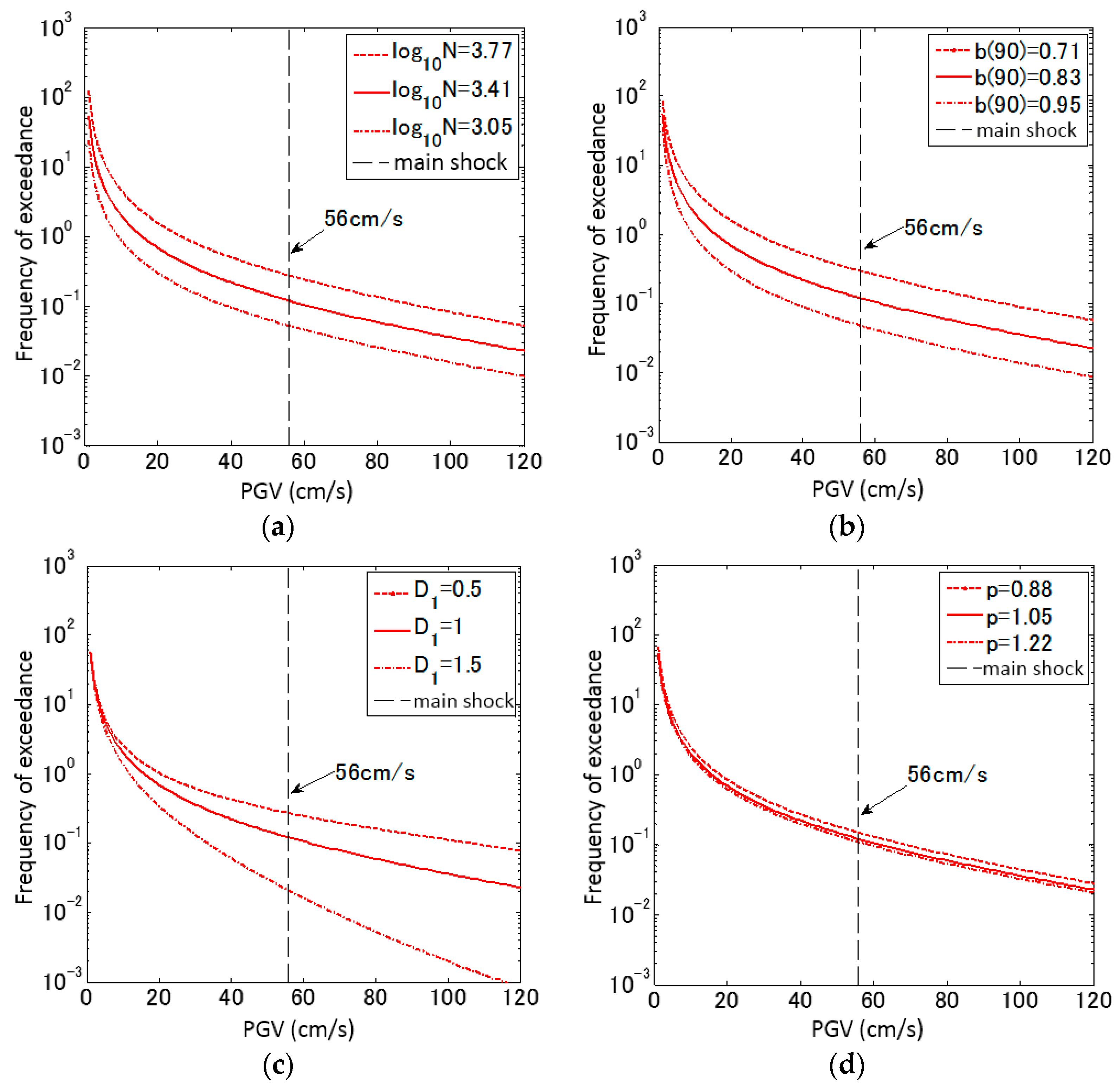
3.2.2. Sensitivity Analysis

As previously mentioned, the parameters used to calculate the aftershock hazards ($lo{g}_{10}N\left(90,4.0,9.0\right)$, b(90), $D_1$, and p) have prediction errors. We performed a sensitivity analysis of these parameters to evaluate the effect of the variations on the accuracy of the analysis. We consider the MYG010 site, using the proposed parameters of Equations (7)–(12), and calculate the aftershock hazards for the average and the average ± one standard deviation of each parameter for 90 days after the earthquake (Figure 9).

The aftershock hazard increases with increasing N-values as well as with decreasing b(90), D₁, and p-values. The contribution of each parameter to the aftershock hazard varies.

3.2.3. Short-Term Versus Mid-Term

We compared the short-term (0–3 days) and mid-term (3–30 days) aftershock hazards at MYG010 (Figure 10) to evaluate the differences in the aftershock hazards owing to the elapsed time from the main shock. The mid-term aftershock hazard is calculated by the following equation:

$$N\left(Y_{surf}>y|3\le t<30,M_m\right)=N\left(Y_{surf}>y|30,M_m\right)-N\left(Y_{surf}>y|3,M_m\right).$$

(18)

We can observe from the mean μ in Figure 10a that the PGVs of the aftershocks that are expected to occur more than once are approximately 18 cm/s in the short-term and approximately 2 cm/s in the mid-term. Figure 10b shows that the maximum expected aftershock occurrence number for μ + σ is 0.6 times in the short-term and nearly 0 times in the mid-term. Therefore, the mid-term hazard is smaller than the short-term hazard; this could be used to estimate the starting time for recovery activities.

4. Engineering Applications

4.1. Aftershock Hazard Map for Recovery Activities

The strong aftershocks that occur after a large subduction earthquake will adversely affect recovery activities [29,30,31]. For example, the gas, water, and electricity supply were disconnected over a wide area owing to an aftershock with a magnitude of 7.2 on 7 April 2011, nearly a month after the Tohoku earthquake. Further, railway facilities and highways were damaged by the strong aftershocks, affecting the train schedules and resulting in a closure of the highways. In addition, it is crucial to decide whether or not to discontinue operations at nuclear facilities. If large aftershocks occur during rescue and lifeline recovery activities after the main shock, there is a further possibility of secondary damages. As explained above, we need to make decisions as per prescribed priorities and implementation plans regarding rescue activities, lifeline recovery activities, and evacuation plans quickly owing to the subsequent aftershocks following a great earthquake. In such a scenario, a framework that can reasonably predict the aftershock activity after a great earthquake is necessary to make such decisions in a timely manner.

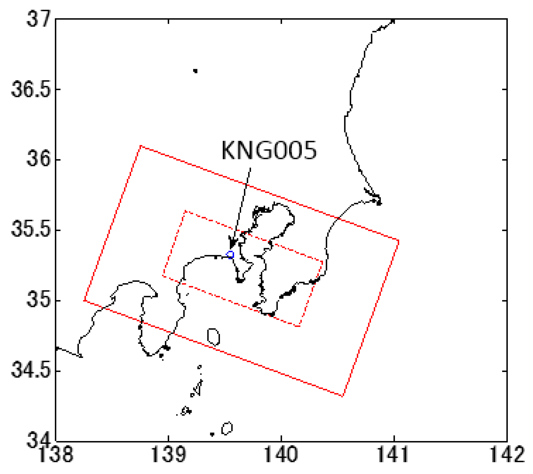
4.1.1. The 1923 Kanto Earthquake

We assume the aftershock hazards for a large earthquake that may occur in the future in the Tokyo metropolitan area [32]. Subsequently, we propose a hazard map using the results of the aftershock hazard analysis for the recovery activities.

Initially, we evaluated the aftershock hazards by applying the proposed model to the Kanto earthquake. The aftershock region is assumed to be the expanded fault plane and the main shock magnitude is in the fault plane [33] (Equation (6)). The main shock magnitude (M_m) is 7.9, the assumed site is KNG005 on K-NET, and the AVS30 of KNG005 is 443 m/s. The site and expanded fault plane are depicted in Figure 11.

Figure 12 illustrates the short-term aftershock hazards and the main shock PGV. The predicted main shock PGV is 48 cm/s, and the maximum aftershock frequency of three days is approximately 0.1 for μ + σ and approximately 0.02 for μ.

4.1.2. Aftershock Hazard Map

We propose a hazard map to efficiently use the aftershock hazard analysis for recovery activities. We focused on the short-term aftershock hazards and calculated the expected aftershock frequency at 113 sites (Figure 13). Figure 13a illustrates the results for μ + σ, whereas Figure 13b illustrates the results for μ. Figure 13 illustrates that the aftershock frequencies of the main shock PGV are considerably larger at sites that are closer to the southwestern area where the depth of the expanded fault plane is shallow. The maximum value is 0.52 for μ + σ and 0.20 for μ. The aftershock hazards increase near the fault plane. However, the increase in the PGV of the main shock is more significant, whereas the aftershock frequencies of the main shock PGV are negligible. In addition, the aftershock hazards, main shock PGV, and the aftershock frequencies are considerably smaller at sites located on the northeast side with the deep expanded fault plane. Conversely, the aftershock hazards are significant at sites located near the southwest side with the shallow expanded fault plane because the main shock PGV is small due to the small distance from the fault plane. As a result, the aftershock frequencies of the main shock PGV in this area are large.

The hazard map can be used to plan evacuation and infrastructure recovery after a large earthquake.

4.1.3. Use of the Aftershock Hazard Map

In this study, we propose a hazard map of the aftershock frequencies beyond the main shock PGV immediately following a large earthquake. However, if the aftershock frequencies following the main shock PGV are sufficiently small after a certain elapsed time after the main shock, it is possible to use hazard maps based on various indices. An example would be the standard seismic intensity, which is adopted by specific applications and can be applied to various decision-making situations, including rescue activities, evacuations, lifeline recoveries, nuclear facility operations, and traffic stops by setting the evaluation period to suit the intended use.

4.2. Load Combination of Aftershock and Tsunami for Tsunami-Resistant Designs

Immediately after the main shock of the 2011 Tohoku earthquake, many structures along the coast of the Tohoku region collapsed due to the simultaneous effect of the tsunami and the strong ground motions of the aftershocks. Even though the primary cause of the collapses of the structures was considered to be the tsunami load, the influence of the strong ground motions of the main shock and aftershocks cannot be ignored. In particular, critical structures, such as tsunami refuge buildings, seawalls, and nuclear power plants, which are located on the seashore, must be designed to withstand tsunamis and strong ground motions. It is necessary to quantitatively evaluate and consider the effects of load combinations of aftershock and tsunami. Even if the seismic design and tsunami-resistant design are appropriate, they may not account for the simultaneous occurrence of both aftershocks and tsunamis. In tsunami-resistant designs, we need to expect tsunamis to arrive at any time after the main shock ranging from a few minutes to a few hours based on the experience of the Tohoku earthquake. Therefore, both aftershocks and tsunamis should be considered simultaneously to design critical facilities located at the seashore. A practical assessment of the combined load of aftershocks and tsunamis is needed if both aftershocks and tsunamis occur simultaneously.

4.2.1. Load Combination Framework

The concept of the simultaneous occurrence of aftershocks and tsunamis [34] is depicted in Figure 14. Initially, the maximum tsunami arrival time at the evaluation site is expressed as the elapsed time t_a and the tsunami completion time is expressed as t_e from the time of occurrence of the main shock. Therefore, the tsunami duration is represented as t_e − t_a. According to the analysis of the Tohoku earthquake, t_a was short and t_e − t_a was a few minutes. Conversely, the load effects of the aftershocks occur immediately after the main shock and simultaneous effects of the aftershocks and the tsunami on structures occur within t_e − t_a. Therefore, we propose the use of load and resistance combination factors in tsunami-resistant designs. The maximum height of the tsunami will arrive at the specified site at time t_a after the main shock, and the maximum value is continuous within the tsunami duration and will be combined with the maximum value of the aftershock loads during the tsunami duration.

4.2.2. Analytical Model and Conditions

To evaluate the load combination factors of aftershocks and tsunamis in the Tohoku region, we assumed the main shocks to be the 2011 Tohoku earthquake (M_m = 9.0), the 1933 Sanriku earthquake (M_m = 8.1), and the 1896 Sanriku earthquake (M_m = 8.5). The evaluation sites are the K-NET locations of AOM012, IWT001, IWT002, IWT003, IWT005, and IWT007. The aftershock area is the expanded fault plane, which is enlarged due to the relationship between the main shock magnitude and the aftershock area [35]. The evaluation sites and aftershock area are depicted in Figure 15.

The target structure is a ten-story reinforced concrete structure, with a width of 40 m, a depth of 20 m, and a height of 40 m. Based on the experience of the Tohoku earthquake [36], t_a is set to 0 min, 30 min, and 60 min after the main shock and the tsunami duration is set to 30 min. The inundation height is assumed to remain constant during the entire duration of the tsunami. The limiting state is that in which the horizontal load of the aftershocks and the tsunami exceed the lateral resistance of the structure.

The design equation for the limiting state function [37] is

$$\phi R_n>{\gamma }_A{Q}_{An}+{\gamma }_T{Q}_{Tn}={\gamma }_A(r{Q}_{Mn})+{\gamma }_T{Q}_{Tn}={\gamma }_M{Q}_{Mn}+{\gamma }_T{Q}_{Tn},$$

(19)

where Q_An is the conditional representative value of the aftershock load during the tsunami duration under the specified occurrence of the main shock, which we assume is a mean value based on the aftershock hazard analysis; Q_Tn is the conditional representative value of the tsunami load under the specified occurrence of the main shock, which we assume is the mean value estimated based on the Abe law [38]; Q_Mn is the conditional representative value of the main shock load under the specified occurrence of the main shock, which we assume is the median value estimated from the attenuation relation [27]; R_n is the nominal value of the lateral resistance; γ_A is the load factor for the aftershocks; γ_T is the load factor for the tsunami; γ_M is the load factor for the aftershocks; $\phi$ is the resistance factor; and r = Q_An/Q_Mn is the ratio of the nominal value of the load effect owing to aftershocks during the tsunami duration to the nominal value of the load effect owing to the main shock.

• Aftershock load

First, we design the load effect of the aftershocks. We focus on the horizontal base shear force of n-story structures. According to the Recommendations for Loads on Buildings [39], the seismic base shear force Q_A is approximately 2 times that of the ground seismic response:

$$Q_A\approx \frac{2PGA}{g}{\displaystyle \sum }_{k=1}^n{w}_k,$$

(20)

where w_k is the weight of the floor k (kN), g is the gravitational acceleration [m/s²], n is the number of stories of the target building, and PGA is the peak ground acceleration owing to the aftershocks [m/s²], which is a random variable determined using Equation (13). Note that PGA is used instead of PGV. Therefore, we use the following attenuation relations (Equation (21)) for the calculation of PGA as an aftershock hazard and the site amplification R is assumed to be 1.4.

$$\begin{array}{c}{\log }_{10}{Y}_{bed}=\widehat{b}-{\log }_{10}\left(X+\widehat{c}\right)-0.003X\\ \widehat{b}=0.50M+0.0043D+0.62+\epsilon \\ \widehat{c}=0.0055\times {10}^{0.50M}\end{array}$$

(21)

We use σ to model the error of the earthquakes. The mean (μ) and μ + σ of the aftershock PGA at each evaluation site are summarized in

Table 3. Summary of the input values in the reliability analysis.

Sites	Variable	2011 Tohoku		1896 Sanriku		1933 Sanriku		Type	Note
		Mean	COV	Mean	COV	Mean	COV
AOM012	PGA0–30 (cm/s2)	83	1.61	68.2	1.37	11.7	1.13	Lognormal	μ
		185	1.35	140	1.25	22.2	1.05	Lognormal	μ + σ
	PGA30–60 (cm/s2)	62	1.73	53.5	1.46	9.5	1.20	Lognormal	μ
		135	1.50	107	1.35	17.8	1.11	Lognormal	μ + σ
	PGA60–90 (cm/s2)	53	1.81	46.3	1.52	8.4	1.25	Lognormal	μ
		113	1.59	91.8	1.41	15.5	1.16	Lognormal	μ + σ
	PGAmain (cm/s2)	176	-	238	-	93	-	-	Median
	h (m)	9.6	0.42	3.7	0.42	1.2	0.42	Lognormal
	R (kN)	-	0.2	-	0.2	-	0.2	Lognormal
IWT001	PGA0–30 (cm/s2)	106	1.58	81.3	1.36	14.8	1.12	Lognormal	μ
		234	1.28	166	1.22	28.2	1.05	Lognormal	μ + σ
	PGA30–60 (cm/s2)	79	1.71	63.8	1.45	12.1	1.19	Lognormal	μ
		171	1.43	128	1.31	22.5	1.11	Lognormal	μ + σ
	PGA60–90 (cm/s2)	67	1.79	55.1	1.51	10.6	1.25	Lognormal	μ
		143	1.52	109	1.38	19.7	1.16	Lognormal	μ + σ
	PGAmain (cm/s2)	215	-	283	-	118	-	-	Median
	h (m)	10.3	0.42	4.1	0.42	1.3	0.42	Lognormal
	R (kN)	-	0.2	-	0.2	-	0.2	Lognormal
IWT002	PGA0–30 (cm/s2)	125	1.52	76.7	1.34	16.6	1.11	Lognormal	μ
		274	1.21	157	1.21	31.6	1.03	Lognormal	μ + σ
	PGA30–60 (cm/s2)	94	1.65	60.2	1.42	13.5	1.18	Lognormal	μ
		201	1.35	120	1.31	25.3	1.10	Lognormal	μ + σ
	PGA60–90 (cm/s2)	79	1.73	52.1	1.48	11.9	1.23	Lognormal	μ
		168	1.44	103	1.37	22	1.14	Lognormal	μ + σ
	PGAmain (cm/s2)	270	-	262	-	126	-	-	Median
	h (m)	11.3	0.42	4.3	0.42	1.4	0.42	Lognormal
	R (kN)	-	0.2	-	0.2	-	0.2	Lognormal
IWT003	PGA0–30 (cm/s2)	146	1.52	78.8	1.33	19.3	1.09	Lognormal	μ
		322	1.20	161	1.21	36.6	1.02	Lognormal	μ + σ
	PGA30–60 (cm/s2)	108	1.65	61.9	1.42	15.7	1.16	Lognormal	μ
		235	1.35	123	1.30	29.3	1.08	Lognormal	μ + σ
	PGA60–90 (cm/s2)	92	1.74	53.5	1.48	13.8	1.21	Lognormal	μ
		197	1.44	106	1.36	25.6	1.13	Lognormal	μ + σ
	PGAmain (cm/s2)	336	-	268	-	141	-	-	Median
	h (m)	12.4	0.42	4.7	0.42	1.5	0.42	Lognormal
	R (kN)	-	0.2	-	0.2	-	0.2	Lognormal
IWT005	PGA0–30 (cm/s2)	167	1.38	69.8	1.31	21.5	1.07	Lognormal	μ
		358	1.07	142.2	1.21	40.7	0.99	Lognormal	μ + σ
	PGA30–60 (cm/s2)	125	1.51	54.9	1.40	17.5	1.14	Lognormal	μ
		265	1.21	109.3	1.30	32.6	1.06	Lognormal	μ + σ
	PGA60–90 (cm/s2)	106	1.59	47.5	1.46	15.4	1.19	Lognormal	μ
		223	1.30	93.7	1.36	28.5	1.11	Lognormal	μ + σ
	PGAmain (cm/s2)	469	-	234	-	148	-	-	Median
	h (m)	15.0	0.42	5.0	0.42	1.6	0.42	Lognormal
	R (kN)	-	0.2	-	0.2	-	0.2	Lognormal
IWT007	PGA0–30 (cm/s2)	174	1.35	52.7	1.27	20	1.06	Lognormal	μ
		373	1.05	107	1.20	37.9	0.99	Lognormal	μ + σ
	PGA30–60 (cm/s2)	130	1.49	41.5	1.36	16.3	1.13	Lognormal	μ
		276	1.18	82.5	1.29	30.4	1.05	Lognormal	μ + σ
	PGA60–90 (cm/s2)	111	1.54	35.9	1.42	14.3	1.18	Lognormal	μ
		232	1.27	70.8	1.35	26.5	1.10	Lognormal	μ + σ
	PGAmain (cm/s2)	533	-	179	-	134	-	-	Median
	h (m)	18.1	0.42	4.8	0.42	1.5	0.42	Lognormal
	R (kN)	-	0.2	-	0.2	-	0.2	Lognormal

. In addition, the PGA distribution type is assumed to be lognormal.

• Tsunami load

Next, according to the tsunami-resistant design [40], the tsunami load Q_T is

$$Q_T=\gamma B{{\displaystyle \int }}_{z_1}^{z_2}\left(3h-z\right)dz=\frac{1}{2}\gamma B\left\{\left(6h{z}_2-z_2{}^2\right)-\left(6h{z}_1-z_1{}^2\right)\right\},$$

(22)

where B is the width of the target structure [m], γ is the specific weight of water (kN/m³), z₁ is the minimum height of the tsunami pressure-receiving surface ($0\le z_1\le z_2$) (m), z₂ is the maximum height of the tsunami pressure-receiving surface ($z_1\le z_2\le 3h$) (m), and h is the design tsunami inundation depth (m).

The mean value of the design tsunami inundation depth is calculated by assuming a lognormal distribution for h and a standard deviation equal to 0.42 [38,41]:

$${\log }_{10}\overline{h}=M_m-{\log }_{10}\Delta -5.55+\mathrm{C},$$

(23)

where $\overline{h}$ is the mean value of the design tsunami inundation depth [m], M_m is the main shock magnitude, $\Delta$ is the shortest tsunami propagation distance from the hypocenter to the observation point [km], and C is a correction term that is 0 toward the Pacific Ocean and 0.2 toward the Japan Sea.

• Load-resistance capacity

The mean load-resistance capacity, R_n is estimated using a target reliability index. Its coefficient of variation (COV) is assumed to be 0.2, and its distribution is assumed to be lognormal.

4.2.3. Analytical Method

The advanced first-order second moment (AFOSM) [42] is used as the method for the analysis. In this study, β_T is the conditional target reliability index under the specified main shock occurrence. Therefore, it is necessary to determine β_T by considering the occurrence frequency of the main shock. According to the Headquarters for Earthquake Research Promotion [43], the return period of the Tohoku earthquake is 600 years and that of the Sanriku earthquake is 97 years. Therefore, we set the conditional target reliability index β_T to take values from 0.0 to 1.0 and calculated the design value of the aftershock and tsunami load combination. In addition, the load combination factor was estimated from the ratio of the representative and design values.

4.3. Results

4.3.1. Analytical Results

Figure 16 illustrates the aftershock and tsunami load combination factor at IWT007, whereas Figure 17 depicts the results at all the evaluation sites.

According to Figure 16, regardless of the main shock, the tsunami load factor increases with increasing target reliability index. However, the aftershock load factor remains nearly constant, and the resistance factor decreases. The aftershock load factor tends to decrease with increasing elapsed time from the main shock. The difference between 30–60 min and 60–90 min is smaller than that between 0–30 min and 30–60 min because the occurrence rate of the aftershocks decreases with increasing elapsed time. However, the effect of the elapsed time on the tsunami load factor and the resistance factor is negligible.

Figure 16a,c,e are compared to Figure 16b,d,f to confirm the effect of variations in the aftershock hazard analysis. The variation is significant in the aftershock load factor, which was approximately three times the variation. Simultaneously, we compared the 2011 Tohoku earthquake (M_m = 9.0), the 1896 Sanriku earthquake (M_m = 8.5), and the 1933 Sanriku earthquake (M_m = 8.1) to confirm the effect of the magnitude of the main shock. It is difficult to make a direct comparison because the shortest distance from an evaluation site to the fault plane is different at different sites. The aftershock load factor and tsunami load factor of the 1933 Sanriku earthquake were affected negligibly compared to the factors for the 2011 Tohoku and 1896 Sanriku earthquakes. In addition, the aftershock load factor decreases and the tsunami load factor increases with increasing elapsed time after the main shock. The variation in the tsunami load factor for the 1933 Sanriku earthquake is remarkable. The main shock magnitude of the 1933 Sanriku earthquake is the smallest of the target earthquakes. Therefore, the load effect of the tsunami is considerably smaller than the load effect of the aftershocks.

Here, we summarize the results at all the evaluation sites. The relationship between the fault distance and the load combination factor for the target reliability index is illustrated in Figure 17. The aftershock load factor and the tsunami load factor for each target reliability index are set high and the resistance factor is set low to evaluate the most conservative load combination factor, including the effects of elapsed time. Figure 16 indicates that the load combination factors are nearly constant regardless of the fault distance. However, the aftershock load factor for the 1933 Sanriku earthquake is the smallest of the three earthquakes. This is because the aftershock occurrence rate is related to the main shock magnitude. Conversely, the resistance factor is nearly constant regardless of the main shock magnitude. Moreover, the aftershock load factor increases when the aftershock hazard increases owing to the variation. However, there is little change in the tsunami load factor owing to the variation in the aftershock hazard for the 2011 Tohoku earthquake and the tsunami load factor decreases with increasing aftershock hazard for the 1896 and 1933 Sanriku earthquakes. Presumably, this is because the tsunami to aftershock load ratios in the 1896 and 1933 Sanriku earthquakes are smaller than that of the 2011 Tohoku earthquake.

4.3.2. Load Combination Factor for Tsunami-resistant Designs

We consider the very rare condition that large subduction earthquakes (Tohoku and Sanriku earthquakes) occur. Therefore, the conditional target reliability index is set to 0 and 0.5. The LRFD format for the tsunami-resistant design of the conditional target reliability index is shown in

Table 4. Summary of the load and resistance factor design factor.

Magnitude of Main Shock (Mm)	Conditional Target Reliability						Note
	Index = 0			Index = 0.5
	$\mathit{\phi }$	${\mathit{\gamma }}_{\mathit{M}}$	${\mathit{\gamma }}_{\mathit{T}}$	$\mathit{\phi }$	${\mathit{\gamma }}_{\mathit{M}}$	${\mathit{\gamma }}_{\mathit{T}}$
9.0	0.98	0.14	0.88	0.95	0.15	1.26	$\mu$
	0.98	0.41	0.88	0.95	0.49	1.25	$\mu +\sigma$
8.5	0.98	0.11	0.86	0.95	0.15	1.25	$\mu$
	0.98	0.25	0.86	0.95	0.47	1.24	$\mu +\sigma$
8.1	0.98	0.06	0.87	0.95	0.10	1.19	$\mu$
	0.98	0.11	0.87	0.95	0.24	1.08	$\mu +\sigma$

.

5. Conclusions

In this study, we introduced a probabilistic aftershock hazard analysis that is expected to be useful to develop plans for recovery activities after any large earthquake in the future. The probabilistic aftershock hazard analysis depends on the elapsed time after the main shock using model parameters based on compiled statistics of historical aftershock data. The proposed model was validated by comparing the results with observed aftershock ground motions during the 2011 Tohoku earthquake. In addition, we conducted a sensitivity analysis and confirmed the effects of variations in each parameter. Then, two engineering applications of the proposed approach for probabilistic aftershock hazard analysis were shown for demonstration purposes. It was proposed that aftershock hazard maps be used for the effective planning of the recovery activity for future large earthquakes that may occur in Japan. It was also proposed that aftershock hazard analysis be used for the development of load combination equations of LRFD considering the simultaneous occurrence of tsunamis and aftershocks, which is considered to be useful for the design of tsunami evacuation buildings.

In the future, we will consider the effects of aftershocks for safety evaluations of nuclear facilities to contribute to the advancement of probabilistic seismic risk analyses of nuclear facilities.

References

1. The Central Disaster Management Council: Committee for Policy Planning on Disaster Management. Available online: http://www.bousai.go.jp/en/documentation/reports/disaster_management_plan.html (accessed on 10 October 2017).
2. Yeo, G.L.; Cornell, C.A. A probabilistic framework for quantification of aftershock ground-motion hazard in California: Methodology and parametric study. Earthq. Eng. Struct. Dyn. 2009, 38, 45–60. [Google Scholar] [CrossRef]
3. Gerstenberger, M.C.; Wiemer, S.; Jones, L.M.; Resenberg, P.A. Real-time forecasts of tomorrow’s earthquakes in California. Nature 2005, 435, 328–331. [Google Scholar] [CrossRef] [PubMed]
4. Dan, K.; Okada, Y.; Hanamura, M.; Watanabe, T. Occurrence models of main-shock and aftershocks and their application to time-series simulation of strong ground motions and seismic hazard analysis. In Proceedings of the 12th Japan Earthquake Engineering Symposium, Tokyo, Japan, 3–5 November 2006. [Google Scholar]
5. Miyakoshi, J.; Shimazu, N.; Ju, D.; Kambara, H.; Yamamoto, H. Prediction of building damage considering main shock and aftershocks. In Proceedings of the Annual Meeting of Architectural Institute of Japan, Toyama, Japan, 9–11 September 2010. [Google Scholar]
6. Kumitani, S.; Takada, T. Probabilistic assessment of building damage considering aftershocks of earthquakes. Int. J. Eng. Uncertain. Hazard. Assess. Mitig. 2009, 1, 183–187. [Google Scholar] [CrossRef]
7. Hirose, M.; Itoi, T.; Takada, T. Empirical prediction model for ground motion intensity due to aftershocks. In Proceedings of the 11th International Conference on Structural Safety and Reliability, New York, NY, USA, 16–20 June 2013. [Google Scholar]
8. The Headquarters for Earthquake Research Promotion: Aftershock Probability Evaluation Promotion. (In Japanese). Available online: http://www.jishin.go.jp/reports/research_report/aftershock/main_yoshin2/ (accessed on 12 December 2017).
9. The 2011 Great East Japan Earthquake: First Report. Available online: http://www.jma.go.jp/jma/en/News/2011_Earthquake_01.html (accessed on 10 October 2017).
10. Choi, B.; Itoi, T.; Takada, T. Probabilistic aftershock occurrence model and hazard assessment for post-earthquake restoration activity plan. J. Struct. Constr. Eng. 2013, 78, 1377–1383. (In Japanese) [Google Scholar] [CrossRef]
11. Choi, B.; Takada, T.; Itoi, T. Probabilistic aftershock hazard analysis based on 2011 Tohoku earthquake data. In Proceedings of the 11th International Conference on Structural Safety and Reliability, New York, NY, USA, 16–20 June 2013. [Google Scholar]
12. Aftershocks of the Past Massive Earthquakes. Available online: http://www.eri.u-tokyo.ac.jp/PREV_HP/outreach/eqvolc/201103_tohoku/eng/aftershocksofpast/ (accessed on 30 October 2017).
13. Gutenberg, B.; Richter, C.F. Frequency of earthquakes in California. Bull. Seism. Soc. Am. 1944, 34, 185–188. [Google Scholar]
14. Utsu, T. Some problems of the distribution of earthquakes in time (part 1). Geophys. Bull. Hokkaido. Univ. 1969, 22, 73–93. [Google Scholar]
15. Mignan, A. Modeling aftershocks as a stretched exponential relaxation. Geophys. Res. Lett. 2015, 42, 9726–9732. [Google Scholar] [CrossRef]
16. Kossobokov, V.G.; Nekrasova, A.K. Characterizing aftershock sequences of the recent strong earthquakes in Central Italy. Pure. Appl. Geophys. 2017, 174, 3713–3723. [Google Scholar] [CrossRef]
17. Reasenberg, P.A.; Jones, L.M. Earthquake hazard after a mainshock in California. Science 1989, 243, 1173–1176. [Google Scholar] [CrossRef] [PubMed]
18. Utsu, T. Seismicity Studies: A Comprehensive Review; University of Tokyo Press: Tokyo, Japan, 1999; p. 876. [Google Scholar]
19. Bath, M. Lateral inhomogeneities in the upper mantle. Tectonophysics 1965, 2, 483–514. [Google Scholar] [CrossRef]
20. National Research Institute for Earth Science and Disaster Prevention. A Study on Probabilistic Hazard Maps of Japan; No. 275; National Research Institute for Earth Science and Disaster Resilience: Tokyo, Japan, 2005. [Google Scholar]
21. National Research Institute for Earth Science and Disaster Prevention, Japan. JMA Earthquake List. Available online: http://www.hinet.bosai.go.jp/REGS/JMA/list/ (accessed on 12 March 2012).
22. Japan Meteorological Agency. The Annual Seismological Bulletin of Japan for 2009; Japan Meteorological Agency: Tokyo, Japan, 2009.
23. The 2011 off Pacific coast of Tohoku Earthquake on March 11, 2011: Fault model. Available online: http://www.gsi.go.jp/cais/topic110422-index.html (accessed on 10 October 2017).
24. Yagi, Y. Source rupture process of the 2003 Tokachioki earth-quake determined by joint inversion of teleseismic body wave and strong ground motion data. Earth Planets Space 2004, 56, 311–316. [Google Scholar] [CrossRef]
25. Guo, Z.; Ogata, Y. Statistical relations between the parameters aftershocks in time, space and magnitude. J. Geophys. Res. 1997, 102, 2867–2873. [Google Scholar] [CrossRef]
26. Utsu, T. Aftershocks and earthquake statistics (1). J. Fac. Sci. Hokkaido Univ. 1968, 7, 129–195. [Google Scholar]
27. Si, H.; Midorikawa, S. Attenuation relations for peak ground acceleration and velocity considering effects of fault type and site condition. J. Struct. Constr. Eng. 1999, 523, 63–70. (In Japanese) [Google Scholar] [CrossRef]
28. Utsu, T. Seismology, 3rd ed.; kyoritsu Shuppan: Tokyo, Japan, 2005. (In Japanese) [Google Scholar]
29. Polese, M.; Ludovico, M.D.; Prota, A.; Manfredi, G. Damage-dependent vulnerability curves for existing buildings. Earthq. Eng Struct. Dyn. 2013, 42, 853–870. [Google Scholar] [CrossRef]
30. Iervolino, L.; Giorgio, M.; Chioccarelli, E. Closed-form aftershock reliability of damage-cumulating elastic-perfectly-plastic systems. Earthq. Eng Struct. Dyn. 2014, 43, 613–625. [Google Scholar] [CrossRef]
31. Mignan, A.; Danciu, L.; Giardini, D. Considering large earthquake clustering in seismic risk analysis. Nat. Hazards 2016, 1–24. [Google Scholar] [CrossRef]
32. Choi, B. Methodology Development and Engineering Application of Probabilistic Aftershock Hazard Analysis. Ph.D. Thesis, The University of Tokyo, Tokyo, Japan, March 2014. [Google Scholar]
33. Kobayashi, R.; Koketsu, K. Source process of the 1923 Kanto earthquake inferred from historical geodetic, teleseismic, and strong motion data. Earth Planets Space 2005, 57, 261–270. [Google Scholar] [CrossRef]
34. Choi, B.; Nishida, A.; Itoi, T.; Takada, T. Load combination of aftershocks and tsunami for tsunami-resistant design. In Proceedings of the 12th International Conference on Applications of Statistics and Probability in Civil Engineering, Vancouver, BC, Canada, 12–15 July 2015. [Google Scholar]
35. Sato, R. Handbook of Fault Parameters for Japanese Earthquakes; Kajima Institute Publishing: Tokyo, Japan, 1989. (In Japanese) [Google Scholar]
36. Port and Airport Research Institute. Survey Results. Available online: http://www.pari.go.jp/info/tohoku-eq/20110328mlit.html (accessed on 10 October 2017).
37. American Institute of Steel Construction. AISC Manual of Steel Construction: Load and Resistance Factor Design, 3rd ed.; AISC Manual Committee: Chicago, IL, USA, 2001. [Google Scholar]
38. Abe, K. Estimation of tsunami heights from magnitudes of earthquake and tsunami. Bull. Earthq. Res. Inst. Tokyo Univ. 1989, 64, 51–69. [Google Scholar]
39. Architectural Institute of Japan. Recommendations for Loads on Buildings; Architectural Institute of Japan: Tokyo, Japan, 2004. (In Japanese) [Google Scholar]
40. Okada, T.; Sugano, T.; Ishikawa, T.; Ogi, T.; Takai, S.; Hamabe, T. Structural Design Method of Building to Seismic Sea Wave, No. 2 Design Method (a Draft). Build. Lett. 2004, pp. 1–8. (In Japanese). . Available online: http://www.bousai.go.jp/kohou/oshirase/h16/041220/pdf/siryou_43.pdf (accessed on 19 December 2017).
41. Aida, I. Reliability of a tsunami source model derived from fault parameters. J. Phys. Earth 1978, 26, 57–73. [Google Scholar] [CrossRef]
42. Hoshiya, M.; Ishii, K. The Reliability Designing of Structures; Kajima Institute Publishing: Tokyo, Japan, 1986. (In Japanese) [Google Scholar]
43. The Headquarters for Earthquake Research Promotion. Long-term Evaluation. Available online: http://www.jishin.go.jp/main/choukihyoka/kaikou.htm (accessed on 10 October 2017).
Figure 1. Aftershock classification.
Geosciences 08 00001 g001
Figure 2. Aftershock distribution due to the 2011 Tohoku earthquake.
Geosciences 08 00001 g002
Figure 3. Aftershock distribution for (a) the 2011 Tohoku and 2003 Tokachi–Oki earthquakes (dotted line: fault plane, solid line: expanded fault plane) and (b) other earthquakes.
Geosciences 08 00001 g003
Figure 4. Relationship between Mm and (a) the aftershock area; (b) the number of aftershocks (N); (c) the b-value after 90 days; (d) the p-value; and (e) the D1-value.
Geosciences 08 00001 g004
Figure 5. (a) Gutenberg–Richter (GR) model at different elapsed times (T1) for the 2011 Tohoku earthquake and (b) b(T1) versus T1 for past major earthquakes.
Geosciences 08 00001 g005
Figure 6. Setting of the aftershock region.
Geosciences 08 00001 g006
Figure 7. Site and aftershock region.
Geosciences 08 00001 g007
Figure 8. Aftershock hazard and observations within 90 days of the main shock: (a) MYG010; (b) MYG004; (c) FKS010; and (d) IBR013.
Geosciences 08 00001 g008
Figure 9. Results of a sensitivity analysis of the parameters within 90 days of an earthquake: (a) l o g 10 N ( 90 , 4.0 , 9.0 ) ; (b) b(90); (c) D1, and (d) p.
Geosciences 08 00001 g009
Figure 10. Short-term (0–3 days) and mid-term (3–30 days) aftershock hazard at MYG010: (a) frequency of exceedance equal to 1 and (b) peak ground velocity (PGV) of the main shock.
Geosciences 08 00001 g010
Figure 11. Site and aftershock region of the 1923 Kanto earthquake.
Geosciences 08 00001 g011
Figure 12. Short-term aftershock hazard results at KNG005.
Geosciences 08 00001 g012
Figure 13. Hazard map of the short-term aftershock frequency of the main shock PGV: (a) μ + σ and (b) μ.
Geosciences 08 00001 g013
Figure 14. Concept of aftershock and tsunami load combination.
Geosciences 08 00001 g014
Figure 15. Evaluation sites and the aftershock area.
Geosciences 08 00001 g015
Figure 16. Aftershock and tsunami load combination factor (IWT007) for the (a) 2011 Tohoku (μ); (b) 2011 Tohoku (μ + σ); (c) 1896 Sanriku (μ); (d) 1896 Sanriku (μ + σ); (e) 1933 Sanriku (μ); and (f) 1933 Sanriku (μ + σ) earthquakes.
Geosciences 08 00001 g016
Figure 17. Relationship between the fault distance and the load combination factors: (a) aftershock load factor (βT = 0.0); (b) aftershock load factor (βT = 0.5); (c) tsunami load factor (βT = 0.0); (d) tsunami load factor (βT = 0.5); (e) resistance factor (βT = 0.0); and (f) resistance load factor (βT = 0.5).
Geosciences 08 00001 g017