Realistic Paleobathymetry of the Cenomanian–Turonian (94 Ma) Boundary Global Ocean


1
Department of Natural Sciences, Northwest Missouri State University, Maryville, MO 64468, USA
2
Department of Atmospheric, Oceanic, and Earth Sciences, George Mason University, Fairfax, VA 22030, USA
3
Earth & Planetary Sciences, Johns Hopkins University; Baltimore, MD 21218, USA
*
Author to whom correspondence should be addressed.
Geosciences 2018, 8(1), 21; https://doi.org/10.3390/geosciences8010021
Submission received: 6 November 2017
/
Revised: 5 January 2018
/
Accepted: 10 January 2018
/
Published: 15 January 2018
(This article belongs to the Special Issue Marine Geomorphometry)
Abstract
:At present, global paleoclimate simulations are prepared with bathtub-like, flat, featureless and steep walled ocean bathymetry, which is neither realistic nor suitable. In this article, we present the first enhanced version of a reconstructed paleobathymetry for Cenomanian–Turonian (94 Ma) time in a 0.1° × 0.1° resolution, that is both realistic and suitable for use in paleo-climate studies. This reconstruction is an extrapolation of a parameterized modern ocean bathymetry that combines simple geophysical models (standard plate cooling model for the oceanic lithosphere) based on ocean crustal age, global modern oceanic sediment thicknesses, and generalized shelf-slope-rise structures calibrated from a published global relief model of the modern world (ETOPO1) at active and passive continental margins. The base version of this Cenomanian–Turonian paleobathymetry reconstruction is then updated with known submarine large igneous provinces, plateaus, and seamounts to minimize the difference between the reconstructed paleobathymetry and the real bathymetry that once existed.
1. Introduction
Understanding past climate is critical for the scientific study of ancient, modern, and future climate change. Computer-generated models, also known as general circulation models (GCMs) are often used to study the plausible dynamic effects of diverse boundary conditions on climate. Paleoclimate data provide a useful framework from which these models can be used to predict past, present, and future climate change scenarios. The use of numerical models to investigate Earth’s climate history has increased significantly over the past decade [1,2,3]. These models have grown in sophistication, with increased space–time resolution, coupled ocean-atmosphere GCMs that incorporate vegetation, soil (weathering), ice, and chemistry modules.
Accordingly, more robust and detailed boundary conditions are needed. One of the most difficult and often overwhelming tasks in paleoclimate modeling is the assembly of surface boundary conditions for past time periods [2]. These boundary conditions include but are not limited to continental configurations, topography, ocean bathymetry, ocean chemistry, terrestrial vegetation distribution, atmospheric trace gas concentrations, insolation, etc. Many of these boundary conditions have been the subjects of extensive research, and abundant data are available. A notable exception is paleobathymetry, which is often modeled as a bathtub with steep walls or oversimplified bathymetry to such a great extent that the role of bathymetry on climate change is greatly undermined. A simple scholarly search yields dozens of publications with such simplified ocean/paleo-ocean bathymetries and/or slab oceans that are being used to produce paleoclimate simulations with GCMs [4,5,6,7,8,9,10,11,12,13,14,15,16,17,18,19,20,21,22,23,24,25]. Among them there are a few global paleobathymetries [1,2,15,16,17] available in the literature. Bice paleobathymetry [18] is not for Cenomanian–Turonian (C–T) time. The data from Müller [15,16] and Sewall [2] are available and used in this article for comparison, while some data are not available [1]. In addition to the global paleobathymetries, there are several regional/local paleobathymetries for the C–T time (for example, [19,20,21,22,23,24,25]) are available, which are either impossible to reverse engineer or will be extremely time consuming to recover in an usable format [19,20]. Moreover, these data are not used in this study keeping in mind the global nature of the current work.
The great importance of bathymetry on global climate is illustrated by the following studies. Krupitsky [26] discussed how present-day Southern Ocean bathymetry blocks flow through the Drake Passage and that this affects the magnitude of the circumpolar current. In the Northern Hemisphere, Wright and Miller [27] have hypothesized that variations in the depth of the Greenland–Iceland–Scotland Ridge modulate North Atlantic Deep Water formation. At the global scale, tidal dissipation is concentrated in shallow marine environments; Simmons [28] proposed that the generation of tides in the presence of rough bathymetry plays a major role in driving deep ocean mixing. Sijp and England [29] have demonstrated that the stability of the thermohaline circulation is related to the present-day Southern Ocean bathymetry. Thus, detailed knowledge of paleobathymetry is critical for quantifying analogous processes in the geologic past.
The geometric rules of plate tectonics and seafloor spreading provide an objective method for paleobathymetric reconstruction; consequently, much progress has been made in reconstructing paleobathymetry younger than 200 Ma. In particular, the relationship discovered between ocean crustal age and depth to basement [30] was quickly exploited to estimate paleobathymetry of the Atlantic and Indian oceans [19,20]. Pacific Ocean paleobathymetry has proven to be more challenging with its multiple spreading centers, plates of various sizes, ages and orientations, and active subduction zones [31], as well as the now lost Tethys Ocean [32].
By contrast, the dynamics of ocean currents in the proximity of continental margins is controlled by the regional morphology of the conjugate continental shelves, slopes and rises [33]. An important element missing from these margin reconstructions is the shelf-slope-rise region between oceanic crust and continental shoreline. Despite these difficulties, today a convincing case has been made for the general validity of paleobathymetric reconstructions for oceans that overlie oceanic crust of known age [15,16,32,34]. For near-present-day reconstructions, this region can be adapted from modern bathymetry. However, further back in geologic time the structure of the continent-ocean transition becomes increasingly less certain or unknown. Yet this region represents a critical zone for many biological, sedimentary, and oceanographic processes that influence the Earth system.
This paper presents a deep-time Cenomanian–Turonian (C–T; 94 Ma) bathymetric reconstruction based on the geometric rules of plate tectonics, seafloor spreading, relation of ocean crustal age to depth to basement, knowledge of global modern ocean sediment cover and modeled shelf-slope-rise structure that is suitable at the global scale, takes into account the heterogeneity of these compound structures and based on modern-day geometric relationships between ocean crust and shoreline. Goswami [35] describe the modern-day version of this bathymetric reconstruction methodology as a test case. This methodology, called “OESbathy” (OES: Open Earth Systems; www.openearthsystems.org), is used here for the first time to produce C–T global ocean bathymetry. This C–T bathymetry also includes known Large Igneous Provinces (LIPs) and seamounts. In this work OES reconstructed C–T bathymetry is compared with other available or equivalent reconstructions.
The C–T transition intersects with the following important geological events:
- Major carbon cycle acceleration and biogeochemical perturbation in the form of a major global marine carbon isotope excursion [38];
- Dramatic global warming from mantle-plume volcanism (main phase Caribbean and Madagascar, late phase High Arctic and Ongtong Java LIPs) [39];
- Extensive mid-ocean ridge formation, high crustal heat flow and rapid ocean basin expansion [15];
- Major change in ocean circulation from eddy-dominant with widespread cosmopolitan biogeography in the Cenomanian to thermohaline with restricted marine biogeographic zones in the Turonian [40];
All of these events involved the oceans and climate change, and so it is clear that a detailed C–T paleobathymetry model will be an important contribution for future paleoclimatic investigations.
2. Materials and Methods
2.1. Materials
To reconstruct the C–T bathymetry for the global ocean with generalized continental shelf-slope-rise structures using the OESbathy methodology (version 1.0, [35]) five major datasets were used. A brief description of these individual datasets is provided below.
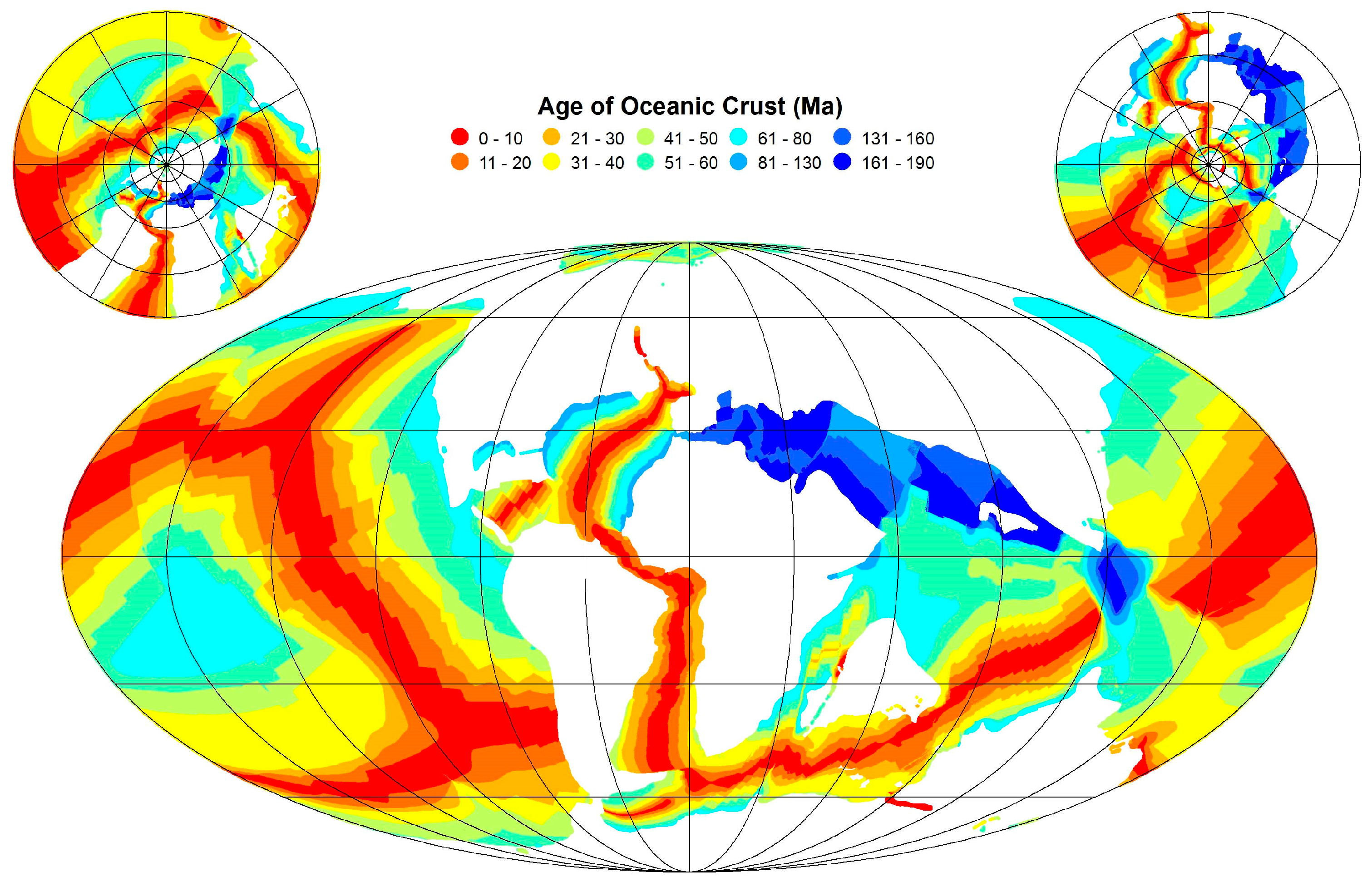
Ocean crust age: Müller [16] published global reconstructions of ocean crust age in 1 Myr intervals for the past 140 million years. For each reconstructed age in [16], ocean crust age, depth to basement, and bathymetry are given. This reconstructed bathymetry obtained as part of the dataset provided by Müller [16] is referred to hereafter as EB08 (EB: EarthByte). These data are in 0.1° × 0.1° resolution (3601 longitude × 1801 latitude points). For this project, (modern) crustal age reconstruction data are used (Figure 1).
Three geologic time scales that concern the age of the Cenomanian–Turonian (C–T) boundary are summarized in Table 1. The geologic time scale used by Müller et al. (2008) assigns a 36.9 m.y. duration from the top of C-Sequence chron C34 to the base of M-Sequence chron M0. The Cretaceous time scale in GTS2012 assigns a 42.66 m.y. duration and GTS2016 a 42.1 m.y. duration for the same interval, based on revised ages for the top of chron C34 and base of M0.
The C–T boundary age is now extremely well constrained at 93.9 Ma [48]. The duration of the interval from the C–T boundary to the top of C34 is estimated to be from 8.875 m.y. (GTS2012) to 8.5 m.y. (GTS2016), i.e., 23% to 24% of the duration of the C34 to M0 interval. This scales the C–T boundary age in the Müller GTS to between 92.375 Ma and 92.0 Ma. This differs slightly from the 93.5 Ma C–T boundary age of Gradstein [49], whose time scale was used to calibrate the digital age grid for the oceanic crust by Müller [31] and later used in EB08 [15].
Our study assumed a “traditional” age of 90 Ma for the C–T boundary for the ocean crustal component (construction of EB08). However, our reconstruction is actually between 2.375 m.y. and 2 m.y. younger than the C–T boundary age according to the Müller GTS (see Table 1), the latter presumably equivalent to the 93.9 Ma age of the C–T boundary assigned by GTS2012 and GTS2016.
Modern ocean sediment thickness: Modern ocean sediment thickness data from Divins [51] and Whittaker [52] are used. These data are derived from seismic profiling of the world’s ocean basins and other sources. The reported thicknesses are calculated using seismic velocity profiles that yield minimum thicknesses. Data values represent the distance between the seafloor and “acoustic basement”. The data are given in 5s × 5s resolution and have been regridded to 0.1° × 0.1° resolution values to match the EB08 grid [35].
ETOPO1: To reconstruct shelf-slope-rise structures, large igneous provinces and seamounts, modern topography and bathymetry from ETOPO1 [53] is used. The “Bedrock” version of ETOPO1 is utilized for this work, which is available in a 1s × 1s resolution (earthmodels.org), and regridded to 0.1° × 0.1° resolution [35] in order to match the EB08 grid. This version of ETOPO1 includes relief of Earth’s surface depicting the bedrock underneath the ice sheets. However, only the oceanic points in this dataset are used, so that there is no impact on the reconstructed bathymetry.
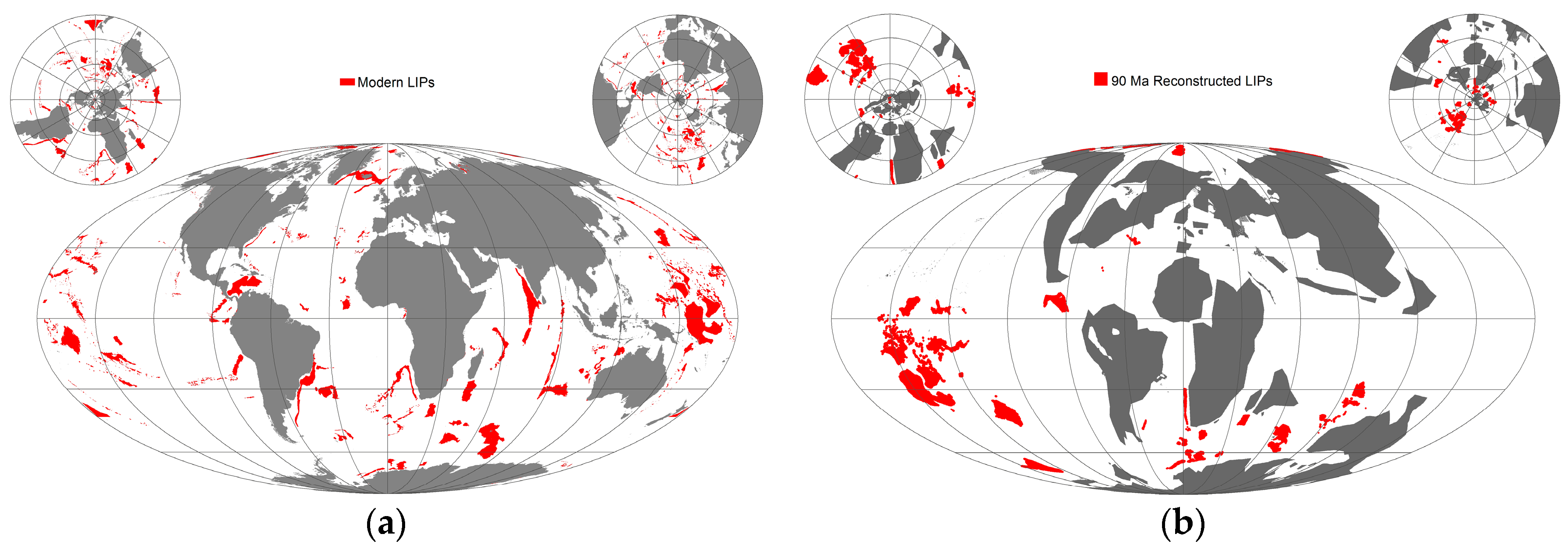
Large igneous provinces: In this reconstruction, the large igneous provinces (LIPs) dataset [54] is used. This dataset includes a geographic description of each LIP (Figure 2), plate identification number, and times of appearance and disappearance (in Ma). These LIPs are distinguished from mid-ocean ridge and subduction-related rocks based on petrology, geochemistry, geochronology, physical volcanology, and geophysical data. For this study only oceanic LIPs are considered. The modern distribution of the oceanic LIPs (Figure 2a) were rotated back to 94 Ma (Figure 2b).
Global Seamount Database: In this study, the seamounts from the Global Seamount Database [55] are used, which is based on satellite-derived vertical gravity gradient (VGG) data with globally 24,643 potential seamounts that are higher than or equal to 0.1 km, and located away from continental margins. The modern distributions of these seamounts (Figure 3a) were rotated back to 94 Ma (Figure 3b).
2.2. Methods
For this reconstruction, a standard plate cooling model for the oceanic lithosphere is combined with the age of the oceanic crust, global oceanic sediment thicknesses, plus generalized shelf-slope-rise structures calibrated at modern active and passive continental margins. As with the modern ocean basins, there are different types of crust: oceanic crust, submerged continental crust, and a transitional zone between the two (e.g., [35]). In this reconstruction, the regions underlain by oceanic crust to which an age has been assigned are termed “open ocean” regions. Here, a negative sign is assigned to signify depths below mean sea level (MSL).
The reconstruction of open ocean bathymetry starts with ocean crust age (Figure 1). This information is available only at locations where oceanic crust is preserved or has been reconstructed. The ocean depth-to-basement (Figure 4) is calculated based on a cooling plate with an average depth of −2639.8 m for the depth of mid-oceanic ridge [35].
The addition of sediment and an isostatic correction from sediment loading of the depth-to-basement oceanic crust (e.g., [56]) is critical to complete the bathymetric reconstruction of the open ocean region. A parameterized multilayer sediment cover, called “OES sediment thickness”, based on a third-degree polynomial fit between area corrected global sediment thickness data of modern oceans and marginal seas [51,52] and the age of the underlying oceanic crust [35], was isostatically added on top of the depth-to-basement. The sediment loading approach used here is similar to procedures used by Crough [57] and Sykes [58], was adopted using a multicomponent sediment layer with varying sediment densities calculated from a linear extrapolation of published sediment densities [35]. Once the sediment loading was added, the reconstruction of the open ocean regions was considered complete (Figure 5), and ready for merging with shelf-slope-rise structures, and adding LIPs, plateaus and seamounts, as will be described next.
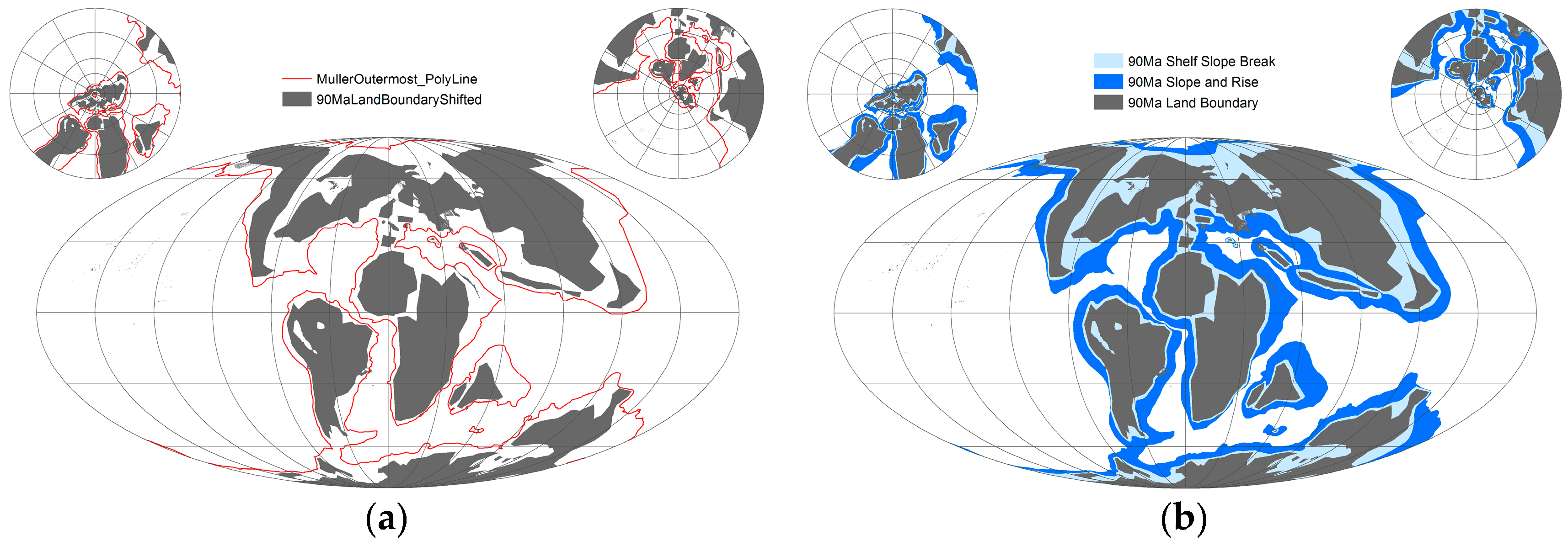
The parts of the ocean basins that occupy the transitional zone between oceanic crust and the emergent continental crust are termed here as “shelf-slope-rise” regions. These regions typically extend from the boundary of open ocean regions to the coastline. The three-parameter “shelf-slope-rise” model from Goswami [35], based on analysis of various modern shelf-slope-rise structures at active and passive margin regions from ETOPO1, along with their corresponding sediment thicknesses taken from [51], was used to reconstruct the C–T “shelf-slope-rise” regions, extending from the maximum extent ocean crust to the coastlines (Figure 6).
The paleo-shoreline model used in this reconstruction was obtained from the C–T paleo-DEM obtained from the PALEOMAP Project [41]. In this model, a zero meter coastline was extracted from the paleo-DEM to be used along with the EB08 ocean age grid map. When the extracted continental shorelines from the PALEOMAP Project reconstructions were incorporated into the EB08 CT age grid, there was a very small difference in the rotation of the continental South America block. This was manually adjusted to match with the EB08 grid.
The construction of the shelf-slope model is a combination of geographic information system and hand drawing activity. The process starts with drawing perpendicular lines to the paleo-coastline. Once the normal distance between the coastline and the shoreline has been defined, the nearest ocean crust is determined, and the shelf, slope and rise [35] dimensions are marked.
Accordingly, as detailed in [35] the C–T open-ocean regions (Figure 5) are then merged with C–T shelf-slope-rise regions (Figure 6). To accomplish this merging, map-based operations such as computing distances between locations were carried out using ArcGIS, and local calculations with interpolation were carried out in Matlab. The merged C–T base reconstructed bathymetry is shown in Figure 7.
This reconstructed C–T bathymetry was then updated with known oceanic LIPs and seamounts (Figure 2b and Figure 3b), for which GPlates (www.gplates.org) was used to rotate the modern distribution of the LIPs and seamounts back to C–T time. This updated reconstructed bathymetry was then smoothed and cleaned in Matlab using kriging interpolation. The final map of C–T reconstructed bathymetry is presented in Figure 8.
In sum, the final products are global maps of C–T depth-to-basement at 0.1° × 0.1° resolution (Figure 4), C–T paleobathymetry for the open oceans with an isostatically adjusted multicomponent sediment layer at 0.1° × 0.1° resolution (Figure 5), C–T paleobathymetry with reconstructed continental shelf-slope-rise structures (Figure 7) and a realistic combined C–T paleobathymetry with known LIPs and seamounts, continental shelf-slope-rise structures, and isostatically adjusted multicomponent sediment layer at 0.1° × 0.1° resolution (Figure 8).
3. Results
Here, the general nature of the C–T reconstructed bathymetry is discussed. One important point is that this bathymetric reconstruction was updated only with known LIPs and seamounts. As is clear from Figure 2b and Figure 3b, only certain areas in the central Pacific, Indian, proto-Caribbean and the North Atlantic Ocean therefore could be updated with seamounts and LIPs.
3.1. Reconstructed C–T Shelf-Slope-Rise Regions
The reconstructed C–T bathymetry (Figure 8) indicates that the global distribution of the continental blocks was more clustered than the modern world. North America and Eurasia were still connected, a young north Atlantic was spreading, and the central and southern Atlantic was in a juvenile state. In the south, Indian Ocean was also in its infancy while in between Indian peninsula and Eurasia was huge and mature Tethys Ocean. This unique paleogeography was quite different from the modern world and consequently influenced the C–T shelf-slope-rise regions.
Table 2 presents a comparison between the percentages of the global area for continents, oceans, continental shelf, slope and rise. Of the first order, during the C–T time, the area of the land was about 4% less of the global total area than the present world. Here, land refers to the part of the continental plate that is not submerged. Comparing with modern land areas, it is almost 14% less. All of the continental blocks were separated at this point of time, as the rifting of the supercontinent Pangea continued, though they were not far from each other. Accordingly, the ocean area was 4% larger in terms of total global area, and 5.66% greater the present-day world. These differences may be attributed to the growth in the size of the continents due to collisional tectonics [59].
Oceanic eustasy coupled with terrigenous sediment supply from newly separated continental interiors contributed to the development of mature shelf-slope-rise regions. As discussed in [35], typically the extent of these mature shelf-slope-rise regions extends beyond the maximum extent of ocean crust towards the shoreline. During C–T time, besides the major continental blocks including Africa, America, Eurasia, Antarctica, and India separating from the main Pangean aggregated supercontinent, many small-scale tectonic events took place that contributed to further expansion of shelf-slope-rise regions. For example, Madagascar separated from India, and the Kohistan-Ladakh Arc was rapidly approaching the northern boundary of the Indian peninsula [60]. In the northern Tethys between the North Atlantic and NW Tethys there were several smaller continental blocks. Surrounding both big and small continental blocks, development of shelf-slope rise structures was critical. The presence of an equatorial-tropical seaway connecting the Tethys to the Atlantic oceans, and the shallow but significantly wide Western Interior Seaway connecting the Gulf of Mexico to the Arctic Ocean, and a shallow African Seaway all added to the larger fraction of the shelf-slope-rise area during C–T time.
As summarized in Table 2, the total area occupied by all of the shelf-slope-rise regions was about 22.3% of the global area. Just shelf alone was 8.60% of the global area. Compared to modern combined shelf-slope-rise area, C–T shelf-slope-rise area was larger by more than 30%. The C–T shallow shelf was 8.60% of global area compared to 5.68% for the modern world. In other words, this was more than 60% of modern shelf area. Considering the continental slope and rise together the trend is not so similar, and was about 16% larger during C–T time. In sum, the most significant difference between modern and C–T oceans was in the area of the shelf region. Consequently, from a bathymetric point of view, this additional shallow shelf area and intermediate depth slope-rise area gave the C–T oceanic world a unique dimension.
3.2. Reconstructed C–T Open Ocean Region
Beyond the shelf-slope-rise region is the open ocean region. According to Table 2, the area of the C–T open ocean region is most comparable to that of the modern open ocean regions, only 2.61% less than today. The majority of the C–T open ocean region was part of the Pacific Ocean (Figure 1), extending around the newly rifted and separated continental landmasses. It was a giant young ocean basin with well-defined mid-oceanic ridge system creating new ocean floor. The North Atlantic had very limited area as open ocean. The South and Central Atlantic had negligible open ocean regions as these ocean basins had just started rifting South America from Africa. Also, the proto Caribbean Sea was rifting the South American block from North America. To the east, the other major ocean was the Tethys, which later would be completely subsumed between the Eurasian block and the fast-moving Indian block. The northern and northwestern part of the Tethys Ocean floor was the oldest among the global C–T ocean floors. Among all the other C–T oceans, the Tethys was unique as it did not have a well-developed, active ridge system. The Indian Ocean began to rift open between the Indian peninsula and Antarctica-Australia block. This long and linear rift extended to the eastern part of the Tethys. The Indian mid-oceanic ridge was separated from the Pacific ridge system by a smaller old oceanic block, which may have originally been part of eastern Tethys.
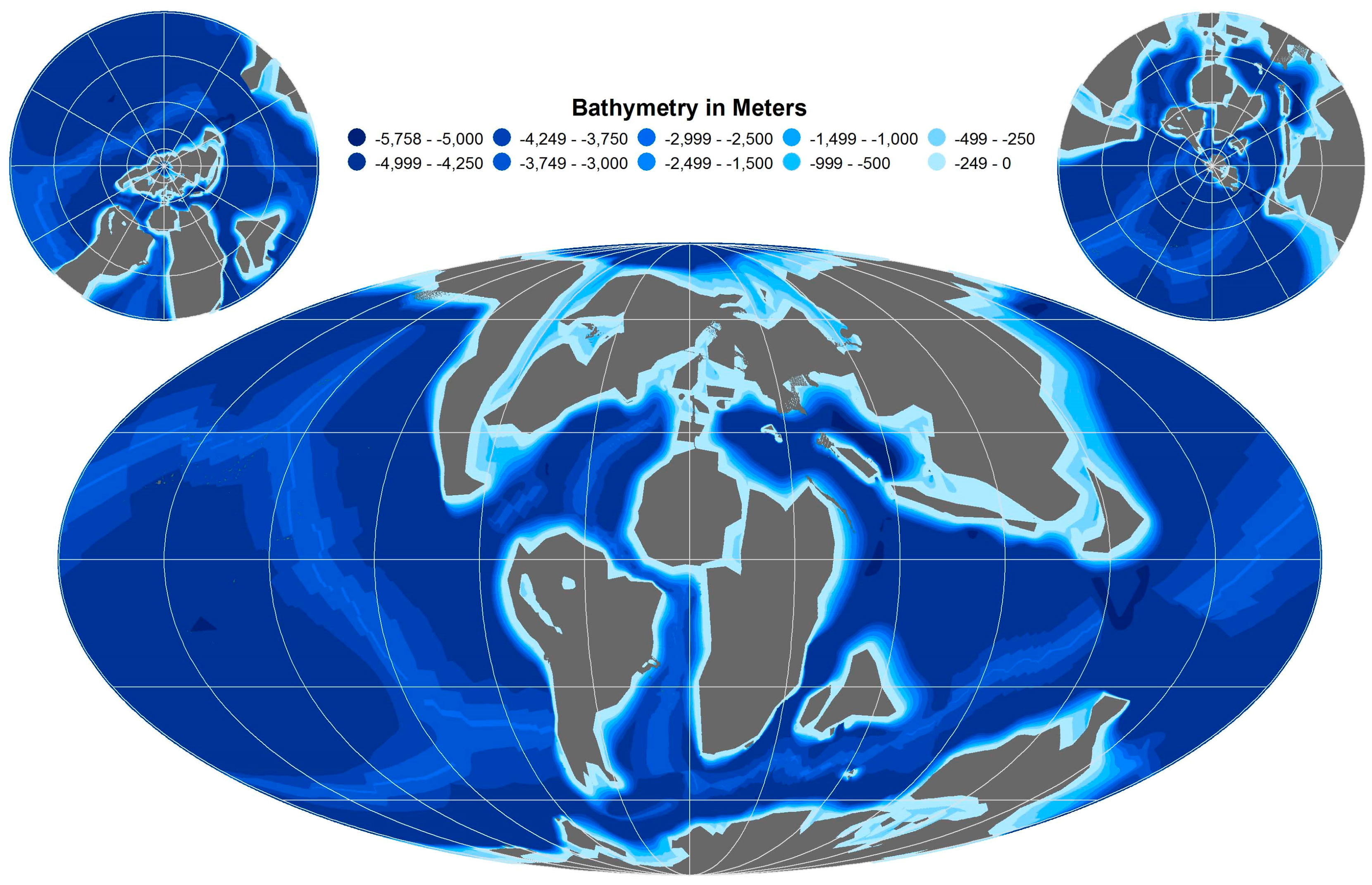
The maximum depth of the C–T open ocean region was about 5758 m, with a mean depth of 3262 m and median depth of 4080 m. C–T open oceans were shallower compared with modern open oceans. But looking at the median depth of the C–T open ocean was slightly deeper than that of the modern open oceans. In this regard, one of the final processing steps involved kriging interpolation to eliminate outlier calculation points. The total number of such points (19,285) was very small compared to the total number of points that define the entire C–T open ocean (4,498,703), i.e., less than 0.29%. Positive bathymetric values were changed to 0 using kriging type interpolation methods. Figure 9 shows the distribution of such points on top of the Interpolated 94 Ma reconstructed bathymetry (Figure 8).
Table 3 shows the statistics for modern and C–T ocean floor age, and the various steps of reconstructed C–T bathymetry in contrast to modern bathymetry (obtained from ETOPO1). The mean age of C–T ocean crust was about 40 million years (Myr) whereas the modern ocean crust has a mean age of about 63 Myr. Thus, on average, C–T oceanic crust was younger than the modern equivalent. The median ages corroborate the same view with C–T being about 36 Myr while the modern ocean is about 55 Myr. Looking at the mode value for C–T oceanic crust a drastic difference is revealed. While the age of modern oceanic crust has most common value of 0 Myr, for C–T oceanic crust it was 190 Myr. Thus C–T oceanic crust had overall older crustal age than the modern ocean. The overall statistics for the C–T reconstructed bathymetry are also provided in Table 3 and Supplementary Figure S3. The output of the plate model, listed as C–T depth-to-basement has maximum and minimum depths of 5555 m and 2663 m, respectively; the average depth is 4465 m. With loading from modeled sediment layers, these values change to 4920, 1385, and 4025 m, respectively. When the shelf-slope-rise wedge model is added to the open ocean reconstruction to obtain the C–T base bathymetry the signature changes to 5760 m, 677 m (above sea level) and 3305 m respectively for maximum, minimum and average depths (Supplementary Figure S4).
The minimum depth of 677 m above sea level is the result of outliers generated by the mathematical calculations. These outliers were later corrected using kriging type interpolation. The number of these outliers were very small compared to the scope of the entire dataset, (19,285 out of 4,498,703, which is less than 0.29%). The addition of oceanic LIPs and seamounts (both before and after interpolation) did not change the result of fixing the values programmatically for these 19,285 points. These erroneous points (Supplemental Figure S1) are mostly clustered, distributed in low to high latitudes of the Northern Hemisphere, and cover 0.031% of global C–T area (0.04% of global C–T ocean area).
Modern ocean bathymetric statistics derived from ETOPO1 are comparable to the C–T statistics. Although the modern ocean has much deeper trenches, the C–T ocean has a maximum depth of 5758 m, with an average depth of 3233 m, which is surprising similar to the modern (95.44%), which is 3388 m. The median depths of the modern and C–T oceans are also significantly similar, 3863 and 4005 m (103.7%), respectively. The difference may be attributed to the much older overall crustal age of the C–T ocean (see above). The most striking similarity is that the standard deviation of the OES C–T dataset is 100.88% of modern dataset. Another surprising similarity is in variance of these two datasets is within 2% range (Table 3).
4. Discussion
The reconstructed global C–T bathymetry presented here is the first of its kind based on the observations from modern ocean bathymetry. The main goal of OES is to reconstruct global paleobathymetry, provided age of the oceanic crust, onto which a generalized shelf-slope-rise structure model (based on present-day geometry) is anchored. The EB08 dataset was adopted for oceanic crustal ages. Along with the age of the oceanic crust for the last 140 Myr, EB08 also provides a version of depth-to-basement calculation and thereby a paleobathymetry (global in nature but without shelf-slope-rise) for each of the last 140 Myr in one Myr increments. The comparison of different statistical parameters between models are shown in Supplementary Figure S5.
Accordingly, the discussion starts with the comparison between EB08 (Supplementary Figure S1) and OES. The depth-to-basement reconstructions of OES and EB08 are similar in terms of minimum, mean, median, and mode depths. The difference is observed in the standard deviation, as the EB08 depth-to-basement has a maximum value which is positive. This is due to the fact that EB08 includes LIPs in the depth-to-basement whereas OES reconstruction does not. In Table 3, C–T OES final interpolated reconstructed bathymetry and its various components are compared with EB08, and SW07 bathymetries, which are very different. While OES bathymetry has a mean depth of 3233 meters, EB08 bathymetry has a mean depth of 4269 m. While compared to OES bathymetry trimmed to EB08 extent the mean value for OES bathymetry is 4070 meters. So overall, EB08 reconstructed bathymetry is on an average 200 m deeper in the open ocean regions. The OES full extent bathymetry is but much shallower than EB08 because of the shelf-slope-rise regions. The major difference in the EB08 bathymetry and the OES bathymetry EB08 extent is clear in variance, the measure of how far each value in the data set is from the mean. The variance for the OES bathymetry dataset (full bathymetry) is extraordinarily analogous to the variance of modern world bathymetry. The OES bathymetry dataset (EB08 extent), compared to EB08, has much smaller variance signifying gradual changes in bathymetry than that in EB08. This is confirmed by the modal and median values which shows that OES bathymetry has shallower median values as well as very shallow depths as the most common values. In EB08, the mode is very high at 5150 m as opposed to 6.5 m in OES. When compared to the OES bathymetry trimmed to EB08 extent, high modal value 4878 m (though much less than EB08, 5150 m) is observed. This exactly spells out the difference between the two bathymetry dataset and highlights the importance of reconstructing the shelf-slope-wedge. This has special significance especially for the C–T time, as for decades the paleoclimate community has argued for extensive shallow epicontinental seas [36,62,63,64,65,66,67,68,69,70,71,72,73,74,75,76] for example, to explain oceanic anoxic events. The OES C–T Ocean compared to Modern Ocean, has 4.75% more area (ocean area) less than 1000 m deep (maximum extent of combined euphotic and disphotic zone depth). For areas shallower than 500 m and 200 m, the OES C–T Ocean has 3.69% and 1.21% more compared to the Modern Ocean (Supplementary Table S1). The corresponding maps showing the extent of the reconstructed OES C–T ocean with these depths are shown in Supplementary Figure S6. These increased areas of shallower depths (compared to total ocean areas) are encouraging because OES reconstructed bathymetry at least in the case of C–T time, reconstructed larger areas of shallower depths in agreement with previously postulated arguments.
The difference between the depth-to-basement and final bathymetry also sheds some light regarding how much sediment was used in these bathymetric reconstructions, although caution is needed as direct measurement of sediment amount was not involved. Isostatic loading of sediment is complicated owing to density and thickness of sediment layers. The OES model shows a significant difference in the depth-to-basement to final bathymetric reconstruction (Table 3, OES Difference). Addition of sediment, modeled shelf-slope-rise structures and known seamounts and oceanic LIPs significantly change the final bathymetry with a much larger standard deviation. This is also seconded by the median values of the two models: OES median value is 48 m and EB08 median value is 205 m. This implies that the changes in depth-to-basement to final bathymetry in the OES reconstruction does not involve many abrupt changes (or less abrupt changes) in depth, and rather, follows a natural gradient, which may be more realistic. A high median value, on the other hand, implies that in EB08, there are unexpected abrupt variations in the bathymetric values. The most common value (mode) in the OES difference dataset is 675 m, while the mean is 385 m. In EB08, these values are considerably lower, 490 m and 250 m, respectively.
When compared with the modern ocean bathymetry the OES C–T reconstructed bathymetry reflects interesting similarity. Though it is created using the very different ocean crustal age (see Table 3) than the modern one, the average and median depth, mode, standard deviation and the variance of the modern ocean and C–T ocean are highly comparable (Table 3). Surprisingly, these two datasets (modern and OES C–T) have less agreement with the EB08 reconstructed bathymetry.
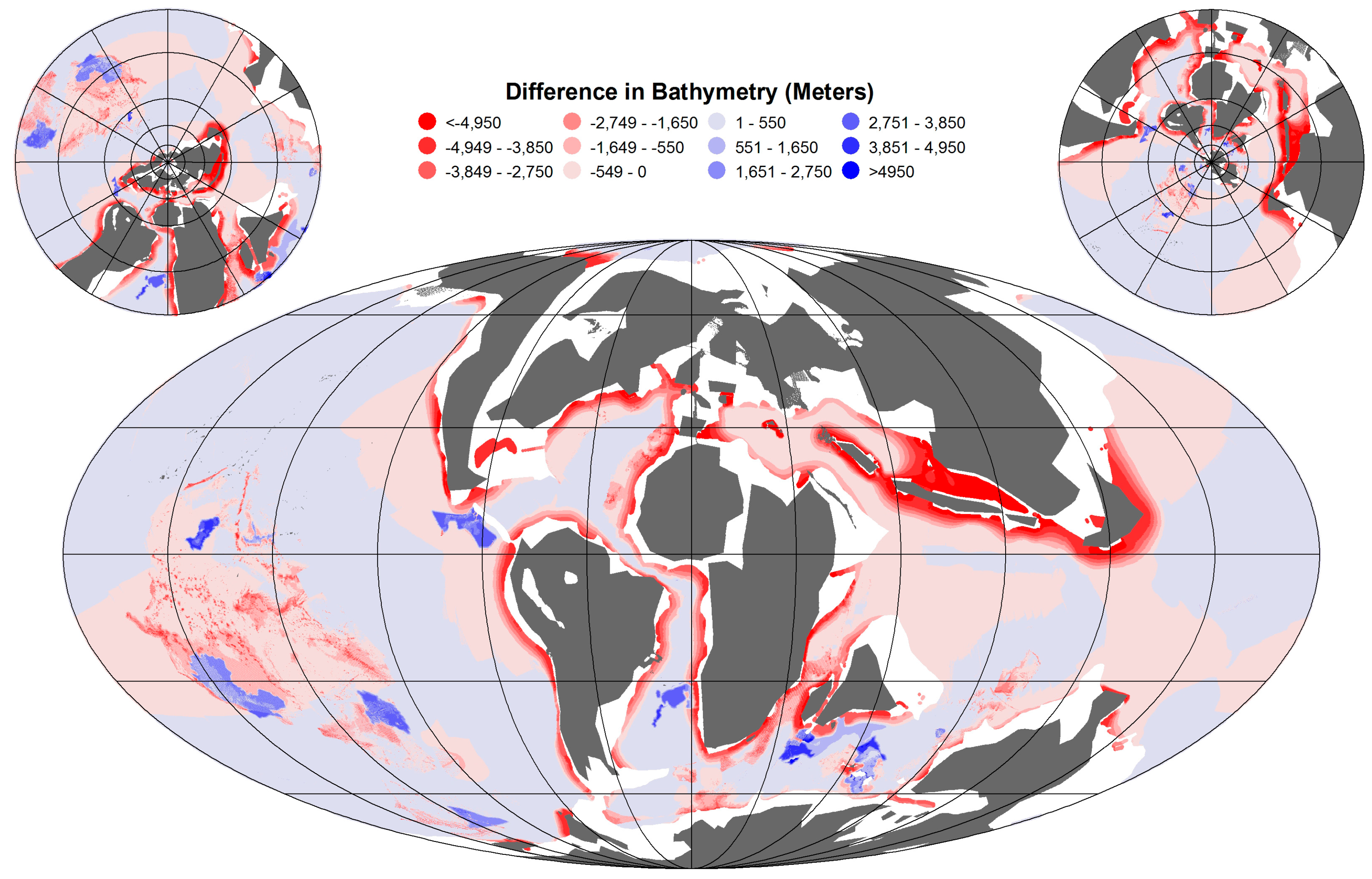
Other than statistical comparison, a difference map between the EB08 and OES C–T reconstructions is given in Figure 10. The red tone signifies that EB08 reconstruction is deeper while blue tone signifies the OES reconstruction is deeper. Statistics for this difference map are provided in Table 3, but also computed EB08 extent (mainly open oceans regions) as EB08 does not have shelf-slope-rise structures. Both maximum and minimum values for the difference plots are very large. The maximum value of 5640 m are in the regions where there are underwater LIPs. In EB08, these areas have positive values signifying they are above the water and sometimes even up to 2000+ m. In the OES reconstruction, all known LIPs are added, but they all have an average depth of at least 1500 m. Similarly, the high minimum number is near the outer (oldest) edge of the oceanic crust, where in the OES reconstruction, the shelf-slope-rise model is added to estimate natural coastal landforms. Much of the open ocean regions in the two models are in agreement and their mean difference is 190 m with a high standard deviation.
Another interesting comparison can be made with the C–T bathymetric model of Sewall [2] (SW07). The SW07 model is available in a 64 × 128 grid size, and here is resized to 1801 × 3601 (Supplementary Figure S2) in order to compare with the OES model. The SW07 model also contains topography; only values less than or equal to zero were considered for comparison (Figure 11). The statistical comparison between the OES and SW07 models indicates some fascinating similarity. The minimum, mean and median depths are within 10% of each other. The modal depth, however, is very different, in OES bathymetry being very shallow (6.5 m), while that in SW07 is very deep (5040 m). The standard deviations of these two models are 10% (OES) and 20% (SW07). In the SW07-OES difference map (Figure 11), regions with positive values indicate deeper depths in OES. Most of the disagreements are in the continental shelf-slope-rise regions and may be attributed to the shelf-slope-rise structure of the OES model. There are also some differences in the depth of mid-oceanic ridges: in OES, the mid-oceanic ridges are much shallower than in SW07. Both models include a larger and more open North Atlantic Ocean; extensive Cretaceous interior seaways in North and South America, North Africa, and Eastern Europe, and a narrowly open South Atlantic Ocean.
In addition to the Cretaceous paleobathymetric reconstruction presented here, there are other important related developments that are very encouraging. Hochmuth and Gohl [33] are working on improving geodynamic and paleoceanographic aspects related to ocean crustal age with a high-resolution plate kinematic model. The alternative seafloor age grid for the South Atlantic Ocean based on a recent high-resolution plate kinematic model [43] is of particular interest due to its connection to the Cretaceous Normal Superchron. Enhanced studies like this will open the door for better understanding of long-offset fracture zones, currently mostly overlooked in paleobathymetric reconstructions.
The C–T transition occurred during the wettest, hottest climates of the Cretaceous greenhouse with assists from greenhouse gases emitted to the atmosphere by unusually large mid-ocean ridge systems and mantle plume magmatism [77]. The opening of the critical N-S Equatorial Atlantic Seaway coincided with a change from an “eddy ocean” to a “thermohaline ocean” [78]. Evidence for this change is provided by North Atlantic nannofossils which evolved from homogeneous Cenomanian distributions with cosmopolitan ranges to heterogeneous Turonian distributions with restricted ranges [40].
The Earth’s equator-to-pole temperature gradient is a fundamental climatological property related to equator-to-pole heat transport efficiency, ocean circulation, hydrological cycling and atmospheric chemistry [79]. The meriodional thermal gradient may have been at its lowest in the Cretaceous during the C–T transition. Unfortunately, Cretaceous paleoclimate modeling with GCMs has consistently underestimated the warm polar temperatures that are indicated by fossil and geochemical data (e.g., [74,80,81]).
Realistic paleobathymetries are among the improvements that can be tested in GCM paleoclimate simulations. The goal of this project has been to address this by producing a more realistic ocean floor with continental shelf-slope-rise, underwater ridges, trenches, seamounts, LIPs and a corresponding ocean bottom roughness. In particular, seafloor roughness and topography exert critical controls on vertical ocean mixing and circulation [82,83]. Will our paleobathymetry provide clues for understanding the eddy-dominated Cenomanian ocean? What would cause ocean reorganization in the Turonian—development of a less rough seafloor due to more rapid seafloor spreading [42,83].
5. Conclusions
The ongoing goal of OESbathy reconstruction is to provide a means for reconstructing realistic paleobathymetries for geologic times that can be tied directly to ocean crustal age. The innovation of OESbathy is the generalized shelf-slope-rise model to provide bathymetric interpolation across the transitional zone between open ocean and coastlines; this model is described in detail for the test case modern day OESbathy 1.0 reconstruction [35]. Here OESbathy has been extended to Cenomanian–Turonian (C–T) boundary time (94 Ma), and updated with known oceanic LIPs and seamounts. The main results are as follows:
- Parameterized shelf-slope-rise structures result in a much shallower mean ocean depth than other available C–T bathymetry reconstructions.
- C–T ocean crust was on average 40.29 million years old whereas modern ocean crust has a mean age of 63.39 million years.
- The OES C–T ocean has an average depth of 3262 m, while the modern ocean average depth is 3388 m. Despite that the OES C–T Ocean is about 125 m shallower, the overall ocean bathymetric pattern matches with the modern bathymetric values as both have similar standard deviations (within 1%) despite significantly different maximum and average depths.
- Seafloor roughness is provided from mid-ocean ridges, and oceanic LIPS and sea mounts rotated to their C–T positions (using known features).
The following improvements are being planned: (1) The OES sediment model will be validated and corrected using data from DSDP/ODP/IODP. (2) The OES shelf-slope-rise model will be revisited with a more detailed parameterization of modern active and passive margins. (3) We are working on the reconstruction of ocean bottom surface fractures, especially those near the mid-ocean ridge areas, and experimenting with statistical models to simulate seafloor roughness. (4) An OES reconstruction of Paleocene–Eocene Thermal Maximum (55 Myr) paleobathymetry is now underway.
Supplementary Materials
The following are available online at www.mdpi.com/2076-3263/8/1/21/s1; Figure S1: EB08 C–T bathymetry; Figure S2: SW07 [2] C–T bathymetry (from the total land ocean topography bathymetry, only the values zero or below have been plotted here); Figure S3: Comparative statistics of modern and C–T ages of the ocean crust (in Ma). The minimum is not shown as both have zero as minimum ocean crust age; Figure S4: Comparison of the three models. OES: Interpolated OES CT Bathymetry, OES*: Interpolated OES CT Bathymetry trimmed to EB08 extent, EB08: EB08 CT Bathymetry, and SW07: SW07 CT Bathymetry; Figure S5: Comparison between different of OES C–T bathymetry development. Step 1: OES Depth-to-Basement. Step 2: OES Depth-to-Basement isostatically loaded with multilayer sediments. Step 3: OES C–T Base Bathymetry with shelf-slope-rise. Step 4: OES Bathymetry with known LIPs and Seamounts, and Step 5: OES Interpolated Bathymetry; Figure S6: OES C-T Ocean showing (A) areas of 200, 500 and 1000 meters depths; (B) area of 200 meters depth; (C) area of 500 meters depth; and (D) area of 1000 meters depth. Table S1: Comparison of shallow ocean areas between Modern and C–T oceans.
Acknowledgments
A significant portion of this work was supported by Frontiers in Earth System Dynamics grant EAR-1135382 from the National Science Foundation. Also, the authors are thankful to C. R. Scotese for sharing the SW07 datasets used in this study for comparison. The authors highly appreciate the invitation from the MDPI publication group for the invitation to this special marine geomorphometry issue.
Author Contributions
Data for the open ocean reconstruction and sediment wedge model were acquired and analyzed by Arghya Goswami. The reconstruction algorithm was developed by Arghya Goswami under the guidance of Ananad Gnanadesikan) and Linda Hinnov. Taylor Young acquired the data related to LIPs and seamounts, and after preparation and analysis, updated the C–T paleobathymetry. Arghya Ggoswami did the main writing while Linda Hhinnov did the editing.
Conflicts of Interest
The authors declare no conflict of interest.
References
- Markwick, P.J.; Valdes, P.J. Palaeo-digital elevation models for use as boundary conditions in coupled ocean–atmosphere GCM experiments: A Maastrichtian (late Cretaceous) example. Palaeogeogr. Palaeoclimatol. Palaeoecol. 2004, 213, 37–63. [Google Scholar] [CrossRef]
- Sewall, J.O.; Van De Wal, R.S.W.; Van Der Zwan, K.; Van Oosterhout, C.; Dijkstra, H.A.; Scotese, C.R. Climate model boundary conditions for four Cretaceous time slices. Clim. Past 2007, 3, 647–657. [Google Scholar] [CrossRef]
- Lunt, D.J.; Huber, M.; Anagnostou, E.; Baatsen, M.L.J.; Caballero, R.; DeConto, R.; Dijkstra, H.A.; Donnadieu, Y.; Evans, D.; Feng, R.; et al. The DeepMIP contribution to PMIP4: Experimental design for model simulations of the EECO, PETM, and pre-PETM (version 1.0). Geosci. Model Dev. 2017, 10, 889–901. [Google Scholar] [CrossRef]
- Barron, E.J.; Washington, W.M. The role of geographic variables in explaining paleoclimates: Results from Cretaceous climate model sensitivity studies. J. Geophys. Res. Atmos. 1984, 89, 1267–1279. [Google Scholar] [CrossRef]
- Barron, E.J. Explanations of the Tertiary global cooling trend. Palaeogeogr. Palaeoclimatol. Palaeoecol. 1985, 50, 45–61. [Google Scholar] [CrossRef]
- Chandler, M.A.; Rind, D.; Ruedy, R. Pangaean climate during the Early Jurassic: GCM simulations and the sedimentary record of paleoclimate. Geol. Soc. Am. Bull. 1992, 104, 543–559. [Google Scholar] [CrossRef]
- Barron, E.J.; Fawcett, P.J.; Pollard, D.; Thompson, S. Model simulations of Cretaceous climates: The role of geography and carbon dioxide. Philos. Trans. R. Soc. Lond. B Biol. Sci. 1993, 341, 307–316. [Google Scholar] [CrossRef]
- Barron, E.J.; Moore, G.T. Climate Model Application in Paleoenvironmental Analysis; Society for Sedimentary Geology (SEPM): Tulsa, OK, USA, 1994. [Google Scholar]
- Price, G.D.; Sellwood, B.W.; Valdes, P.J. Sedimentological evaluation of general circulation model simulations for the “greenhouse” Earth: Cretaceous and Jurassic case studies. Sediment. Geol. 1995, 100, 159–180. [Google Scholar] [CrossRef]
- Poulsen, C.J.; Barron, E.J.; Peterson, W.H.; Wilson, P.A. A reinterpretation of Mid-Cretaceous shallow marine temperatures through model-data comparison. Paleoceanography 1999, 14, 679–697. [Google Scholar] [CrossRef]
- Upchurch, G.R.; Otto-Bliesner, B.L.; Scotese, C.R. Terrestrial Vegetation and Its Effects on Climate during the Latest Cretaceous; Special Papers; Geological Society of America: Boulder, CO, USA, 1999; pp. 407–426. [Google Scholar]
- DeConto, R.M.; Brady, E.C.; Bergengren, J.; Hay, W.W. Late Cretaceous climate, vegetation, and ocean interactions. In Warm Climates in Earth History; Cambridge University Press: Cambridge, UK, 2000; pp. 275–296. [Google Scholar]
- Poulsen, C.J.; Gendaszek, A.S.; Jacob, R.L. Did the rifting of the Atlantic Ocean cause the Cretaceous thermal maximum? Geology 2003, 31, 115–118. [Google Scholar] [CrossRef]
- Hay, W.W.; Floegel, S. New thoughts about the Cretaceous climate and oceans. Earth-Sci. Rev. 2012, 115, 262–272. [Google Scholar] [CrossRef]
- Müller, R.D.; Sdrolias, M.; Gaina, C.; Roest, W.R. Age, spreading rates, and spreading asymmetry of the world’s ocean crust. Geochem. Geophys. Geosyst. 2008, 9, 1–19. [Google Scholar] [CrossRef]
- Müller, R.D.; Sdrolias, M.; Gaina, C.; Steinberger, B.; Heine, C. Long-term sea-level fluctuations driven by ocean basin dynamics. Science 2008, 319, 1357–1362. [Google Scholar] [CrossRef] [PubMed]
- Wells, M.R.; Allison, P.A.; Piggott, M.D.; Hampson, G.J.; Pain, C.C.; Gorman, G.J. Tidal modeling of an ancient tide-dominated seaway, part 1: Model validation and application to global early Cretaceous (Aptian) tides. J. Sediment. Res. 2010, 80, 393–410. [Google Scholar] [CrossRef]
- Bice, K.L.; Barron, E.J.; Peterson, W.H. Reconstruction of realistic early Eocene paleobathymetry and ocean GCM sensitivity to specified basin configuration. Oxf. Monogr. Geol. Geophys. 1998, 39, 227–250. [Google Scholar]
- Sclater, J.G.; Abbott, D.; Thiede, J. Paleobathymetry and sediments of the Indian Ocean. In Indian Ocean Geology and Biostratigraphy; Wiley: New York, NY, USA, 1977; pp. 25–59. [Google Scholar]
- Sclater, J.G.; Hellinger, S.; Tapscott, C. The paleobathymetry of the Atlantic Ocean from the Jurassic to the present. J. Geol. 1977, 85, 509–552. [Google Scholar] [CrossRef]
- Herkat, M. Application of correspondence analysis to palaeobathymetric reconstruction of Cenomanian and Turonian (Cretaceous) rocks of Eastern Algeria. Palaeogeogr. Palaeoclimatol. Palaeoecol. 2007, 254, 583–605. [Google Scholar] [CrossRef]
- Sageman, B.B.; Arthur, M.A. Early Turonian paleogeographic/paleobathymetric map, western interior, US. In Mesozoic Systems of the Rocky Mountain Region; Society for Sedimentary Geology (SEPM): Tulsa, OK, USA, 1994. [Google Scholar]
- Kyrkjebø, R.; Kjennerud, T.; Gillmore, G.K.; Faleide, J.I.; Gabrielsen, R.H. Cretaceous-Tertiary palaeo-bathymetry in the northern North Sea; integration of palaeo-water depth estimates obtained by structural restoration and micropalaeontological analysis. Nor. Pet. Soc. Spec. Publ. 2001, 10, 321–345. [Google Scholar]
- Butt, A. Micropaleontological bathymetry of the Cretaceous of Western Morocco. Palaeogeogr. Palaeoclimatol. Palaeoecol. 1982, 37, 235245265–242261275. [Google Scholar] [CrossRef]
- Topper, R.P.M.; Trabucho Alexandre, J.; Tuenter, E.; Meijer, P.T. A regional ocean circulation model for the mid-Cretaceous North Atlantic Basin: Implications for black shale formation. Clim. Past 2011, 7, 277–297. [Google Scholar] [CrossRef] [Green Version]
- Krupitsky, A.; Kamenkovich, V.M.; Naik, N.; Cane, M.A. A linear equivalent barotropic model of the Antarctic Circumpolar Current with realistic coastlines and bottom topography. J. Phys. Oceanogr. 1996, 26, 1803–1824. [Google Scholar] [CrossRef]
- Wright, J.D.; Miller, K.G. Control of North Atlantic deep water circulation by the Greenland-Scotland Ridge. Paleoceanography 1996, 11, 157–170. [Google Scholar] [CrossRef]
- Simmons, H.L.; Jayne, S.R.; Laurent, L.C.S.; Weaver, A.J. Tidally driven mixing in a numerical model of the ocean general circulation. Ocean Model. 2004, 6, 245–263. [Google Scholar] [CrossRef]
- Sijp, W.P.; England, M.H. Role of the Drake Passage in controlling the stability of the ocean’s thermohaline circulation. J. Clim. 2005, 18, 1957–1966. [Google Scholar] [CrossRef]
- Parsons, B.; Sclater, J.G. An analysis of the variation of ocean floor bathymetry and heat flow with age. J. Geophys. Res. 1977, 82, 803–827. [Google Scholar] [CrossRef]
- Müller, R.D.; Roest, W.R.; Royer, J.-Y.; Gahagan, L.M.; Sclater, J.G. Digital isochrons of the world’s ocean floor. J. Geophys. Res. Solid Earth 1997, 102, 3211–3214. [Google Scholar] [CrossRef]
- Xu, X.; Lithgow-Bertelloni, C.; Conrad, C.P. Global reconstructions of Cenozoic seafloor ages: Implications for bathymetry and sea level. Earth Planet. Sci. Lett. 2006, 243, 552–564. [Google Scholar] [CrossRef]
- Hochmuth, K.; Gohl, K. Paleobathymetry of the Southern Ocean and its role in paleoclimate and paleo-ice sheet variations–A call for a sequence of community paleobathymetric grids. In Proceedings of the SCAR Open Science Conference, Kuala Lumpur, Malaysia, 10–20 August 2016. [Google Scholar]
- Hayes, D.E.; Zhang, C.; Weissel, R.A. Modeling paleobathymetry in the Southern Ocean. Eos Trans. Am. Geophys. Union 2009, 90, 165–166. [Google Scholar] [CrossRef]
- Goswami, A.; Olson, P.L.; Hinnov, L.A.; Gnanadesikan, A. OESbathy version 1.0: A method for reconstructing ocean bathymetry with generalized continental shelf-slope-rise structures. Geosci. Model Dev. 2015, 8, 2735–2748. [Google Scholar] [CrossRef]
- Jenkyns, H.C. Geochemistry of oceanic anoxic events. Geochem. Geophys. Geosyst. 2010, 11. [Google Scholar] [CrossRef]
- Klemme, H.D.; Ulmishek, G.F. Effective petroleum source rocks of the world: Stratigraphic distribution and controlling depositional factors. AAPG Bull. 1991, 75, 1809–1851. [Google Scholar]
- Jarvis, I.; Lignum, J.S.; Gröcke, D.R.; Jenkyns, H.C.; Pearce, M.A. Black shale deposition, atmospheric CO2 drawdown, and cooling during the Cenomanian-Turonian Oceanic Anoxic Event. Paleoceanography 2011, 26. [Google Scholar] [CrossRef]
- Bryan, S.E.; Ferrari, L. Large igneous provinces and silicic large igneous provinces: Progress in our understanding over the last 25 years. Geol. Soc. Am. Bull. 2013, 125, 1053–1078. [Google Scholar] [CrossRef] [Green Version]
- Linnert, C.; Mutterlose, J.; Herrle, J.O. Late Cretaceous (Cenomanian–Maastrichtian) calcareous nannofossils from Goban Spur (DSDP Sites 549, 551): Implications for the palaeoceanography of the proto North Atlantic. Palaeogeogr. Palaeoclimatol. Palaeoecol. 2011, 299, 507–528. [Google Scholar] [CrossRef]
- Scotese, C.R. Atlas of Late Cretaceous Paleogeographic Maps, PALEOMAP Atlas for ArcGIS, Volume 2, The Cretaceous, Maps 16–22, Mollweide Projection, PALEOMAP Project, Evanston, IL; Technical Report for PALEOMAP Project: Evanston, IL, USA, 2014. [Google Scholar]
- Granot, R.; Dyment, J. The Cretaceous opening of the South Atlantic Ocean. Earth Planet. Sci. Lett. 2015, 414, 156–163. [Google Scholar] [CrossRef]
- Pérez-Díaz, L.; Eagles, G. A new high-resolution seafloor age grid for the South Atlantic. Geochem. Geophys. Geosyst. 2017, 18, 457–470. [Google Scholar] [CrossRef]
- Channell, J.E.T.; Horvath, F. The African/Adriatic promontory as a palaeogeographical premise for Alpine orogeny and plate movements in the Carpatho-Balkan region. Tectonophysics 1976, 35, 71–101. [Google Scholar] [CrossRef]
- Rosenbaum, G.; Lister, G.S.; Duboz, C. Relative motions of Africa, Iberia and Europe during Alpine orogeny. Tectonophysics 2002, 359, 117–129. [Google Scholar] [CrossRef]
- Basilone, L.; Perri, F.; Sulli, A.; Critelli, S. Paleoclimate and extensional tectonics of short-lived lacustrine environments. Lower Cretaceous of the Panormide Southern Tethyan carbonate platform (NW Sicily). Mar. Pet. Geol. 2017, 88, 428–439. [Google Scholar] [CrossRef]
- Basilone, L.; Sulli, A. Basin analysis in the Southern Tethyan margin: Facies sequences, stratal pattern and subsidence history highlight extension-to-inversion processes in the Cretaceous Panormide carbonate platform (NW Sicily). Sediment. Geol. 2018, 363, 235–251. [Google Scholar] [CrossRef]
- Ogg, J.G.; Ogg, G.; Gradstein, F.M. A Concise Geologic Time Scale: 2016; Elsevier: Amsterdam, The Netherlands, 2016. [Google Scholar]
- Gradstein, F.M.; Agterberg, F.P.; Ogg, J.G.; Hardenbol, J.; Veen, P.; Thierry, J.; Huang, Z. A Mesozoic time scale. J. Geophys. Res. Solid Earth 1994, 99, 24051–24074. [Google Scholar] [CrossRef]
- Divins, D.L. Total Sediment Thickness of the World’s Oceans and Marginal Seas; NOAA National Geophysical Data Center: Boulder, CO, USA, 2003.
- Whittaker, J.M.; Goncharov, A.; Williams, S.E.; Müller, R.D.; Leitchenkov, G. Global sediment thickness data set updated for the Australian-Antarctic Southern Ocean. Geochem. Geophys. Geosyst. 2013, 14, 3297–3305. [Google Scholar] [CrossRef]
- Ogg, J.G.; Hinnov, L.A.; Huang, C. Cretaceous. In The Geologic Time Scale; Chapter 27; Elsevier: Amsterdam, The Netherlands, 2012; pp. 793–853. [Google Scholar]
- Amante, C.; Eakins, B.W. ETOPO1 1 Arc-Minute Global Relief Model: Procedures, Data Sources and Analysis; Marine Geology and Geophysics Division: Boulder, CO, USA, 2009. [Google Scholar]
- Coffin, M.F.; Duncan, R.A.; Eldholm, O.; Fitton, J.G.; Frey, F.A.; Larsen, H.C.; Mahoney, J.J.; Saunders, A.D.; Schlich, R.; Wallace, P.J. Large igneous provinces and scientific ocean drilling: Status quo and a look ahead. Oceanography 2006, 19, 150–160. [Google Scholar] [CrossRef]
- Kim, S.-S.; Wessel, P. New global seamount census from altimetry-derived gravity data. Geophys. J. Int. 2011, 186, 615–631. [Google Scholar] [CrossRef]
- Celerier, B. Paleobathymetry and geodynamic models for subsidence. Palaios 1988, 3, 454–463. [Google Scholar] [CrossRef]
- Crough, S.T. The correction for sediment loading on the seafloor. J. Geophys. Res. Solid Earth 1983, 88, 6449–6454. [Google Scholar] [CrossRef]
- Sykes, T.J. A correction for sediment load upon the ocean floor: Uniform versus varying sediment density estimations—Implications for isostatic correction. Mar. Geol. 1996, 133, 35–49. [Google Scholar] [CrossRef]
- Niu, Y.; Zhao, Z.; Zhu, D.-C.; Mo, X. Continental collision zones are primary sites for net continental crust growth—A testable hypothesis. Earth-Sci. Rev. 2013, 127, 96–110. [Google Scholar] [CrossRef]
- Encyclopedia Britannica | Britannica.com. Available online: https://www.britannica.com/ (accessed on 12 December 2017).
- Chatterjee, S.; Goswami, A.; Scotese, C.R. The longest voyage: Tectonic, magmatic, and paleoclimatic evolution of the Indian plate during its northward flight from Gondwana to Asia. Gondwana Res. 2013, 23, 238–267. [Google Scholar] [CrossRef]
- Schlanger, S.O.; Jenkyns, H.C. Cretaceous oceanic anoxic events: Causes and consequences. Geol. Mijnb. 1976, 55, 179–184. [Google Scholar]
- Schlanger, S.O.; Arthur, M.A.; Jenkyns, H.C.; Scholle, P.A. The Cenomanian-Turonian Oceanic Anoxic Event, I. Stratigraphy and distribution of organic carbon-rich beds and the marine δ13C excursion. Geol. Soc. Lond. Spec. Publ. 1987, 26, 371–399. [Google Scholar] [CrossRef]
- Arthur, M.A.; Schlanger, S.T.; Jenkyns, H.C. The Cenomanian-Turonian Oceanic Anoxic Event, II. Palaeoceanographic controls on organic-matter production and preservation. Geol. Soc. Lond. Spec. Publ. 1987, 26, 401–420. [Google Scholar] [CrossRef]
- Thurow, J.; Brumsack, H.-J.; Rullkötter, J.; Littke, R.; Meyers, P. The Cenomanian/Turonian boundary event in the Indian Ocean: A key to understand the global picture. In Synthesis of Results from Scientific Drilling in the Indian Ocean; Geophysical Monograph Series; Wiley: New York, NY, USA, 1992; Volume 70, pp. 253–273. [Google Scholar]
- Damsté, J.S.S.; Köster, J. A euxinic southern North Atlantic Ocean during the Cenomanian/Turonian oceanic anoxic event. Earth Planet. Sci. Lett. 1998, 158, 165–173. [Google Scholar] [CrossRef]
- Tsikos, H.; Jenkyns, H.C.; Walsworth-Bell, B.; Petrizzo, M.R.; Forster, A.; Kolonic, S.; Erba, E.; Silva, I.P.; Baas, M.; Wagner, T. Carbon-isotope stratigraphy recorded by the Cenomanian–Turonian Oceanic Anoxic Event: Correlation and implications based on three key localities. J. Geol. Soc. 2004, 161, 711–719. [Google Scholar] [CrossRef]
- Parente, M.; Frijia, G.; Di Lucia, M. Carbon-isotope stratigraphy of Cenomanian–Turonian platform carbonates from the southern Apennines (Italy): A chemostratigraphic approach to the problem of correlation between shallow-water and deep-water successions. J. Geol. Soc. 2007, 164, 609–620. [Google Scholar] [CrossRef]
- Parente, M.; Frijia, G.; Di Lucia, M.; Jenkyns, H.C.; Woodfine, R.G.; Baroncini, F. Stepwise extinction of larger foraminifers at the Cenomanian-Turonian boundary: A shallow-water perspective on nutrient fluctuations during Oceanic Anoxic Event 2 (Bonarelli Event). Geology 2008, 36, 715–718. [Google Scholar] [CrossRef]
- Gebhardt, H.; Friedrich, O.; Schenk, B.; Fox, L.; Hart, M.; Wagreich, M. Paleoceanographic changes at the northern Tethyan margin during the Cenomanian–Turonian Oceanic Anoxic Event (OAE-2). Mar. Micropaleontol. 2010, 77, 25–45. [Google Scholar] [CrossRef]
- Owens, J.D.; Lyons, T.W.; Li, X.; Macleod, K.G.; Gordon, G.; Kuypers, M.M.M.; Anbar, A.; Kuhnt, W.; Severmann, S. Iron isotope and trace metal records of iron cycling in the proto-North Atlantic during the Cenomanian-Turonian oceanic anoxic event (OAE-2). Paleoceanography 2012, 27. [Google Scholar] [CrossRef]
- Zheng, X.-Y.; Jenkyns, H.C.; Gale, A.S.; Ward, D.J.; Henderson, G.M. Changing ocean circulation and hydrothermal inputs during Ocean Anoxic Event 2 (Cenomanian–Turonian): Evidence from Nd-isotopes in the European shelf sea. Earth Planet. Sci. Lett. 2013, 375, 338–348. [Google Scholar] [CrossRef]
- Zhou, X.; Jenkyns, H.C.; Owens, J.D.; Junium, C.K.; Zheng, X.-Y.; Sageman, B.B.; Hardisty, D.S.; Lyons, T.W.; Ridgwell, A.; Lu, Z. Upper ocean oxygenation dynamics from I/Ca ratios during the Cenomanian-Turonian OAE2. Paleoceanography 2015, 30, 510–526. [Google Scholar] [CrossRef]
- Friedrich, O.; Erbacher, J.; Mutterlose, J. Paleoenvironmental changes across the Cenomanian/Turonian boundary event (oceanic anoxic event 2) as indicated by benthic foraminifera from the Demerara Rise (ODP Leg 207). Rev. Micropaléontol. 2006, 49, 121–139. [Google Scholar] [CrossRef]
- Gertsch, B.; Keller, G.; Adatte, T.; Berner, Z.; Kassab, A.S.; Tantawy, A.A.A.; El-Sabbagh, A.M.; Stueben, D. Cenomanian–Turonian transition in a shallow water sequence of the Sinai. Egypt. Int. J. Earth Sci. 2008, 99, 165–182. [Google Scholar] [CrossRef]
- Gertsch, B.; Adatte, T.; Keller, G.; Tantawy, A.A.A.M.; Berner, Z.; Mort, H.P.; Fleitmann, D. Middle and late Cenomanian oceanic anoxic events in shallow and deeper shelf environments of western Morocco. Sedimentology 2010, 57, 1430–1462. [Google Scholar] [CrossRef]
- Hay, W.W. Toward understanding Cretaceous climate—An updated review. Sci. China Earth Sci. 2017, 60, 5–19. [Google Scholar] [CrossRef]
- Hay, W.W. Evolving ideas about the Cretaceous climate and ocean circulation. Cretac. Res. 2008, 29, 725–753. [Google Scholar] [CrossRef]
- Cronin, T.M. Paleoclimates: Understanding Climate Change Past and Present; Columbia University Press: New York, NY, USA, 2009. [Google Scholar]
- DeConto, R.M.; Hay, W.W.; Thompson, S.L.; Bergengren, J. Late Cretaceous Climate and Vegetation Interactions: Cold Continental Interior Paradox; Special Papers; Geological Society of America: Boulder, CO, USA, 1999; pp. 391–406. [Google Scholar]
- Sellwood, B.W.; Valdes, P.J. Mesozoic climates: General circulation models and the rock record. Sediment. Geol. 2006, 190, 269–287. [Google Scholar] [CrossRef]
- Jayne, S.R.; St Laurent, L.C.; Gille, S.T. Connections between ocean bottom topography and Earth’s climate. Oceanography 2004, 17, 65–74. [Google Scholar] [CrossRef]
- Sandwell, D.T.; Smith, W.H.; Gille, S.; Kappel, E.; Jayne, S.; Soofi, K.; Coakley, B.; Géli, L. Bathymetry from space: Rationale and requirements for a new, high-resolution altimetric mission. C. R. Geosci. 2006, 338, 1049–1062. [Google Scholar] [CrossRef]
Figure 1.
Age of the ocean crust for Cenomanian–Turonian (C–T) time (94 Ma), derived from Müller et al. [15].
Figure 1.
Age of the ocean crust for Cenomanian–Turonian (C–T) time (94 Ma), derived from Müller et al. [15].

Figure 2.
Distribution of Large Igneous Provinces (LIPs) in the ocean basins. (a) Modern; (b) 94 Ma.
Figure 2.
Distribution of Large Igneous Provinces (LIPs) in the ocean basins. (a) Modern; (b) 94 Ma.

Figure 3.
Distribution of seamounts in the ocean basins. (a) Modern; (b) 94 Ma.

Figure 4.
Depth-to-basement calculated from the age of oceanic crust at 94 Ma.

Figure 5.
Depth-to-basement, with isostatically adjusted, multicomponent sediment layer at 94 Ma.

Figure 6.
The extent of different 94 Ma ocean boundaries. (a) The maximum extent of the ocean crust in the ocean basins; (b) the extent of 94 Ma land, shelf, slope, and rise.
Figure 6.
The extent of different 94 Ma ocean boundaries. (a) The maximum extent of the ocean crust in the ocean basins; (b) the extent of 94 Ma land, shelf, slope, and rise.

Figure 7.
The 94 Ma reconstructed base bathymetry with isostatically adjusted, multicomponent sediment layer and shelf-slope-rise structure.
Figure 7.
The 94 Ma reconstructed base bathymetry with isostatically adjusted, multicomponent sediment layer and shelf-slope-rise structure.

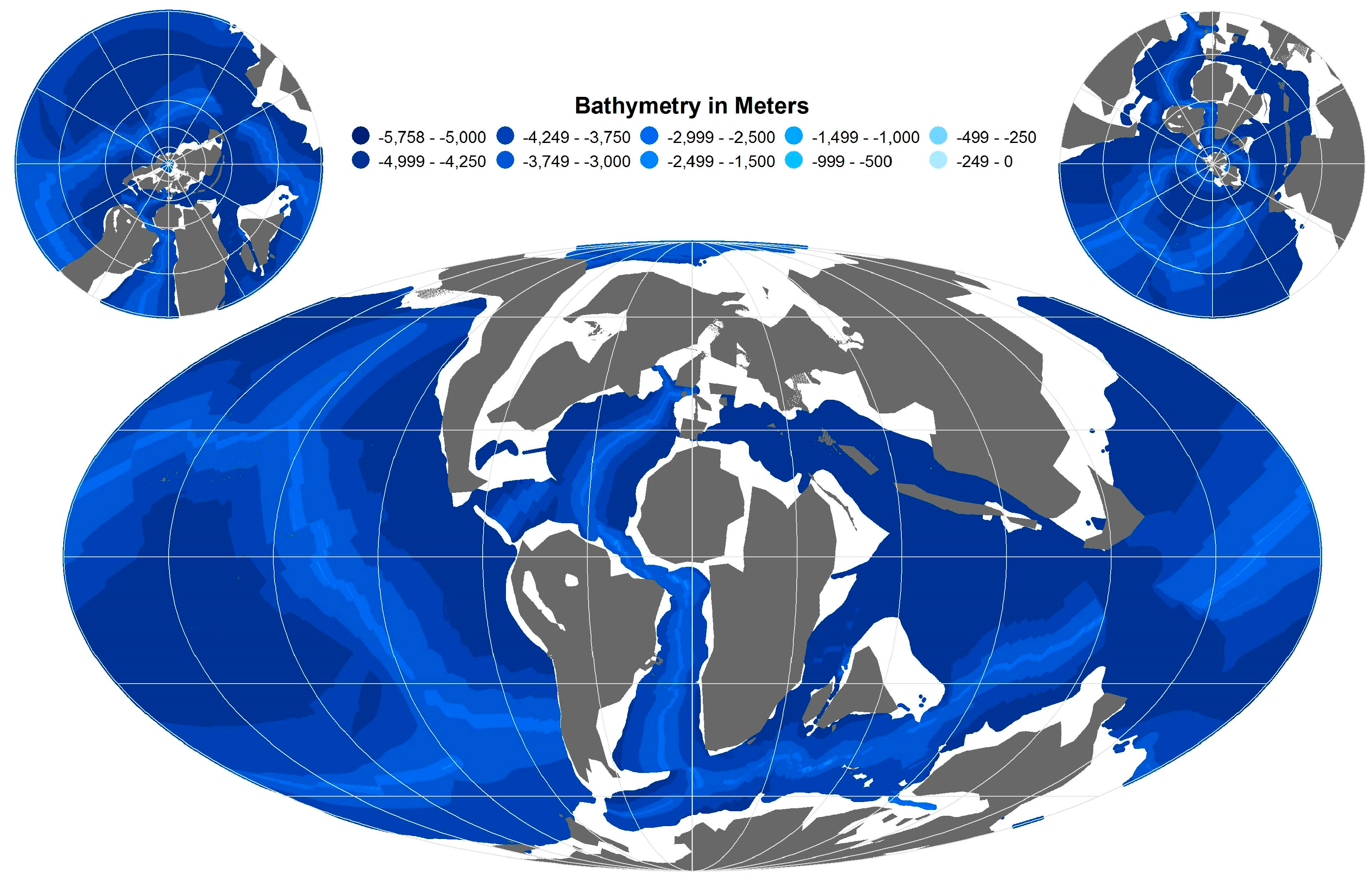
Figure 8.
Interpolated 94 Ma reconstructed bathymetry with isostatically adjusted, multicomponent sediment layer, continental shelf-slope-rise structures, and known LIPs and seamounts.
Figure 8.
Interpolated 94 Ma reconstructed bathymetry with isostatically adjusted, multicomponent sediment layer, continental shelf-slope-rise structures, and known LIPs and seamounts.

Figure 9.
Distribution of the interpolated points (in red) on top of the interpolated 94 Ma reconstructed bathymetry with isostatically adjusted, multicomponent sediment layer, continental shelf-slope-rise structures, and known LIPs and seamounts.
Figure 9.
Distribution of the interpolated points (in red) on top of the interpolated 94 Ma reconstructed bathymetry with isostatically adjusted, multicomponent sediment layer, continental shelf-slope-rise structures, and known LIPs and seamounts.

Figure 10.
Difference map between the EB08 and OES C–T reconstructions.

Figure 11.
Difference map between the SW07 and OES C–T reconstructions.


Table 1.
Geologic time scales, durations and ages of key boundaries. GTS2012 = The Geologic Time Scale for the Cretaceous Period [50]; GTS2016 = Concise Geologic Time Scale 2016 [48]; Müller GTS according to [15].
| GTS2012 | GTS2016 | Müller GTS | |
|---|---|---|---|
| Top C34 age | 83.64 Ma | 84.2 Ma | 83.5 Ma |
| Base M0 age | 126.3 Ma | 126.3 Ma | 120.4 Ma |
| Top C34 to base M0 duration | 42.66 m.y. | 42.1 m.y. | 36.9 m.y. |
| Top C34 to C–T boundary duration | 8.875 m.y. | 8.5 m.y. | 8.875 a m.y. or 8.5 b m.y. |
| C–T boundary age | 93.9 Ma | 93.9 Ma | 92.375 a Ma or 92.0 b Ma |
a Based on GTS2012 C34 to C–T boundary duration as 24% of the top C34 to base M0 duration. b Based on GTS2016 C34 to C–T boundary duration as 23% of the top C34 to base M0 duration.
Table 2.
Comparison of area between modern and C–T oceans.
| Modern World 1 | C–T World 2 | C–T/Modern | |
|---|---|---|---|
| Continents | 29.00% | 24.98% | −13.86% |
| Ocean | 71.00% | 75.02% | 5.66% |
| Continental shelf * | 5.68% | 8.60% | 51.47% |
| Continental slope and rise * | 11.72% | 13.70% | 16.93% |
| Combined shelf, slope and rise * | 17.40% | 22.31% | 28.20% |
| Open Ocean | 53.60% | 52.71% | −1.66% |
1 Data for modern world is taken from Encyclopedia of Britannica [61]; 2 Data for C–T world are according to this project; * Percent of total global area.
Table 3.
Comparative statistics of Open Earth Systems (OES), Modern and EB08 bathymetries.
| Variable | Max | Min | Mean | Mean % 9 | Median | Median % 9 | Mode | Std.Dev. | Std.Dev. % 9 | Variance | Variance % 9 |
|---|---|---|---|---|---|---|---|---|---|---|---|
| C–T OC1 Age 2 | 190.00 | 0.00 | 40.29 | 63.56% | 36.20 | 65.94% | 190.00 | 32.51 | 72.66% | 1057.17 | 52.81% |
| Modern OC1 Age 2 | 280.00 | 0.00 | 63.39 | 100.00% | 54.90 | 100.00% | 0.00 | 44.74 | 100.00% | 2001.77 | 100.00% |
| OES D2B 3 | −2662.69 | −5554.11 | −4464.67 | 131.79% | −4592.02 | 118.87% | −5554.11 | 604.00 | 34.69% | 364,819.64 | 12.03% |
| OES D2B3 + Sediment | −1385.96 | −4920.04 | −4024.87 | 118.81% | −4084.91 | 105.74% | −4671.99 | 527.11 | 30.27% | 277,844.40 | 9.17% |
| OES Base4 Bathymetry | 677.31 | −5758.30 | −3303.11 | 97.51% | −4128.30 | 106.87% | −6.52 | 1769.18 | 101.61% | 3,129,987.14 | 103.25% |
| OES Bathymetry 5 | 5087.88 | −5758.30 | −3229.23 | 95.32% | −4005.90 | 103.70% | −6.52 | 1764.88 | 101.36% | 3,114,784.82 | 102.75% |
| OES Difference 6 | 2283.91 | −5551.14 | −385.27 | − | −48.74 | − | −676.01 | 1018.68 | - | 1,037,718.60 | - |
| OES Interpolated Bathymetry | 0.00 | −5758.30 | −3233.20 | 95.44% | −4005.90 | 103.70% | −6.52 | 1756.50 | 100.88% | 3,085,309.63 | 101.77% |
| Modern Ocean Bathymetry 7 | −1.00 | −10,714.00 | −3387.63 | 100.00% | −3863.00 | 100.00% | −1.00 | 1741.13 | 100.00% | 3,031,539.27 | 100.00% |
| OES Interpolated EB08 Extent 8 | 0.00 | −5753.00 | −4070.70 | 120.16% | −4394.60 | 113.76% | −4878.10 | 995.00 | 57.15% | 990,018.77 | 32.66% |
| EB08 D2B 3 | 2290.43 | −5638.43 | −4520.08 | 133.43% | −4724.14 | 122.29% | −5638.43 | 803.68 | 46.16% | 645,909.44 | 21.31% |
| EB08 Bathymetry | 2402.45 | −5266.97 | −4269.14 | 126.02% | −4423.02 | 114.50% | −5150.16 | 753.15 | 43.26% | 567,234.14 | 18.71% |
| EB08 Difference 6 | −96.22 | −733.19 | −250.94 | − | −204.79 | − | −488.27 | 140.55 | - | 19,753.06 | - |
| SW07 C–T Ocean | 0.00 | −5755.90 | −3442.90 | 101.63% | −4508.39 | 116.71% | −5040.00 | 1970.61 | 113.18% | 3,883,318.54 | 128.10% |
1 OC = Ocean Crust; 2 Age in million annum (Ma). All other numbers are in meters; 3 D2B = Depth-to-basement; 4 Base = with sediment and shelf-slope-rise structure; 5 This maximum value and correlated positive values represent some points that become positive when different equations are applied. The number of such points with positive values (19,285) are very small compared to the total number of points in the entire ocean basin (4,498,703), approximately 0.29%. The calculated positive bathymetric values of these points were changed to 0 using kriging type interpolation methods; 6 difference = (depth-to-basement—final bathymetry); 7 Data source ETOPO1; 8 OES bathymetry trimmed to EB08 extent; 9 With respect to modern value.
© 2018 by the authors. Licensee MDPI, Basel, Switzerland. This article is an open access article distributed under the terms and conditions of the Creative Commons Attribution (CC BY) license (http://creativecommons.org/licenses/by/4.0/).
Share and Cite
MDPI and ACS Style
Goswami, A.; Hinnov, L.; Gnanadesikan, A.; Young, T. Realistic Paleobathymetry of the Cenomanian–Turonian (94 Ma) Boundary Global Ocean. Geosciences 2018, 8, 21. https://doi.org/10.3390/geosciences8010021
AMA Style
Goswami A, Hinnov L, Gnanadesikan A, Young T. Realistic Paleobathymetry of the Cenomanian–Turonian (94 Ma) Boundary Global Ocean. Geosciences. 2018; 8(1):21. https://doi.org/10.3390/geosciences8010021
Chicago/Turabian StyleGoswami, Arghya, Linda Hinnov, Anand Gnanadesikan, and Taylor Young. 2018. "Realistic Paleobathymetry of the Cenomanian–Turonian (94 Ma) Boundary Global Ocean" Geosciences 8, no. 1: 21. https://doi.org/10.3390/geosciences8010021
Note that from the first issue of 2016, this journal uses article numbers instead of page numbers. See further details here.