Probabilistic Substrate Classification with Multispectral Acoustic Backscatter: A Comparison of Discriminative and Generative Models


1
School of Earth & Sustainability, Northern Arizona University, Flagstaff, AZ 86011, USA
2
U.S. Geological Survey, Southwest Biological Science Center, Grand Canyon Monitoring & Research Center, Flagstaff, AZ 86001, USA
*
Author to whom correspondence should be addressed.
Geosciences 2018, 8(11), 395; https://doi.org/10.3390/geosciences8110395
Submission received: 5 October 2018
/
Revised: 22 October 2018
/
Accepted: 25 October 2018
/
Published: 30 October 2018
(This article belongs to the Special Issue Geological Seafloor Mapping)
Abstract
:We propose a probabilistic graphical model for discriminative substrate characterization, to support geological and biological habitat mapping in aquatic environments. The model, called a fully-connected conditional random field (CRF), is demonstrated using multispectral and monospectral acoustic backscatter from heterogeneous seafloors in Patricia Bay, British Columbia, and Bedford Basin, Nova Scotia. Unlike previously proposed discriminative algorithms, the CRF model considers both the relative backscatter magnitudes of different substrates and their relative proximities. The model therefore combines the statistical flexibility of a machine learning algorithm with an inherently spatial treatment of the substrate. The CRF model predicts substrates such that nearby locations with similar backscattering characteristics are likely to be in the same substrate class. The degree of allowable proximity and backscatter similarity are controlled by parameters that are learned from the data. CRF model results were evaluated against a popular generative model known as a Gaussian Mixture model (GMM) that doesn’t include spatial dependencies, only covariance between substrate backscattering response over different frequencies. Both models are used in conjunction with sparse bed observations/samples in a supervised classification. A detailed accuracy assessment, including a leave-one-out cross-validation analysis, was performed using both models. Using multispectral backscatter, the GMM model trained on 50% of the bed observations resulted in a 75% and 89% average accuracies in Patricia Bay and Bedford Basin, respectively. The same metrics for the CRF model were 78% and 95%. Further, the CRF model resulted in a 91% mean cross-validation accuracy across four substrate classes at Patricia Bay, and a 99.5% mean accuracy across three substrate classes at Bedford Basin, which suggest that the CRF model generalizes extremely well to new data. This analysis also showed that the CRF model was much less sensitive to the specific number and locations of bed observations than the generative model, owing to its ability to incorporate spatial autocorrelation in substrates. The CRF therefore may prove to be a powerful ‘spatially aware’ alternative to other discriminative classifiers.
1. Introduction
High resolution bathymetry and acoustic backscatter can be gathered in a cost-effective manner over large areas in aquatic systems with multibeam sonar. Automated substrate classification for benthic habitat and geologic mapping is a growing area of research [1,2,3] due to the efficiency with which dense information on both terrain and substrates may be collected with a single instrument, driven by a pressing need for accurate substrate maps for the purposes of marine spatial planning and management, design of marine protected areas, fisheries resource management, maritime archeology, minerals exploration, and scientific research in the fields of submarine geology and benthic ecology [4,5]. Similar needs in freshwater environments are driving increasing use of multibeam backscatter in rivers and lakes [6,7]. Recently, the appropriate collection and analysis of backscatter [8,9], including studies into the uncertainty [10] and repeatability [11] of backscatter measurements have made substrate acoustics a more accessible field for ecologists and geologists. The quantitative analysis of substrate topography has been reviewed by [12]. General overviews of substrate classification using multibeam acoustic backscatter are provided by [2,13].
Existing approaches to benthic substrate characterization using data collected by multibeam echosounders can be categorized as unsupervised, which determine the type and number of substrates from the data itself, or supervised (or ‘task-specific’) that estimate substrates based on some independent information about the distribution of sediments, such as physical samples or benthic photographs. Many unsupervised approaches employ analytical models that capture the physics of substrate-sound interactions [14,15] and are especially suitable for relatively simple clastic substrates at relatively low acoustic frequencies [6]. Supervised methods are more commonly used for heterogeneous substrates with a large biogenic component [4,16], especially at relatively high frequency (several hundred kilohertz) [17]. Supervised approaches typically require a set of training samples to find the relationship between relatively sparse ground-truth bed observations and features derived from multibeam data, to quantitatively describe the associated substrate [2]. Extrapolating this relationship to broad scales from limited observations requires robust spatial modeling. To that end, machine learning has proved a popular approach based on single frequency (monospectral) multibeam backscatter [4,18,19,20], for two principal reasons. First, the outputs are readily amenable to probabilistic interpretation, whereas quantification of spatially distributed uncertainty is more difficult to achieve using unsupervised approaches. Second, technological advances in collecting images of the bed using cabled and autonomous video systems [21] have been commensurate with advances in global positioning systems and inertial navigation, sonar hardware and automated substrate classification algorithms.
The goal of all probabilistic models for substrate classification is to find , that is, the conditional probability distribution of a single discrete label given a vector of features assigned to grid node , where can take any value from a pre-defined set, , numeric labels each corresponding to an observed discrete substrate substrate type. Feature vector may in practice be any combination of the primary data streams from multibeam echosounders (bathymetry and backscatter) or derived bathymetric products such as roughness, slope, aspect, etc [4,18] or derived backscatter metrics [22]. One way to formalize the problem is as a function approximation. We assume for some unknown function f. The goal of a machine learning algorithm is to estimate f given a labeled training data set, and then to make predictions using (the symbol denotes an estimate). To handle ambiguity, the most probable substrate type is found by solving, where C is a vector of possible substrate classes,
where
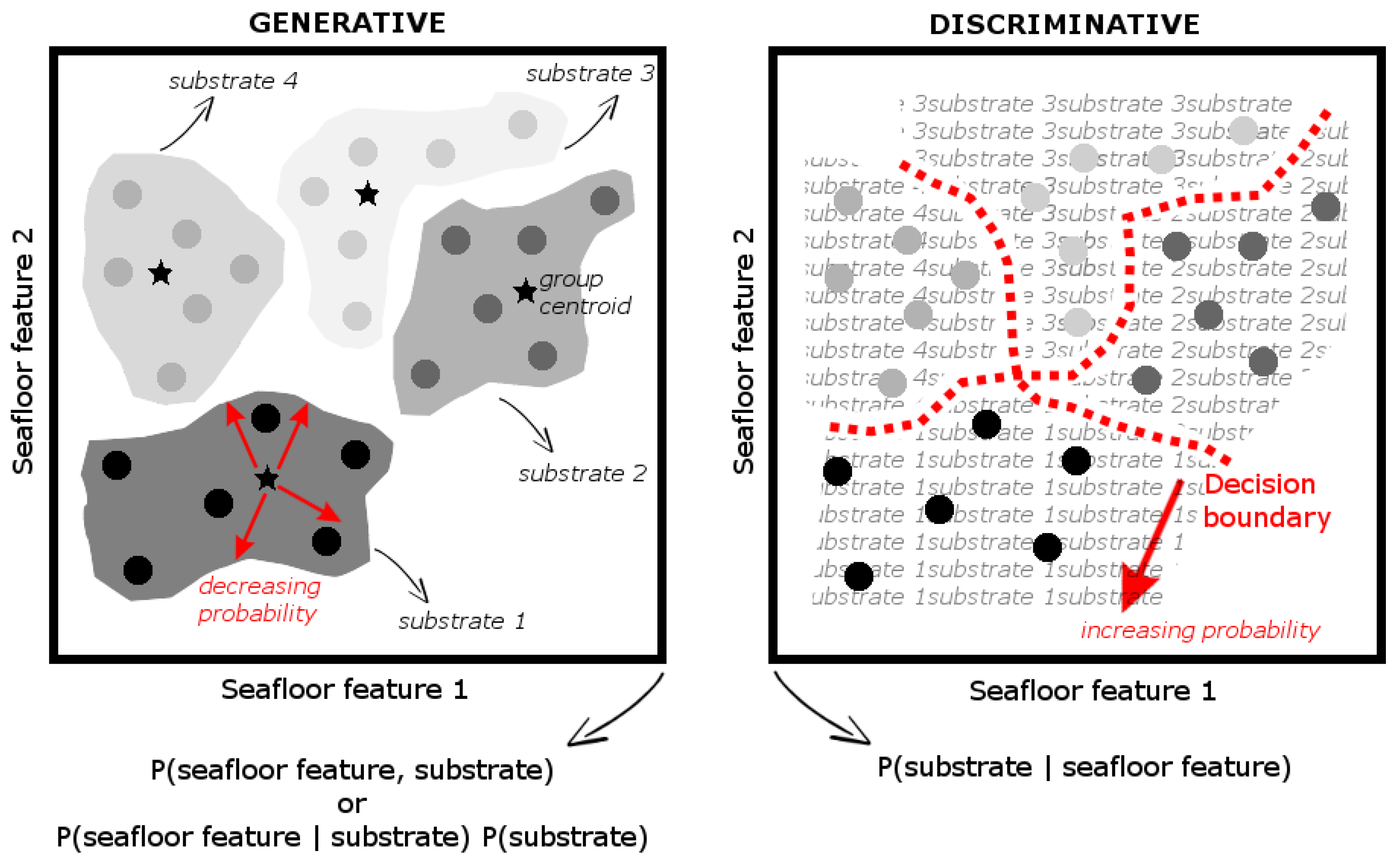
is the softmax function [23], in which denotes the inner product of and weight w and is the output of the model over K possible outcomes. One might break the classification problem down into two stages: The inference stage in which the training data (substrate features, x, and their substrate labels, y) are used to learn a model for , and the subsequent decision stage where we use these posterior probabilities to assign optimal labels. An alternative is to solve both the inference and decision stages simultaneously, by learning a discriminant function from the input data that maps inputs x directly into labels y. The difference between these two approaches is the difference between a generative [7,24] and a discriminative probabilistic model (Figure 1). A generative model estimates the probability distributions of individual substrate labels (classes) to then generate estimates of their posterior probabilities. With a discriminative model, instead of first modeling the joint distribution of and y together, , a conditional distribution of y given , is modeled directly, without attempting to model underlying (or ‘generating’) probability distributions. This bypasses the need to capture the distributions over , to model the correlations between them, and therefore to specify an underlying prior model that describes . Any chosen set of features may have complicated dependencies, and the relationships among , and between and y, might significantly change when applied to the next data set, the next location, the next time, the next spatial scale, etc. Discriminative approaches, including neural networks [25], support vector machines [18], decision trees [26], and random forests [27], have therefore been popular.
With the recent development of multispectral multibeam technology [28,29] it is now possible to examine the backscattering response of a set of substrates across multiple frequencies. With multispectral backscatter, a discriminative approach has much more information with which to draw its decision boundaries. However, until it is understood how substrates respond to multiple frequencies, we require a substrate model that does not rely on a statistical assumption of independence, which says that the substrate features do not depend on and affect each other. To that end, we describe a discriminative substrate classification algorithm that relaxes the independence assumption, for use with either mono- or multispectral backscatter, that may be applied in a supervised (y drawn from direct observations of the bed) framework. We evaluate the skill of the proposed classification method using multispectral backscatter data at two sites, comparing the classification results with those from a more standard generative machine learning algorithm, namely a Gaussian Mixture Model [6,7,24].
2. Methods
2.1. Discriminative Probabilistic Substrate Classification
2.1.1. Graphical Models
Graphical models are an efficient way to describe complex, high-dimensional distributions. Suppose we have a simple seafloor everywhere consisting of either sand or gravel, and also suppose we also have three extracted seafloor features called feature 1, feature 2, and feature 3. These features could be any relevant metric extracted from backscatter, bathymetry or other sources of available information such as hydrodynamic maps. Let’s further suppose each of our features may be valued 1 through 100. Overall, therefore, our probability space has 2 (sand or no sand) × 2 (gravel or no gravel) × 100 × 100 × 100 = 4 million values, corresponding to the possible assignments of the five variables. Our task is to evaluate the likelihood of each. Computing a joint probability distribution over this space allows us to ask questions such as how likely the substrate is sand given minimal values of all three features. The probability expression for this case encodes our beliefs about this particular situation, and would be
However, specifying a joint probability distribution over four million possible values could be a substantial computational task and, in reality, the seafloor typically consists of many more classes, and it may be possible to extract many more features that have many more possible values. Graphical models are an efficient way to describe such complex, high-dimensional distributions. The nodes in the graph correspond to our variables (substrates and features) and the edges between them correspond to the probabilistic interactions between them. The goal is to infer the structure of the graph, which tells us the set of independencies that hold for the distribution [30]. For example, our ‘target’ distribution P in Equation (3) may satisfy the conditional independence (feature 1 ⊥ feature 2 | gravel, sand) where ⊥ denotes ‘independent from’, which asserts that
The above says that, if we are interested in the distribution over feature 1, and we know whether the substrate is sand or gravel, feature 2 is no longer informative. However, this doesn’t imply that feature 2 is independent of feature 1, only that all the information we may obtain from feature 1 on the chances of feature 2 we already obtain by knowing whether the substrate is sand or gravel. The other advantage of the graphical model is that rather than encoding the probability of each of the 4 million values in our example, instead it facilitates breaking up the problem into smaller factors, each over a much smaller space of possibilities. The overall distribution is found as the product of these factors. For example, suppose that the probability of the event “feature 1=50, no sand, gravel, feature 2 = 100, feature 3 = 0” is found by multiplying five numbers: , , , , and . This representation is significantly more compact, requiring far fewer parameters than the original four million. The graph structure defines the factorization of P as a set of factors and the variables they encompass, called the ‘scope’ [30].
2.1.2. Conditional Random Field
A conditional random field (CRF) is an undirected graphical model that we use here to probabilistically predict substrate labels based on weak supervision, which in the present case is discrete label annotations of substrate types in discrete locations. Seafloor (backscatter) features and their associated labels y are mapped to graphs, whereby each node is connected by an edge to its neighbors according to a connectivity rule. Linking each node of the graph created from to every other node enables modeling of the long-range spatial connections within the data by considering both proximal and distal pairs of grid nodes, resulting in pixel (fine) scale labeling at boundaries and transitions between different label classes.
Conditional Random Fields (CRFs) [31] have been used extensively for task-specific predictions where estimates of labels for sparse regions of the data are used in conjunction with the underlying features, to draw decision boundaries for each label, resulting in a label per feature [32,33]. The primary advantage of CRFs for substrate classification is the relaxation of the independence assumption [31], which says that the substrate features do not depend on each other. Especially for multispectral backscatter, this is not always the case and it could lead to serious inaccuracies.
A CRF is parameterized the same as a Gibbs distribution, but is normalized differently. We start with an unnormalized measure of the joint distribution
where , are factors and where are a set of vectors of backscatter at each location i that are termed the ‘scope’ of their associated [30] (see previous subsection). In order to model the conditional distribution , a normalization constant (called a partition function), Z, is required that is a function of [30]:
Then the the probability of a substrate labeling y given the multibeam-derived data is
We model as a Gibbs energy function, E, and the conditional distribution is rewritten
where are a set of tunable model parameters that are described below. Minimizing (8) yields the most probable label assignment, whereby the maximum a posteriori (or MAP) for the labeling () is , which chooses what is the most likely y considering x. Features are mapped to graphs, where each pixel in represents a graph node, and every node is connected with an edge to its neighbors according to a connectivity rule. In CRFs based on ‘local’ connectivity, nodes connect adjacent pixels in [31,34], whereas in the fully connected definition, each node is linked to every other [35].
2.1.3. Fully Connected Conditional Random Field
Linking each node of the graph created from to every other enables modeling of the long-range connections within the data by considering both proximal and distal pairs of grid nodes, resulting in pixel (fine) scale labeling at boundaries and transitions between different substrate. Equation (8) is obtained by summing unary () and pairwise () potentials:
where i and j range from 1 to N, the number of backscatter grid cells. The vectors and are features created from . Here, and are a function of both the relative position as well as magnitudes of the data. Whereas unary potentials depend on the label describing the backscattering of the substrate at a single grid location, pairwise potentials depend on the labels of the acoustic response at two grid locations. The unary potentials, , define a log-likelihood over the label assignment y, and therefore represent the cost of assigning label to grid node i. In this paper, unary potentials are defined using interpreted photographic observations or physical samples of the bed at discrete locations. The pairwise potentials are the cost of simultaneously assigning label to grid node i and to grid node j, defined as
where l denotes feature vector derived from , where each is a function that determines the similarity between connected grid nodes by means of a given feature . The function quantifies label ‘compatibility’, by imposing a penalty for nearby similar grid nodes that are assigned different labels. The so-called ‘Potts’ model is used for the compatibility function , that is if and 0 otherwise. We make the proximity tolerance (units of pixels, controlling the minimum distance between i and j that are assigned different labels) a free parameter.
A computationally efficient inference algorithm for a fully connected CRF was introduced by [35], whereby the pairwise potentials (10) are linear combinations of Gaussian kernels, k, which are filters applied to the backscatter data that preserve strong edges [36]. We use a simplified version of the pairwise kernels proposed by [35], given by:
where and are grid positions. The first kernel quantifies the observation that nearby grid nodes with similar multifrequency backscatter response are likely to be in the same substrate class. The degree of similarity is controlled by the parameter (non-dimensional). As increases, larger differences on the l-th feature are tolerated. The second kernel removes small isolated regions. Following [35], we set . The parameters and are then determined from the data. The true distribution, , cannot be directly computed [35]. Rather it is approximated through inference by evaluating a set of candidate distributions , minimizing the Kullback-Leibler (KL) divergence to the true distribution, computing the product of independent marginals over each variable as an approximation of using the iterative algorithm detailed by [35,37] to minimize .
2.2. Generative Model
The generative approach models the label-conditional probabilities and their prior probabilities. By trying to capture the probability distribution over all the variables (backscatter, roughness, etc), the probability distribution of each label, y, are explicitly modeled such that label estimates are found using
With the joint probability distribution function, given a particular y, you can then calculate (or ‘generate’) its respective . For this reason they are called generative models, because sampling can ‘generate’ synthetic data.
2.2.1. Naïve Bayes Model
One approach is to infer the label-conditioned probabilities, for each label individually, , and separately infer prior label probabilities . Then one may find the posterior label probabilities using Bayes’ theorem
where
For illustrative purposes, perhaps the simplest way to accomplish this would be to assume that once the class label is known, all the features are independent. The resulting so-called ‘naïve Bayes’ classifier is
which ignores the correlations between the features. For most substrate classification tasks, this is an unreasonable assumption. For example, backscatter response of a given substrate type at a given frequency would be correlated, at least to some degree, to that at a different frequency. Further, backscatter response of a given substrate at a given frequency would correlate with that of a similar substrate. If backscatter and roughness were both input features, they would likely correlate with each other. In short, any chosen set of features may have complicated dependencies, and the relationships between , and between and y, might significantly change when you move onto the next data set, the next location, the next time, the next spatial scale, etc.
2.2.2. Gaussian Mixture Model
A potentially significant downfall of generative models such as Equation (15) for substrate characterization is that they ignore any correlation structure between the features (such as backscatter), which is often an incorrect independence assumption that leads to spurious statistical confidence between features and their labels. Therefore, more sophisticated types of generative models than Equation (15) are typically used for substrate classification that allow quantification of the correlations between . Instead of using Equation (13) to find the posterior probabilities of each label, one may model the joint distribution of and y together, , and then normalize to obtain posterior probabilities. An example of one such approach is the Gaussian Mixture Model (GMM) [6,7,24,38], which is a weighted sum of M component Gaussian probability density functions, g, with unknown parameters, given by (e.g., [7])
where are the mixture weights such that and , and are the component Gaussian densities, where , is the mean, and is the covariance matrix for the mth component. Latent variable vector is estimated using the expectation-maximization (EM) algorithm, which maximizes the likelihood of the model given the training data (see [7,39] for more details of the implementation). The relationships between are modeled by means of w and . There are many functional forms for [7] but for simplicity, here we only consider the full covariance matrix between features :
3. Data and Model Implementation
3.1. Backscatter
All backscatter data used in this study were collected using an R2Sonic 2026 multibeam echosounder (LLC, Austin, TX, USA). All data are provided by R2Sonic for the 2017 Multispectral Challenge, with positional/attitude corrections applied, and corrected for tide and sound velocity effects, with gross outliers removed. Backscatter snippet (time-series) records were processed using Qimera FMgeocoder toolbox(FMGT) version 7.7.8 (QPS BV, Zeist, The Netherlands). Backscatter data were corrected for system frequency response (Table 1), transmit power, receive gain, beam pattern, and angular effects. Corrections for frequency-dependent spreading/absorption by water (Table 1) were computed using standard methods based on ideal seawater [40] (ignoring the influence of bubbles, suspended sediment and biological organisms) given provided data from CTD casts taken during the surveys. Backscatter data were mosaicked using no data within 10 of nadir where possible, using 50% line blending, and filling gaps using adjacent backscatter where feasible. In order to meet the objectives of the present paper, it is not necessary to either compute and display the backscatter in units of decibels, nor further process the data for additional acoustic or physical variables. Both the GMM and CRF models would function the same with backscatter in arbitrary linear units or acoustic power on a decibel-scale. All backscatter grids were exported as 1 × 1 m resolution GeoTIFF images and all subsequent processing was carried out using the ‘PriSM’ toolbox written by the authors (see Acknowledgments), implementing all methods in the above section.
Two datasets were processed in this way. The first comes from Patricia Bay, British Columbia, Canada (survey conducted in November 2016). The second dataset comes from Bedford Basin, Nova Scotia, Canada (survey conducted in April 2016). See [41] for a description of this site.
3.2. Bed Observations
Observations of the bed from 35 stations in Patricia Bay within the surveyed extent are available from [42], in six categories: Fine sand (FS), gravel sand (GS), muddy sand (MS), sand (S), sand/cobble (SC), and sandy mud (mS). The categories GS and S had only one observation apiece, therefore the one S observation was recategorized as FS, and the one GS observation was recategorized SC. Four grouped categories were therefore used for the substrate classification.
In Bedford Basin, 61 georeferenced images of the substrate were provided by R2Sonic at 27 survey stations. Following [43], each photo was classified visually into one of three substrate classes, namely: Class 1—mud; Class 2—cobbles and boulders with interstitial mud; and Class 3—cobbles, gravel, and boulders.
The sparse labels, y, are derived from direct observations of the substrate at a few discrete locations, and features are derived from the multibeam data. Whereas both the CRF and GMM models are designed to work with multivariate input features to any depth (i.e., any number of layers of information on coincident spatial grids), in this contribution we wish to explore the utility of backscatter alone for supervised substrate characterization. We compare models using inputs of both traditional monospectral (grids of backscattering response at individual outgoing acoustic frequencies) and multispectral backscatter, to explore and ultimately demonstrate the enhanced discriminatory power of the latter. Future work will explore any added classification benefits of additional information from derived products from the bathymetry and backscatter, and this is further discussed in the Discussion.
For both sites, it was necessarily assumed that the bed did not change in the time elapsed between bed sampling and multibeam surveys, such that the bed observations taken prior to multibeam surveys are an accurate reflection of the spatial distribution of substrates at the later time of the sonar surveys. Further, each bed observation was assigned to all grid nodes within a 10 m radius of the location. This is a reasonable assumption even for very spatially heterogeneous beds (see analyses presented by [7]), especially given any spatial uncertainties in horizontal location ascribed to each observation, which are unknown but estimated to be of the order 1–10 m. Figure 2 shows false-color backscatter imagery and color-coded bed labels for each of the datasets used in this study.
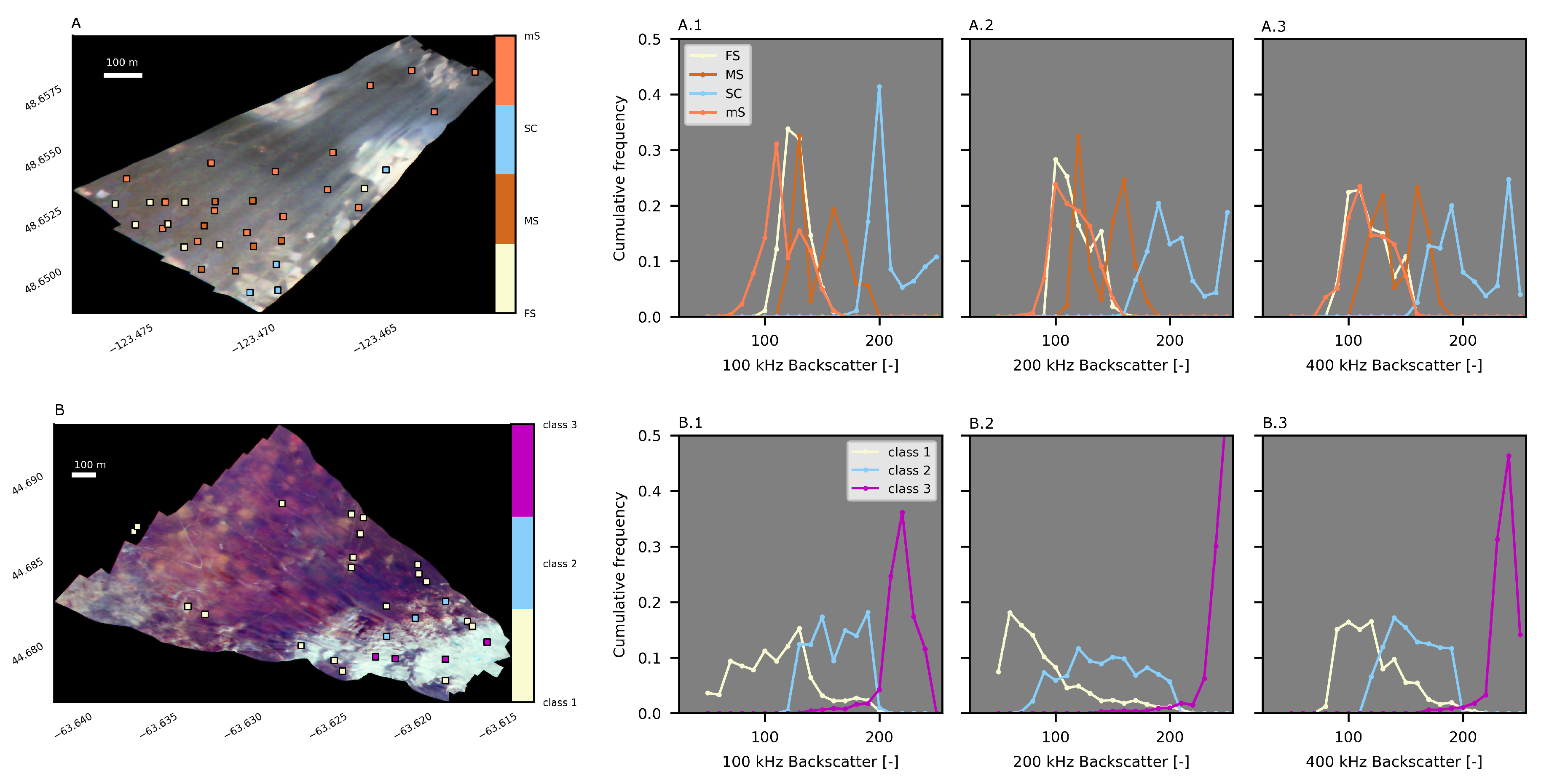
Frequency distributions of backscatter intensity were compiled based on locations of known substrate types (Figure 2A.1–A.3 for Patricia and Figure 2B.1–B.3 for Bedford). Despite the considerable amount of overlap between the resulting curves, which is partially a result of the inherently stochastic nature of backscatter [44] as well as the unaccounted-for variability within the substrate groups, the generally modest degree of separation between the peaks show that the task of using the GMM or CRF model for pixel-level substrate classification is, at the very least, analytically tractable. This analysis also serves to demonstrate the potential value of multispectral over monospectral backscatter. In a general sense, because each substrate has a different distribution of backscatter magnitude according to outgoing frequency, there is much more information for a probabilistic classifier to draw decision boundaries. For example, the backscatter associated with Bedford substrates Class 2 and Class 3 have a narrower range at high frequency compared to low, and all curves tend to be more multimodal at lower frequencies and more unimodal at higher frequencies. Further, the backscatter associated with Patricia Bay substrates mS and FS are only distinguishable at 100 kHz (Figure 2A.1).
3.2.1. GMM Model Implementation Details
Following [7], the GMM model was initialized using the observed per-substrate mean backscatter for , and unit weight and covariance . Model fitting continued until a convergence criterion was satisfied, which in the present study was when the average gain in posterior probability from the previous iteration went below 0.01.
The number of Gaussians may be optimized using the data (see [6,7] for two different approaches). In the present study, however, in order to keep the focus on the relative performance of the two models and the two types of backscatter (monospectral and multispectral), the number of modeled Gaussians in the mixture was set to equal the number of substrates known to be present in the surveyed area (four for Patricia, and three for Bedford). Any posterior probability below a certain threshold was reclassified as ‘unknown’ substrate. This threshold was arbitrarily set to 0.8 for all data sets. A 50% subsample of the bed observations, drawn at random but with the condition that at least one bed observation per class was included, was used to train the model. The remaining 50% of the bed observations were used to test the performance of the substrate classification model.
3.2.2. CRF Model Implementation Details
To explore the sensitivity of the CRF model to , keeping constant at a value of 100, the model was run using 10 equal-increment values between 30 and 800, using multispectral backscatter, and the results evaluated. Once the appropriate value for across all data sets had been decided and fixed, the model was run using equal-increment 10 values of Potts compatibility parameter between 3 and 300. In these tests, all inference algorithms were run for 30 iterations. Once the appropriate value for across all data sets had been decided and fixed, we explored the effects of number of inference iterations, from 1 to 20. Average posterior probabilities at the final model iteration tended to be very high for the CRF model. Therefore, in the sensitivity tests involving varying and parameters we instead used per-pixel posterior probabilities averaged over all model iterations, which was a more conservative estimate of probability being, for each pixel, a function of the rate of convergence to the final posterior probability, and therefore showed greater variability across entire ranges of parameter values.
Like in the GMM model, the final CRF model used a 50% subsample of the bed observations, drawn at random but with the condition that at least one bed observation per class was included, to train the model. The remaining 50% of the bed observations were used to test the performance of the substrate classification model. In all model runs except those with fewer bed observations, any posterior probability below a certain threshold was reclassified as ‘unknown’ substrate. For consistency with the GMM model, this threshold was set to 0.8.
3.2.3. Model Evaluation
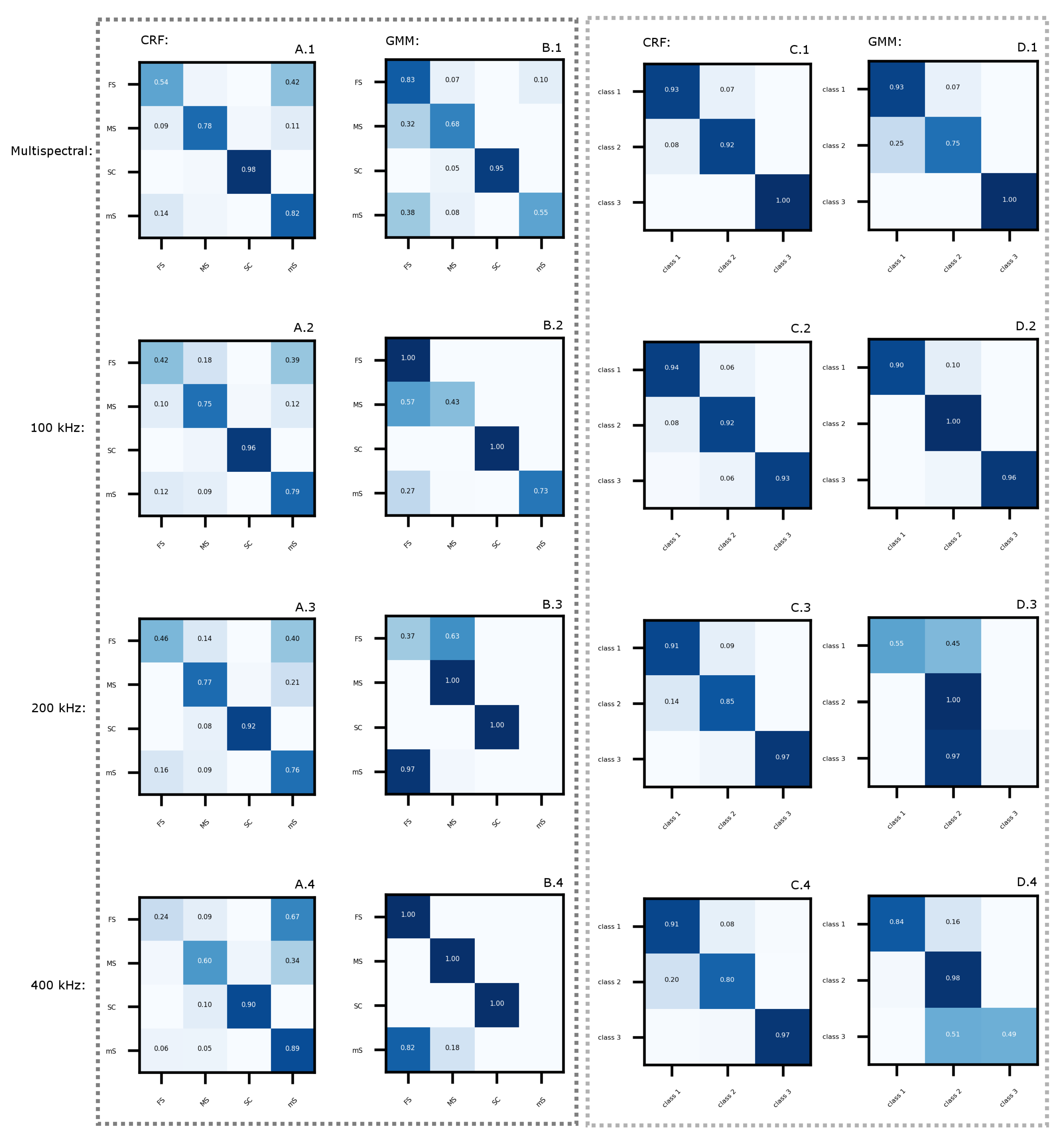
Each model was trained using a 50% subsample of the bed observations, drawn at random but with the condition that at least one bed observation per class was included. The remaining 50% of the bed observations were used to test the performance. Any posterior probability below 0.8 was reclassified as ‘unknown’ substrate. A ‘confusion matrix’, which is the matrix of normalized correspondences between true and estimated labels is used to visualize model skill. A perfect correspondence between true and estimated labels is scored 1.0 along the diagonal elements of the matrix. Misclassifications are readily identified as off-diagonal elements. Systematic misclassifications are recognized as off-diagonal elements with large magnitudes.
We also performed leave-one-out cross-validation for multispectral inputs whereby, upon successive iterations, one bed observation is randomly removed and a previously removed observation is replaced, and the model refitted. We did this for each site and each model: 35 iterations for Patricia and 27 iterations for Bedford, corresponding to the number of bed observations stations at each site. This procedure checks how well a model generalizes to data, by examining the variability in each classified grid cell over those many iterations, and also provides a means to examine spatially which areas of the bed were sensitive to a lack of ground truth bed observation. Such information could be used, for example, to target further bed sampling.
4. Results
4.1. Conditional Random Field (CRF) Model: Sensitivity to and
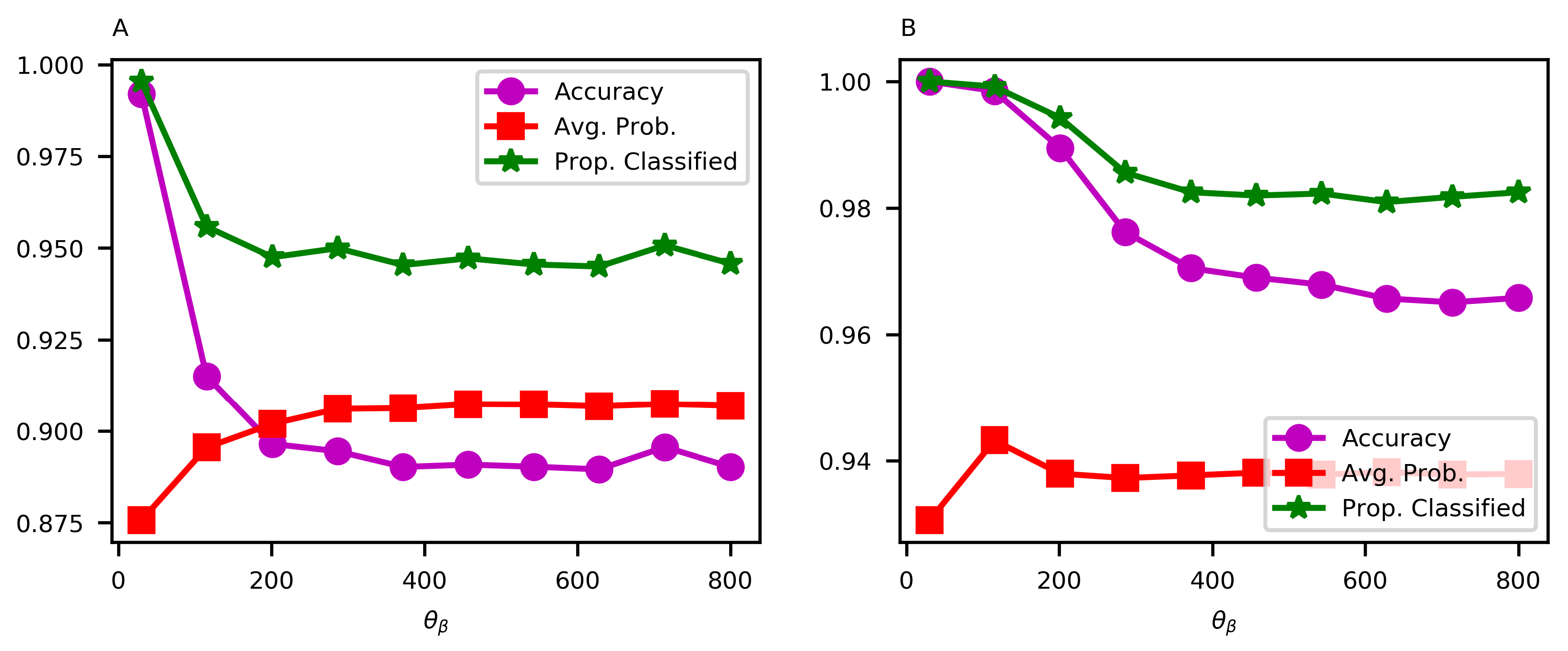
The parameter controls the degree of allowable similarity in backscatter between CRF graph nodes. Relatively large means backscatter features with relatively large differences in magnitude are assigned the same substrate label. The response of was not sensitive to value of . For each, three metrics were computed: (1) Accuracy (the number of correctly labeled pixels divided by the number of all tested pixels), (2) average posterior probability, and (3) proportion of the pixels with posterior probabilities > 0.8. An appropriate value for was considered to be one at which all three metrics stabilized. Accuracy is based on comparing pixels with known and model-predicted labels. When is small, accuracies (determined only at those calibration locations within the vicinity of available observations of the bed) are spuriously high because the average probability across the entire survey (i.e., in areas in and outside of the calibration) may be relatively low. As increases, accuracy and percent classified both tend to slightly decrease, stabilizing at uncertainty values that are more realistic given the observed variability in backscatter vectors (Figure 3). Based on the above criteria, across data from both sites, the appropriate value was determined to be .
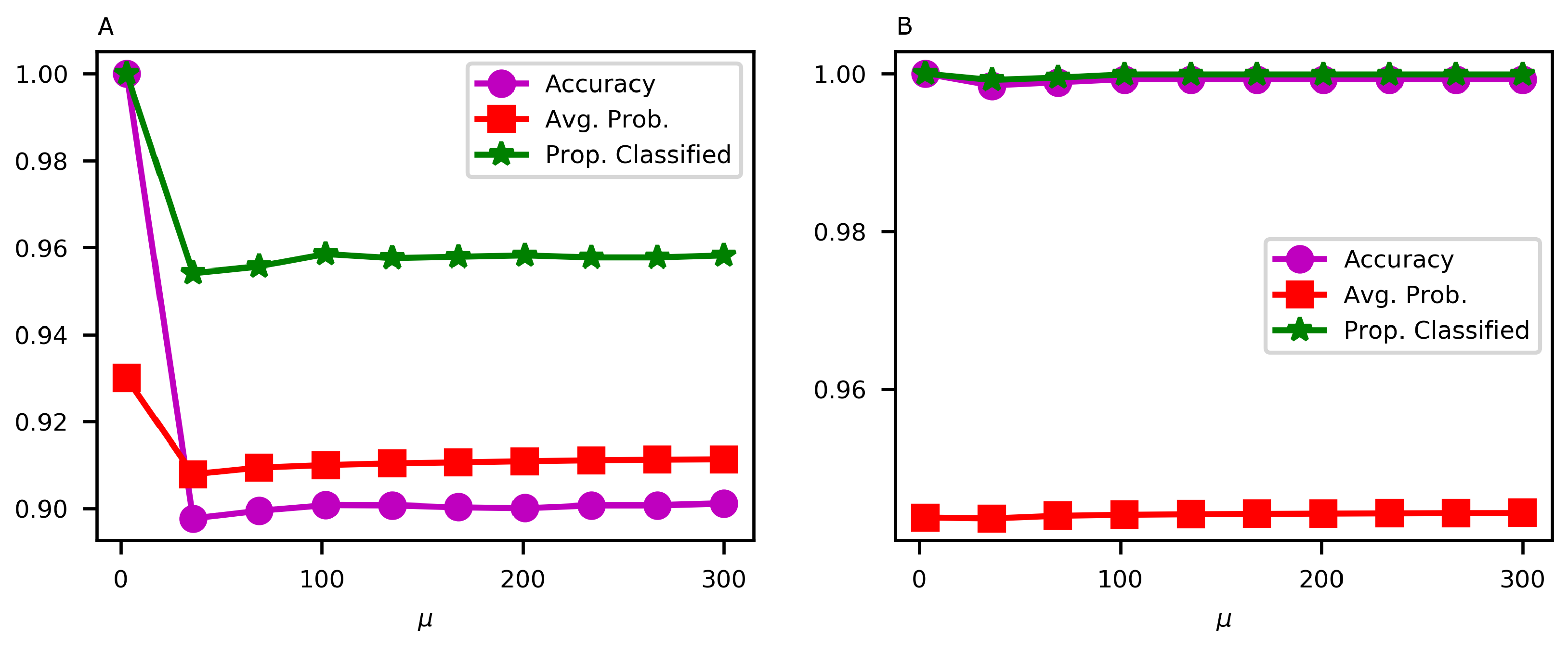
The compatibility function imposes a penalty for grid nodes that have similar backscattering but are assigned different labels, up to a distance of . This ‘proximity tolerance’ parameter therefore specifies the distance between pairs of pixels beyond which they are considered far enough apart to have similar backscattering but different substrate labels. The model was run using 10 equal-increment values of between 3 and 300 (Figure 4). The optimal value of was determined by the same criteria used to determine .
4.2. CRF: Number of Iterations
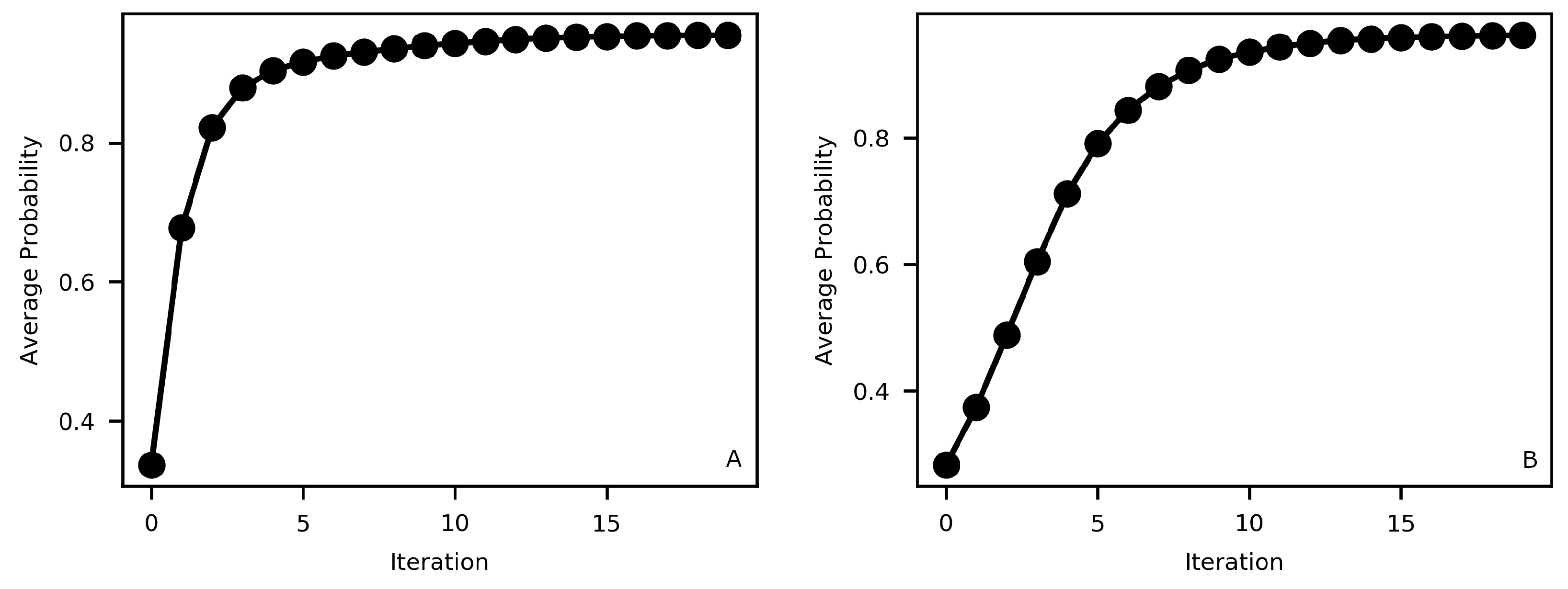
The effect of the number of CRF model iterations of the classification result was evaluated using average posterior probability as a metric. From the above, with = 300 and = 100, the number of iterations was increased from 1 to 20, in increments of 1. Average probability rapidly increases from 1 to 5 iterations, stabilizing beyond approximately 10 iterations (Figure 5). The speed with which average posterior probabilities stabilize (convergence rate) seems to be related to the spatial density of bed observations, with Patricia having the greatest spatial density of bed observations and the fastest convergence rate, and Bedford having the lower spatial density of bed observations and correspondingly the lower convergence rate (Figure 5).
4.3. Patricia Bay Substrate Classification
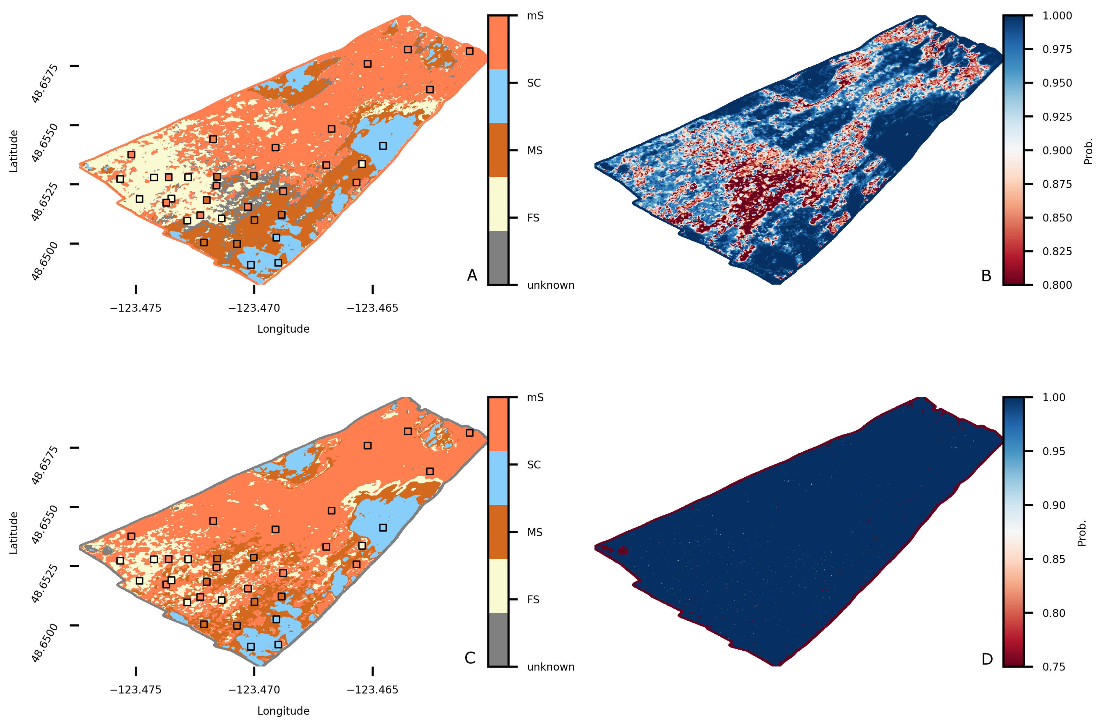
The GMM approach was used to generate, from multispectral backscatter inputs, a substrate classification map (Figure 6A) and associated map of prediction probabilities (Figure 6B). Using optimal settings ( = 300, = 100, and 15 iterations), the CRF approach was also used to generate a substrate classification map (Figure 6C) and associated map of prediction probabilities (Figure 6D) using multispectral data. In all cases, there is excellent qualitative correspondence between substrate patches and their nearby bed observations. Scrutiny of Figure 6A,C reveals that the greatest differences between substrate maps was in the FS class, which had an overall greater extent in the GMM prediction (Figure 6A). The other significant difference between the two approaches was the maps of prediction probabilities (Figure 6B,D), which tended to be far higher for the CRF model (Figure 6D). Rather than being an advantageous aspect of the CRF prediction, we suggest that those probabilities are not particularly useful for assessing the spatial variability in the quality of substrate predictions.
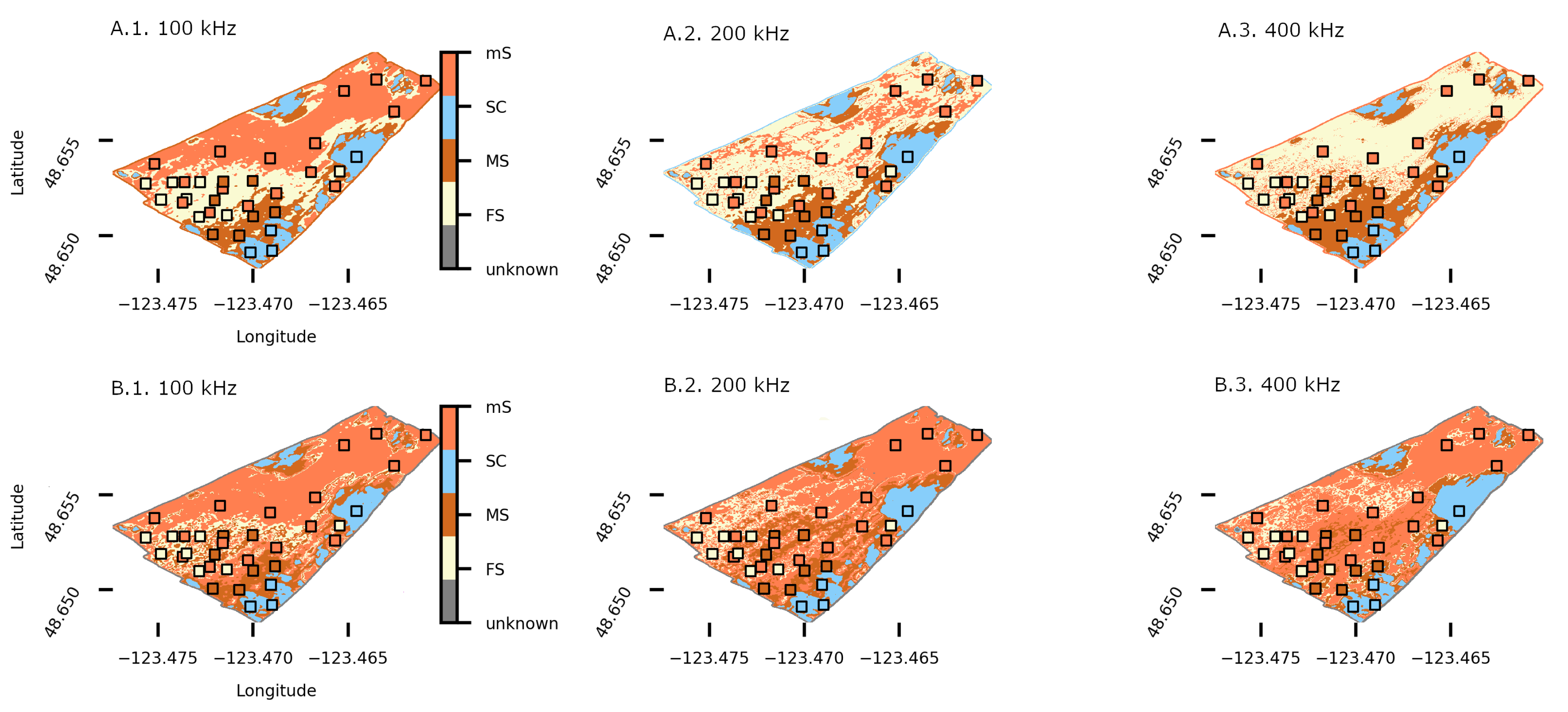
The GMM and CRF approaches were also used to generate substrate classification maps (Figure 7), using each of the three monospectral bands separately as inputs. There is generally a much greater propensity for the GMM model to (over-) predict the FS class (Figure 7A.1–A.3) because the GMM model takes into account only relative backscatter magnitudes, not their relative spatial locations like the CRF model does.
4.4. Bedford Basin Substrate Classification
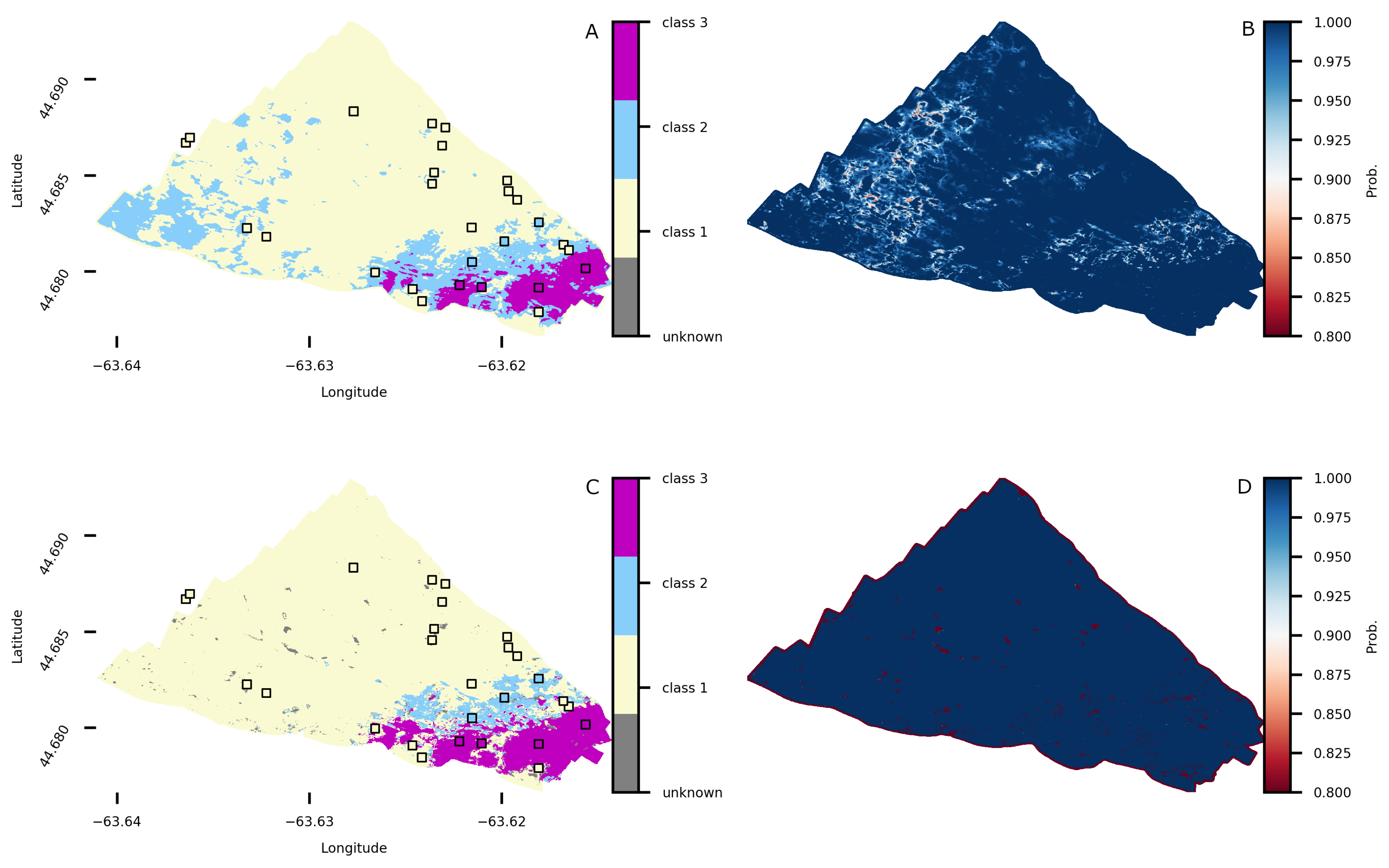
Like at the Patricia Bay site, both the GMM and CRF approaches were used to generate substrate classification maps (Figure 8A,C) and associated maps of prediction probabilities (Figure 8B,D).
The most noteworthy difference between the two model outputs is that the GMM model predicted a greater spatial extent of Class 2 substrates (Figure 8A) compared to the CRF model. This seems plausible considering that these areas correspond to relatively large magnitude backscattering (the western end of Figure 2A) across all three spectral bands. It seems likely that the CRF model penalized the prediction of Class 2 in this area because of its large distance to any Class 2 bed observations. Unfortunately, it is impossible to say whether the GMM or the CRF model was correct in this instance there is no ground truth information in this area; supervised models can only be evaluated based on how well they predict known substrate classes.
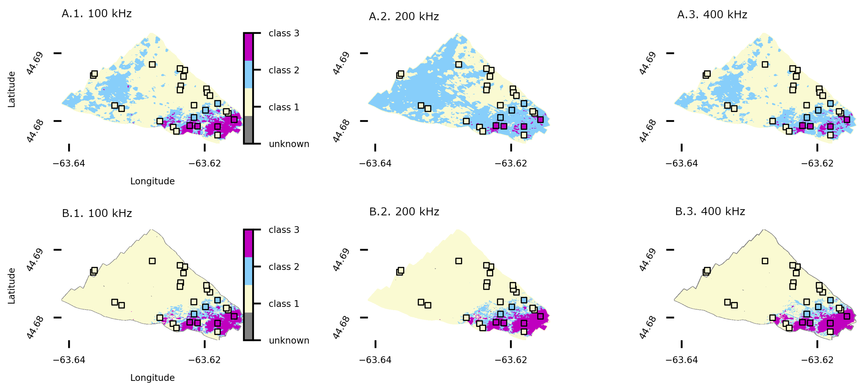
Like at Patricia Bay, the GMM and CRF approaches were also used to generate substrate classification maps (Figure 9), using each of the three monospectral bands separately as inputs. Once again, there is generally a much greater propensity for the GMM model to (over-) predict a certain class, this time Class 2 (Figure 9A.1–A.3), especially at 200 kHz. It seems likely that the GMM model assigns spuriously high weights to this intermediate substrate class because the simple covariance structure of the model is unable to capture the correlations between the two end member substrate classes, therefore the intermediate class becomes a ‘probability sink’. Like at Patricia Bay, the CRF-derived substrate maps are spatially more homogeneous because the relative spatial locations of the bed observations are given weighting comparable to that given to relative differences in backscattering magnitude. At both sites, the relative spatial homogeneity of CRF-predicted classes seems more physically plausible than the relative heterogeneity of the GMM predictions. That is not to say that such variability in substrates is not real: In fact, it is entirely possible that the acoustic variability is due to variability in substrate composition that is not adequately captured by the few classes that all bed observations were grouped into. However, given the limited number of substrate classes, the GMM models have ‘over-fit’ [23] the backscatter data, capturing acoustic variability as substrate variability, unfiltered by the strong effects of spatial autocorrelation over the substrate, which is picked up well by the CRF model.
4.5. Synthesis of All Model Results
The model synthesis shown in Figure 10 and described below uses 50% of the bed observations to test the performance. At Patricia Bay, the average CRF classification accuracy across all three substrate types was 78% using multispectral inputs (Figure 10A.1), compared to 75% for the GMM model (Figure 10B.1). Using monospectral backscatter inputs of 100, 200, and 400 kHz, average CRF classification accuracies were respectively 73%, 73%, and 66% (Figure 10A.2–A.4). Corresponding GMM classification accuracies were respectively 79%, 59%, and 75% (Figure 10B.2–B.4). At Bedford, the average CRF classification accuracy across all three substrate types was 95% using multispectral inputs (Figure 10C.1), compared to 89% for the GMM model (Figure 10D.1). Using monospectral backscatter inputs of 100, 200, and 400 kHz, average CRF classification accuracies were respectively 93%, 91%, and 89% (Figure 10C.2–C.4). Corresponding GMM classification accuracies were respectively 95%, 52%, and 77% (Figure 10D.2–D.4).
Overall, therefore, the CRF performed significantly better than the GMM model at both sites with multispectral backscatter inputs. For monospectral inputs, the CRF performed significantly better than the GMM model at Bedford (91% versus 75% overall accuracy for CRF and GMM models, respectively) whereas the differences were negligible at Patricia Bay (70.5% versus 71% overall accuracy for CRF and GMM models, respectively). Care must be taken to interpret these task-specific classification results in physical terms. For example, these results do not necessarily reflect the relative importance (or, strictly speaking, information content) of each acoustic frequency compared to multispectral backscatter, because the relative contributions of the different frequencies to overall model performance would not be linear, nor additive.
At Patricia Bay, the leave-one-out cross-validation procedure carried out on the on the CRF map was a 91% mean accuracy across all four substrate classes. The maximum variability in accuracy between folds was largest (6.1%) for the FS class and relatively small for class MS (3.9%), SC (2.3%), and class mS (0.07%). The GMM result was significantly worse: 65% mean accuracy across all four substrate classes with variability in accuracy between folds between 20 and 39% depending on the class. At Bedford Basin, the CRF result was a 99.5% mean accuracy across all three substrate classes. The maximum variability in accuracy between folds was largest (2.9%) for Class 2 and relatively small for Class 1 (1.53%) and Class 3 (1.47%). The GMM result was 84% mean accuracy across all substrate classes with variability in accuracy between folds between 4 and 16% depending on the class.
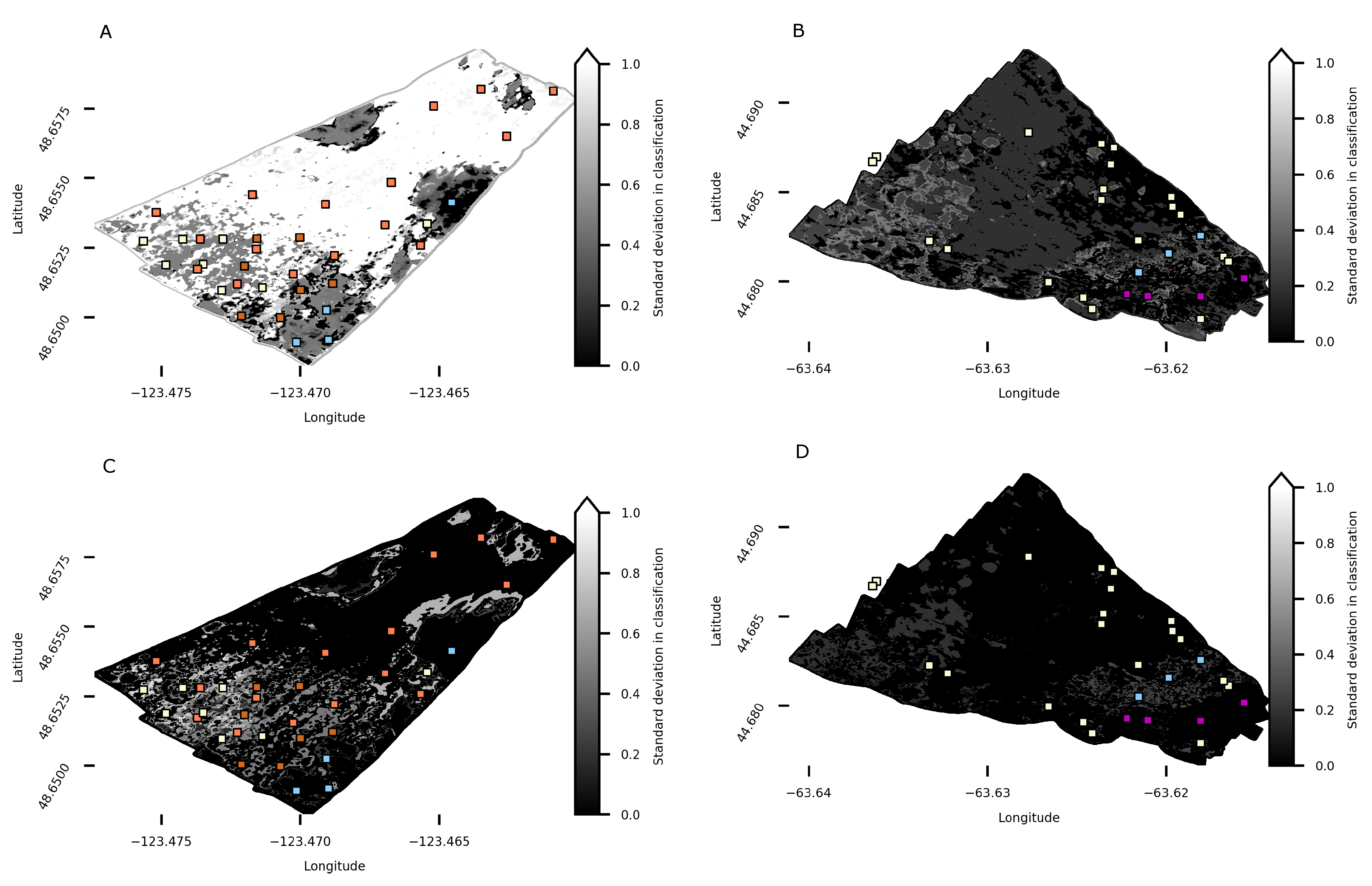
Overall, the CRF model creates outputs that are much less sensitive to the number and location of bed observations, compared with the GMM model, which suggests that the CRF model generalizes to data much better. The standard deviations in bed classifications (Figure 11) show that, at both sites, the GMM model was much more sensitive to the presence and location of individual bed observations, especially at Patricia Bay (Figure 11A). The CRF model is much less sensitive (standard deviation in classifications are much lower), owing to its ability to incorporate spatial autocorrelation in substrates as well as relative differences in backscattering magnitude.
5. Discussion and Conclusions
We suggest that the high classification accuracies and probabilities of the CRF model outputs were the result of that model incorporating spatial information, as well as backscatter magnitudes, through the use of pairwise potentials that quantify the computational cost of simultaneously assigning label to grid node i and to grid node j (10), parameterized using a ‘proximity tolerance’ parameter . It is encouraging that substrate classification outputs were not overly sensitive to parameter values (Figure 3 and Figure 4), at least beyond a certain low value. Collectively, this suggests that CRF models applied elsewhere might use similar values for , which controls the degree of allowable similarity in backscatter between graph nodes, and . Model parameters and have clear physical meaning and are related to physical proximity and backscatter similarity, respectively. The model might be further extended by adding a kernel to (11) that captures only the spatial proximity of features, with a parameter controlling the degree of allowable similarity in position between graph nodes. The ‘Potts model’ for label compatibility is oversimplistic because it penalizes a pair of nearby grid nodes the same irrespective of their labels. Compatibility functions that learn from the data could be implemented using methods discussed by [37], whereby substrates that are physically likely to be proximal are penalized less than those unlikely to be nearby.
The CRF is analytically more complicated than other discriminative approaches, however, owing to the implementation of an efficient inference algorithm [35], the added computational cost is negligible. Among discriminative approaches, which also include support vector machines [19], decision trees [20,26], neural networks [25], and random forests [27], among others, there are many potential advantages to the CRF. The biggest advantage is that a CRF model does not need to make independence assumptions about the data, or model the correlations between substrate features, to learn a discriminant function that best maps inputs x directly into labels y. This is especially important for use with emerging multispectral sonar technology because, until it is understood how substrates respond quantitatively to multiple frequencies, we require a substrate model that does not rely on a statistical assumption of independence, which says that the substrate features do not depend on and affect each other.
We used CRF models based on gridded backscatter magnitude only, purposefully ignoring other potentially useful derived products of bathymetry (depth, roughness, slope, aspect, curvature, etc), or backscatter [22]. While the CRF model can use features consisting of any number of spatially co-registered inputs, using backscatter alone demonstrates suitability for task-specific substrate classification without transforming the data into a chosen set of inputs amenable to a specific machine learning algorithm from among a set of candidate inputs. A disadvantage of this so-called feature engineering is that it makes it harder to evaluating the relative importance of all features that make up a given realization of , especially among disparate data sets. Using backscatter alone is relatively powerful, elegant and parsimonious.
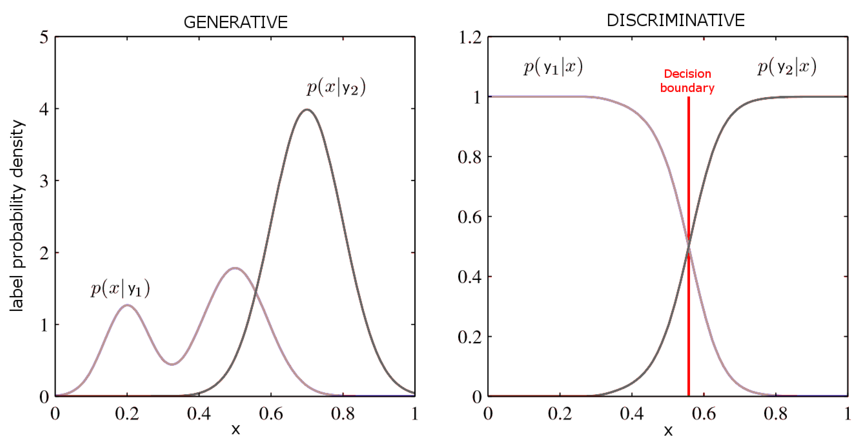
Generative approaches are statistically more complex, due to the added complexity of statistically modeling the specific joint probability of the substrate features (backscatter at frequency 1, frequency 2, etc) and their labels together, and make restrictive assumptions about the distribution of the data, such as independence assumptions between backscatter features given a label. As here, when the task requires only finding the posterior probabilities of substrates, that is the conditional distribution of y given , , generative models can be overly complicated and, in the words of [39], “excessively demanding of data”. The label-conditional probabilities may contain a lot of detail that is not used. An example of this is shown in Figure 12 in which the left-hand mode of substrate in the left plot has no effect on the corresponding posterior probability in the right plot. Compare the multiple modes in the label-conditional probabilities shown in Figure 2, where we may also observe that the label-conditional density assumptions of the GMM, namely, that each class may be modeled as a Gaussian—that is, a unimodal function—gave a comparatively poor approximation to the true distributions.
However, generative models are by definition more powerful when direct observations of the bed are relatively scarce: If the joint probability distribution function is statistically well behaved, given a particular y, you can then calculate (or ‘generate’) its respective . For generative models, therefore, the training set in theory can contain data from multiple sites and times. If the generative model is sufficiently broad in scope, it can be applied to areas of the substrate with no bed observations, whereas the discriminative approach tends to rely on bed observations from within the area mapped by the sonar. Thus far, however, in practice this tends not to be the case. In other words, models to estimate substrates tend to be built for specific sites and are not typically transferred between sites without recalibration or reparameterization, and the practical scope of generative and discriminative models has become similar. In the longer term, this situation may change, and generative models may be more widely applicable outside of their calibration. Until that time, however, we predict that discriminative models will remain a popular and useful approach to task-specific substrate classification, especially if they better model spatial dependencies, such as the CRF. Given the relative advantages of both model types, there has long been interest in a hybrid approach [45], which is perhaps now on the horizon with the discovery of the generative applications [46] of deep neural networks [33,47] which, to our knowledge, have yet to be applied to substrate characterization but would be an interesting and potentially useful development.
References
Author Contributions
Conceptualization: D.B.; methodology: D.B. and P.G.; software: D.B.; validation: D.B. and P.G.; formal analysis: D.B.; data curation: D.B.; writing—original draft preparation: D.B. and P.G.; writing—review and editing: D.B. and P.G.; visualization: D.B.; and funding acquisition: D.B. and P.G.
Funding
This work was funded by the U.S. Geological Survey Grand Canyon Monitoring and the Research Center, by means of an award to Northern Arizona University (USGS Agreements G17AC00270).
Acknowledgments
All backscatter data were provided by R2Sonic, LLC (Austin, TX, USA) for the 2017 Multispectral Challenge. Any use of trade, product, or firm names is for descriptive purposes only and does not imply endorsement by the U.S. Government. These methods may be implemented using the PriSM toolbox (https://www.danielbuscombe.com/prism/), freely available at https://github.com/dbuscombe-usgs/prism.
Conflicts of Interest
The authors declare no conflict of interest.
References
- Kenny, A.; Cato, I.; Desprez, M.; Fader, G.; Schuttenhelm, R.; Side, J. An overview of seabed-mapping technologies in the context of marine habitat classification. ICES J. Mar. Sci. 2003, 60, 411–418. [Google Scholar] [CrossRef] [Green Version]
- Brown, C.; Smith, S.; Lawton, P.; Anderson, J. Benthic habitat mapping: A review of progress towards improved understanding of the spatial ecology of the substrate using acoustic techniques. Estuar. Coast. Shelf Sci. 2011, 92, 502–520. [Google Scholar] [CrossRef]
- Mayer, L.; Jakobsson, M.; Allen, G.; Dorschel, B.; Falconer, R.; Ferrini, V.; Lamarche, G.; Snaith, H.; Weatherall, P. The Nippon Foundation–GEBCO Seabed 2030 Project: The Quest to See the World’s Oceans Completely Mapped by 2030. Geosciences 2018, 8, 2. [Google Scholar] [CrossRef]
- Ierodiaconou, D.; Monk, J.; Rattray, A.; Laurenson, L.; Versace, V. Comparison of automated classification techniques for predicting benthic biological communities using hydroacoustics and video observations. Cont. Shelf Res. 2011, 31, S28–S38. [Google Scholar] [CrossRef]
- Harris, P.; Baker, E. Why map benthic habitats. In Substrate Geomorphology as Benthic Habitat; Elsevier: London, UK, 2012; pp. 3–22. [Google Scholar]
- Amiri-Simkooei, A.; Snellen, M.; Simons, D. Riverbed sediment classification using multi-beam echo-sounder backscatter data. J. Acoust. Soc. Am. 2009, 126, 1724–1738. [Google Scholar] [CrossRef] [PubMed]
- Buscombe, D.; Grams, P.; Kaplinski, M. Compositional signatures in acoustic backscatter over vegetated and unvegetated mixed sand-gravel riverbeds. J. Geophys. Res. Earth Surf. 2017, 122, 1771–1793. [Google Scholar] [CrossRef]
- Lamarche, G.; Lurton, X. Recommendations for improved and coherent acquisition and processing of backscatter data from substrate-mapping sonars. Mar. Geophys. Res. 2018, 39, 5–22. [Google Scholar] [CrossRef]
- Schimel, A.; Beaudoin, J.; Parnum, I.; le Bas, T.; Schmidt, V.; Keith, G.; Ierodiaconou, D. Multibeam sonar backscatter data processing. Mar. Geophys. Res. 2018, 39, 121–137. [Google Scholar] [CrossRef]
- Malik, M.; Lurton, X.; Mayer, L. A framework to quantify uncertainties of substrate backscatter from swath mapping echosounders. Mar. Geophys. Res. 2018, 39, 1–18. [Google Scholar] [CrossRef]
- Roche, M.; Degrendele, K.; Vrignaud, C.; Loyer, S.; le Bas, T.; Augustin, J.; Lurton, X. Control of the repeatability of high frequency multibeam echosounder backscatter by using natural reference areas. Mar. Geophys. Res. 2018, 39, 89–104. [Google Scholar] [CrossRef]
- Lecours, V.; Dolan, M.; Micallef, A.; Lucieer, V.L. A review of marine geomorphometry, the quantitative study of the substrate. Hydrol. Earth Syst. Sci. 2016, 20, 3207–3244. [Google Scholar] [CrossRef]
- Diesing, M.; Mitchell, P.; Stephens, D. Image-based seabed classification: What can we learn from terrestrial remote sensing? ICES J. Mar. Sci. 2016, 73, 2425–2441. [Google Scholar] [CrossRef]
- Jackson, D.; Winebrenner, D.; Ishmaru, A. Application of the composite roughness model to high frequency bottom backscattering. J. Acoust. Soc. Am. 1986, 79, 1410–1422. [Google Scholar] [CrossRef]
- Jackson, D.; Richardson, M. High-Frequency Substrate Acoustics, 1st ed.; Springer Science & Business Media: New York, NY, USA, 2007; p. 616. [Google Scholar]
- Kloser, R.; Penrose, J.; Butler, A. Multi-beam backscatter measurements used to infer seabed habitats. Cont. Shelf Res. 2010, 30, 1772–1782. [Google Scholar] [CrossRef]
- Jackson, D.; Briggs, K.; Williams, K.; Richardson, M. Tests of models for high-frequency substrate backscatter. IEEE J. Ocean. Eng. 1996, 21, 458–470. [Google Scholar] [CrossRef]
- Diesing, M.; Stephens, D. A multi-model ensemble approach to seabed mapping. J. Sea Res. 2015, 100, 62–69. [Google Scholar] [CrossRef]
- Stephens, D.; Diesing, M. A comparison of supervised classification methods for the prediction of substrate type using multibeam acoustic and legacy grain-size data. PLoS ONE 2014, 9, e93950. [Google Scholar] [CrossRef] [PubMed]
- Dartnell, P.; Gardner, J. Predicting substrate facies from multibeam bathymetry and backscatter data. Photogramm. Eng. Remote. Sens. 2004, 70, 1081–1091. [Google Scholar] [CrossRef]
- Huvenne, V.; Robert, K.; Marsh, L.; Iacono, C.; le Bas, T.; Wynn, R. ROVs and AUVs. In Submarine Geomorphology; Springer: Berlin/Heidelberg, Germany, 2018; pp. 93–108. [Google Scholar]
- Buscombe, D.; Grams, P.; Kaplinski, M. Characterizing riverbed sediments using high-frequency acoustics 1: Spectral properties of scattering. J. Geophys. Res. Earth Surf. 2014, 119, 2674–2691. [Google Scholar] [CrossRef]
- Murphy, K. Machine Learning: A Probabilistic Perspective; MIT Press: Cambridge, UK, 2012. [Google Scholar]
- Simons, D.; Snellen, M. A Bayesian approach to substrate classification using multi-beam echo-sounder backscatter data. Appl. Acoust. 2009, 70, 1258–1268. [Google Scholar] [CrossRef]
- Marsh, I.; Brown, C. Neural network classification of multibeam backscatter and bathymetry data from Stanton Bank (Area IV). Appl. Acoust. 2009, 70, 1269–1276. [Google Scholar] [CrossRef]
- Buscombe, D.; Grams, P.; Kaplinski, M. Characterizing riverbed sediments using high-frequency acoustics 2: Scattering signatures of Colorado River bed sediments in Marble and Grand Canyons. J. Geophys. Res. Earth Surf. 2014, 119, 2692–2710. [Google Scholar] [CrossRef]
- Lucieer, V.; Hill, N.; Barrett, N.; Nichol, S. Do marine substrates ‘look’ and ‘sound’ the same? Supervised classification of multibeam acoustic data using autonomous underwater vehicle images. Estuar. Coast. Shelf Sci. 2013, 117, 94–106. [Google Scholar] [CrossRef]
- Beaudoin, J.; Clarke, J.H.; Doucet, M.; Brown, C.; Brissette, M.; Gazzola, V. Setting the Stage for Multispectral Acoustic Backscatter Research; GeoHab: Winchester, UK, 2016. [Google Scholar]
- Feldens, P.; Schulze, I.; Papenmeier, S.; Schönke, M.; von Deimling, J.S. Improved Interpretation of Marine Sedimentary Environments Using Multi-Frequency Multibeam Backscatter Data. Geosciences 2018, 8, 214. [Google Scholar] [CrossRef]
- Koller, D.; Friedman, N. Probabilistic Graphical Models: Principles and Techniques; MIT Press: Cambridge, UK, 2009; pp. 104–109. [Google Scholar]
- Lafferty, J.; McCallum, A.; Pereira, F. Conditional random fields: Probabilistic models for segmenting and labeling sequence data. Int. Conf. Mach. Learn. (ICML) 2001, 282–289. [Google Scholar]
- Zhu, H.; Meng, F.; Cai, J.; Lu, S. Beyond pixels: A comprehensive survey from bottom-up to semantic image segmentation and cosegmentation. J. Vis. Commun. Image Represent. 2016, 34, 12–27. [Google Scholar] [CrossRef] [Green Version]
- Buscombe, D.; Ritchie, A.C. Landscape Classification with Deep Neural Networks. Geosciences 2018, 8, 244. [Google Scholar] [CrossRef]
- Kumar, S.; Hebert, M. Discriminative random fields. Int. J. Comput. Vision 2006, 68, 179–201. [Google Scholar] [CrossRef]
- Krähenbühl, P.; Koltu, V.N. Efficient inference in fully connected CRFs with Gaussian edge potentials. In Advances in Neural Information Processing Systems; Neural Information Processing Systems Foundation, Inc.: Granada, Spain, 2011; pp. 109–117. [Google Scholar]
- Tappen, M.; Liu, C.; Adelson, E.; Freeman, W. Learning Gaussian conditional random fields for low-level vision. In Proceedings of the IEEE Conference on Computer Vision and Pattern Recognition, Minneapolis, MN, USA, 17–22 June 2007; pp. 1–8. [Google Scholar]
- Krähenbühl, P.; Koltun, V. Parameter learning and convergent inference for dense random fields. In Proceedings of the International Conference on Machine Learning, Atlanta, CA, USA, 16–21 June 2013; pp. 513–521. [Google Scholar]
- Hamill, D.; Buscombe, D.; Wheaton, J.M. Alluvial substrate mapping by automated texture segmentation of recreational-grade side scan sonar imagery. PLoS ONE 2018, 13, e0194373. [Google Scholar] [CrossRef] [PubMed]
- Bishop, C. Pattern Recognition and Machine Learning; Springer Science and Business Media: New York, NY, USA, 2006. [Google Scholar]
- Ainslie, M.; McColm, J. A simplified formula for viscous and chemical absorption in sea water. J. Acoust. Soc. Am. 1998, 103, 1671–1672. [Google Scholar] [CrossRef]
- Fader, G.B.J.; Miller, R.O. Surficial geology, Halifax Harbour, Nova Scotia. Bull. Geol. Surv. Can. 2008, 590, 163. [Google Scholar]
- Biffard, B. Seabed Remote Sensing by Single-Beam Echosounder: Models, Methods and Applications. Ph.D. Thesis, University of Victoria, Victoria, BC, Canada, 2011. [Google Scholar]
- Brown, C.; Varma, H.; Multispectral Seafloor Classification: Applying a Multidimensional Hypercube Approach to Unsupervised Seafloor Segmentation. R2Sonic Multispectral Backscatter Competition Entry. Available online: https://www.r2sonic.com/geohab2018/ (accessed on 10 January 2018).
- Gavrilov, A.; Parnum, I. Fluctuations of substrate backscatter data from multibeam sonar systems. IEEE J. Ocean. Eng. 2010, 35, 209–219. [Google Scholar] [CrossRef]
- Lasserre, J.; Bishop, C.; Minka, T. Principled hybrids of generative and discriminative models. IEEE. Conf. Comp. Vision (CVPR) 2006, 1, 87–94. [Google Scholar]
- Goodfellow, I.; Pouget-Abadie, J.; Mirza, M.; Xu, B.; Warde-Farley, D.; Ozair, S.; Courville, A.; Bengio, Y. Generative adversarial nets. Adv. Neur. Inf. Process. Syst. 2014, 2672–2680. [Google Scholar]
- LeCun, Y.; Bengio, Y.; Hinton, G. Deep learning. Nature 2015, 521, 436. [Google Scholar] [CrossRef] [PubMed]
Figure 1.
Schematic of generative versus discriminative approaches to probabilistic substrate classification. Both approaches train a model from the data that make optimal label assignments. The generative approach first models the label-conditioned probabilities () for each label class individually, or joint distribution () between substrate features and substrate types (labels), then finds the posterior probabilities of each label (). The discriminative approach learns a decision boundary (or discriminant function) between labels that maps substrate features directly into labels.

Figure 2.
(A,B) (Patricia and Bedford sites, respectively): False color image with red, green, and blue values of each pixel corresponding to 8-bit values of backscattering strength at, respectively, 100, 200, and 400 kHz outgoing acoustic frequencies. Overlain are the locations of bed observations, color-coded according to the legend. At Patricia, the substrate classes are fine sand (FS), muddy sand (MS), sand/cobble (SC), and sandy mud (mS). At Bedford, Class 1 is mud; Class 2 is cobbles and boulders with interstitial mud; and Class 3 is cobbles, gravel, and boulders. A1–A3 and B1–B3 (Patricia and Bedford sites, respectively): Normalized non-dimensional [-] frequency distributions of 8-bit digital integers of backscatter intensity, compiled based on locations of known substrate types. From left to right: Response at 100, 200, and 400 kHz, respectively.

Figure 3.
Accuracy, average posterior probability, and proportion classified as a function of , for Patricia (A) and Bedford (B) datasets.
Figure 3.
Accuracy, average posterior probability, and proportion classified as a function of , for Patricia (A) and Bedford (B) datasets.

Figure 4.
Accuracy, average posterior probability, and proportion classified as a function of , for Patricia (A) and Bedford (B) datasets.
Figure 4.
Accuracy, average posterior probability, and proportion classified as a function of , for Patricia (A) and Bedford (B) datasets.

Figure 5.
Average conditional random field (CRF) posterior probability as a function of iteration, for the Patricia (A) and Bedford (B) sites.
Figure 5.
Average conditional random field (CRF) posterior probability as a function of iteration, for the Patricia (A) and Bedford (B) sites.

Figure 6.
Substrate classification using multispectral Patricia Bay data. Top row: Substrate map (A) and associated probability (B) using the Gaussian Mixture Model (GMM) algorithm. Bottom row: Substrate map (C) and associated probability (D) using the CRF algorithm.
Figure 6.
Substrate classification using multispectral Patricia Bay data. Top row: Substrate map (A) and associated probability (B) using the Gaussian Mixture Model (GMM) algorithm. Bottom row: Substrate map (C) and associated probability (D) using the CRF algorithm.

Figure 7.
Substrate classification using monospectral Patricia Bay data. Top row (A.1–A.3): Substrate maps generated with the GMM algorithm using 100, 200, or 400 kHz backscatter inputs. Bottom row: (B.1–B.3): Substrate maps generated with the CRF algorithm using 100, 200, or 400 kHz backscatter inputs.

Figure 8.
Substrate classification using multispectral Bedford Basin data. Top row: Substrate map (A) and associated probability (B) using the GMM algorithm. Bottom row: Substrate map (C) and associated probability (D) using the CRF algorithm.
Figure 8.
Substrate classification using multispectral Bedford Basin data. Top row: Substrate map (A) and associated probability (B) using the GMM algorithm. Bottom row: Substrate map (C) and associated probability (D) using the CRF algorithm.

Figure 9.
Substrate classification using monospectral Bedford Basin data. Top row (A.1–A.3): Substrate maps generated with the GMM algorithm using 100, 200, or 400 kHz backscatter inputs. Bottom row: (B.1–B.3): Substrate maps generated with the CRF algorithm using 100, 200 or 400 kHz backscatter inputs.

Figure 10.
Confusion matrices for CRF and GMM-derived substrate classifications, for Patricia (A,B) and Bedford (C,D) sites. Rows, from top to bottom, indicate multispectral, 100 kHz, 200 kHz, and 400 kHz inputs, respectively. Columns, from left to right, indicate Patricia/CRF, Patricia/GMM, Bedford/CRF, and Bedford/GMM, respectively. The numbers in each cell indicate the proportion of all classifications for each class.

Figure 11.
Standard deviation in substrate classifications computed using 35 and 27 realizations of model outputs at Patricia (A,C) and Bedford (B,D), respectively. The top row shows results from GMM outputs, and the bottom row shows CRF outputs. Each realization was based on a 1 fewer bed observation than the full set, drawn randomly. The bed observations are shown for reference.

Figure 12.
Example of label-conditional probability densities (left) for two substrates, and , as a function of a single substrate feature, , and the corresponding posterior probabilities (right). The vertical line in the right plot shows the discriminative decision boundary. Notice that the left-hand mode of substrate in the left plot has no effect on the corresponding posterior probability in the right plot. Figure modified from [39].


Table 1.
Acoustic Processing Parameters.
| Patricia Bay | Bedford | |
|---|---|---|
| absorption @ 100 kHz [dB/km] | 28.9 | 23.1 |
| absorption @ 200 kHz [dB/km] | 48.4 | 39.3 |
| absorption @ 400 kHz [dB/km] | 89.1 | 91.7 |
| response @ 100 kHz [dB] | 25.6 | 23.6 |
| response @ 200 kHz [dB] | 12.9 | 12.9 |
| response @ 400 kHz [dB] | 4.8 | 4.8 |
© 2018 by the authors. Licensee MDPI, Basel, Switzerland. This article is an open access article distributed under the terms and conditions of the Creative Commons Attribution (CC BY) license (http://creativecommons.org/licenses/by/4.0/).
Share and Cite
MDPI and ACS Style
Buscombe, D.; Grams, P.E. Probabilistic Substrate Classification with Multispectral Acoustic Backscatter: A Comparison of Discriminative and Generative Models. Geosciences 2018, 8, 395. https://doi.org/10.3390/geosciences8110395
AMA Style
Buscombe D, Grams PE. Probabilistic Substrate Classification with Multispectral Acoustic Backscatter: A Comparison of Discriminative and Generative Models. Geosciences. 2018; 8(11):395. https://doi.org/10.3390/geosciences8110395
Chicago/Turabian StyleBuscombe, Daniel, and Paul E. Grams. 2018. "Probabilistic Substrate Classification with Multispectral Acoustic Backscatter: A Comparison of Discriminative and Generative Models" Geosciences 8, no. 11: 395. https://doi.org/10.3390/geosciences8110395
Note that from the first issue of 2016, this journal uses article numbers instead of page numbers. See further details here.