Comparison of the Sweetness Seismic Attribute and Porosity–Thickness Maps, Sava Depression, Croatia

1
INA Plc., Avenija Većeslava Holjevca 10, 10000 Zagreb, Croatia
2
Faculty of Mining, Geology and Petroleum Engineering, University of Zagreb, Pierottijeva 6, 10000 Zagreb, Croatia
*
Author to whom correspondence should be addressed.
Geosciences 2018, 8(11), 426; https://doi.org/10.3390/geosciences8110426
Submission received: 6 September 2018
/
Revised: 6 November 2018
/
Accepted: 16 November 2018
/
Published: 21 November 2018
(This article belongs to the Special Issue Geostatistical Applications in Petroleum Geology)
Abstract
:The sweetness seismic attribute is a very useful tool for proper description of the depositional environment, reservoir quality and lithofacies discrimination. This paper shows that depositional channels and turbidity sandstones deposited during the Upper Pannonian and Lower Pontian in the Sava Depression can be described using porosity–thickness and sweetness seismic attribute maps. Two studied reservoirs are of Neogene stage (“UP” reservoir of Upper Pannonian age and “LP” reservoir of Lower Pontian age) and located in the Sava Depression, Croatia. Both reservoirs contain medium to fine grained sandstones that are intercalated with basinal marls. A comparison of the sweetness seismic attribute and porosity–thickness maps show a good visual match with correlation coefficient of approximately 0.85. A mismatch was observed in areas with small reservoir thickness. This work demonstrates the importance of using porosity–thickness maps for reservoir characterization. The workflow presented in this work has wider applications in frontier areas with poor seismic data or coverage.
1. Introduction
A description of the depositional environments of turbidite reservoirs is necessary for field development. If the hydrocarbon reservoirs are in the final stage of production, knowledge of the reservoir itself must be completely thorough. This is very important because in that way, residual hydrocarbon saturation can be defined in a way to assume that fluid contacts will rise rapidly in the channel center with better properties than in the channel lobes with low porosities and permeabilities.
The use of seismic attribute for reservoir and geomorphological characterization are well described in several papers [1,2,3,4]. Three dimensional (3D) seismic data and seismic attribute are frequently used for proper description of the depositional environment, reservoir quality and lithofacies discrimination in combination with well log data [5,6]. Of importance is sweetness seismic attribute as a very useful tool for turbidite channel interpretation since it can reliably describe reservoir quality and the deposition of different lithofacies. According to Taner et al. [1], the definition of the attribute is instantaneous amplitude (reflection strength) divided by the square root of instantaneous frequency [1]. It is very useful for the identification of isolated sand bodies, which have stronger reflections in comparison to their surrounding mud rich strata [7]. Sweetness improves the imaging of sand intervals or bodies, and also identifies oil and gas prone places called “sweet spots” [2].
Very old fields in Sava Depression have low seismic coverage or the seismic is of poor quality, which makes the interpretation of field sedimentology very difficult. For that reason, a different way of seeing turbidity channels had to be found.
Methods used for turbidity channel visualization were ordinary kriging for porosity distribution and isochore maps representing zone thicknesses in 3D static model. Porosity–thickness maps are average porosity maps multiplied by isochore maps. The basic idea is that both variables (porosity and thickness) can describe reservoir quality, i.e., higher porosities and greater thicknesses could point to the channel center, and lower porosities and thicknesses to its edge [8].
The scope of this study is to prove that porosity–thickness maps can also describe reservoirs from a sedimentological point of view and reliably describe turbidity channels, which are correlative to those obtained by seismic survey. Of course, those maps can only describe reservoirs covered with wells, but any extractions cannot be done without seismic data.
1.1. Geological Settings of the Sava Depression
Neogene sediments of the Sava Depression can be described by 3 megacycles, which are separated by regional unconformities [9]. According to Ćorić et al. [10], the evolution of the Sava Depression started in the Middle Miocene, i.e., Badenian (see Figure 1), and it continued during the Miocene to the Quaternary [10,11,12]. Badenian is an age when pull-apart basins were opened due to stronger transtension. The end of Badenian is marked with a calmer environment due to transtension weakening [10]. The beginning of Sarmatian is related to a calm shallowing condition, and its oldest strata can be hardly separated from the top of Badenian. According to Velić et al. [9], Badenian and Sarmatian sediments belong to the first megacycle, which refers to the period of the first transtension and the first transpression [9,12]. During the Pannonian and early Pontian, the second transtension dominated and the second transpression began in the Late Pontian [12]. Pannonian and Pontian sediments belong to the second megacycle [9]. In the Late Pannonian, as well as in the Early Pontian, pull-apart structures were formed inside the Sava Depression, creating a new accommodation space [12,13,14]. Pliocene and Pleistocene sediments belong to the third megacycle [9]. During this period, structural inversion and fault reactivation began. Climate changes and basin inversion are substantial for Quaternary [15].
According to Vrbanac (1996) and Rögl (1996, 1998), the majority of Northern Croatia during Badenian was exposed to marine sedimentation [14,16,17,18]. High mountains, such as Kalnik, Papuk and Psunj were islands. Siliciclastic material, originated from Paleozoic and Mesozoic basement rock, and deposited in the shallow sea through alluvial deltas [19]. Other material sources were shallow sea reefs. The end of Badenian is marked by deposition of calcite marls and clayey limestones. During Sarmatian, a stronger terrestrial influence led to the deposition of clayey limestone and sandstone [16,17,18].
The Lower Pannonian is characterized with brackish filling, represented by clayey limestone, silty marl, marl and sandstone interlayering [16,17,18]. There were smaller deltas at the marginal parts of the depression. Late Pannonian sedimentation with a domination of turbidite current mechanisms occurred with considerable environmental changes [11,12,14,17,18,20,21,22,23]. Sedimentation was through cyclic turbiditic flows in brackish to freshwater environments [14,16,17,18]. Large quantities of sands and silts had been periodically deposited during activity of turbidite currents. Among those events, the depression had been filled with mud and clay material, later compacted to marls. Turbidite channels follows the NW-SE direction [11,14,22,24]. Transported detritus has its origin in the Eastern Alps and had been redeposited several times before it finally entered the Sava Depression [22,24]. Lower Pannonian beds are defined by marls, silts and sandstones [25,26,27].
Early Pontian sediments (see Figure 1) consist of sandstone and marl interlayering [26,27]. The sandstones were deposited through turbiditic currents into the deepest part of the depocentre with sediments also sourced from the Alps [11,14,17,18,23]. The calm period, when turbiditic currents were inactive, led to the deposition of marls. In Upper Pontian, local depositional mechanisms (deltas), recognized by the slow filling of the depositional area, were active. Upper Pontian sediments are represented by clayey marls, marly clays and clays, which are characteristic for the fresh water lacustrine environment [11,14,17,18]. In the Pliocene and partly in the Pleistocene, sedimentation continued in Pannonian Lake residuals, filling it with marly clays, marls and rarely sandy marls, and locally with sands in deltas. In the Sava Depression, these sediments consist of clays and fine-grained sandstones interbedded with thin coal layers, gravel, sand and cly (see Figure 1). During the Quaternary, the deposited sediments are typical for glacial and interglacial areas [15]. The youngest beds are unconsolidated loess, clay, humus, gravel and sand.
1.2. Stratigraphy and Depositional Mechanisms of the Selected Area within the Sava Depression
Interpreted reservoirs are located in the Sava Depression (see Figure 2) and their description generally fits the basin evolution. The two studied reservoirs are from the Neogene and include deeper reservoir, “UP” of Upper Pannonian age and a younger and shallow reservoir, “LP” of Lower Pontian age. Both of them belong to the hydrocarbon field “A” (Figure 2). The structure of hydrocarbon field “A” is one of pull-apart forms, where sedimentation started with the deposition of turbidity sandstones. Two of those sandstones are described in this paper as the oil-prone “UP” reservoir, and the gas-prone “LP” reservoir. Based on the wells cuttings, they consist of a medium to fine grained sandstones in constant intercalations with basinal marls. The porosity is intergranular.
A normal sequence of chronostratigraphic units of the Sava Depression, determined from the deepest wells in the field, is as follows: Quaternary, Pliocene, Upper and Lower Pontian, Upper and Lower Pannonian and Middle Miocene (Figure 3). The lithology includes conglomerates, sandstones, shale sandstones, limey marls, sandy marls and their transitional forms (see Figure 3).
2. Mapping of the “UP” and “LP” Reservoirs
Seismic survey was recorded in 1998 and 1999 with more or less standard acquisition parameters (combination of dynamite and vibroseis sources, linear 16 s sweeps with frequencies between 8–80 Hz, line spacing from 300 to 400 m, distance between shot points and receiver groups of 50 m, nominal fold around 40 and bin size of 25 m × 25 m). Line orientation are SW–NE with azimuth of 144.85°. Both vertical and lateral resolution are 30 m and SEG (Society of Exploration Geophysicists) display convention is positive standard polarity.
Seismic data reprocessing was done in 2010 using up to date processing techniques, starting with the carefully designed match filter and 3D pre-stack noise attenuation techniques continuing with reliable and globally consistent long wavelength refraction static solution and ended with Kirchhoff pre-stack time migration flow. Also applying new, highly sophisticated methods in post-stack processing such as 3D Tau-p filter, coherence and signal continuity are highly improved. The new image allows for a much easier interpretation of complex geological structural–tectonic relationships and a better insight into stratigraphy.
The sweetness seismic attribute is a combination of two attributes (Envelope and Instantaneous Frequency) and is usually used for the identification of seismic features where the overall energy signatures change in the seismic data [1,7]. This combination results in a clearer picture in relation to the individual images of the basic seismic attributes.
The “UP” reservoirs are at a depth of −1800 to −2100 m and the “LP” reservoir at −1500 to −1750 m. Input data for porosity and thickness mapping were well data (222 wells in the “UP” reservoir and 277 wells in the “LP” reservoir). Quantitative log analysis of porosity derived from Neutron–Density and Spontaneous potential logs. The “UP” and “LP” tops and bottoms were defined by well to well correlation. Differences between tops and bottoms of the reservoir represent zone thickness used for isochore mapping. Porosity–thickness maps show the multiplied average porosity map and isochore map. Both of these variables (porosity and thickness) describe the quality of the reservoir [8]. The assumption is that better reservoir quality is located in the channel center rather than in the edges, i.e., the center of the channel should have higher values of porosity and thickness. The flowchart shown in Figure 4 describes the methodology of the study.
2.1. The Sweetness Seismic Attribute
The mathematical definition of the sweetness seismic attribute is basically Instantaneous Amplitude (reflection strength) divided by the square root of Instantaneous Frequency [1]. It is very useful in fluvial systems for the identification of isolated sand bodies because they generate stronger and broader reflections than the surrounding shales [7]. It becomes less useful in environments where sands and shales are highly interbedded or where contrasts in acoustic impedance between sands and shales are low [7]. Sweetness improves the imaging of sand intervals or bodies and identifies oil and gas prone places called “sweet spots” [2]. Radovich and Oliveros (1987) noticed that in young clastic sedimentary basins, sweet spots imaged on seismic data tend to have high amplitudes and low frequencies [2]. Hence, they arrived to the conclusion that high sweetness values most likely indicate oil and gas. According to Koson (2014), a plain view image of the sweetness attribute has been proven to show great detail on geomorphic features, such as sand bodies from point bars and distributary channels [3].
Mapped horizons of the “UP” and “LP” reservoirs are shown in Figure 5 in a seismic section. A positive flower structure is shown in Figure 5a). Poor quality of the seismic data is considered to be caused by structural movements, due to a heavily faulted area and possibly signal absorption related to fluid migration.
Figure 6 represent calculated sweetness seismic attribute in time windows of 4 and 8 ms around the “UP” and “LP” seismic horizons. Both of the horizons are interpreted, interpolated and plotted in Petrel (R). Figure 6a shows the sweetness attribute extracted parallel to the interpreted horizon “UP” in a range of 8 ms (4 ms above, and 4 ms below) around the horizon.
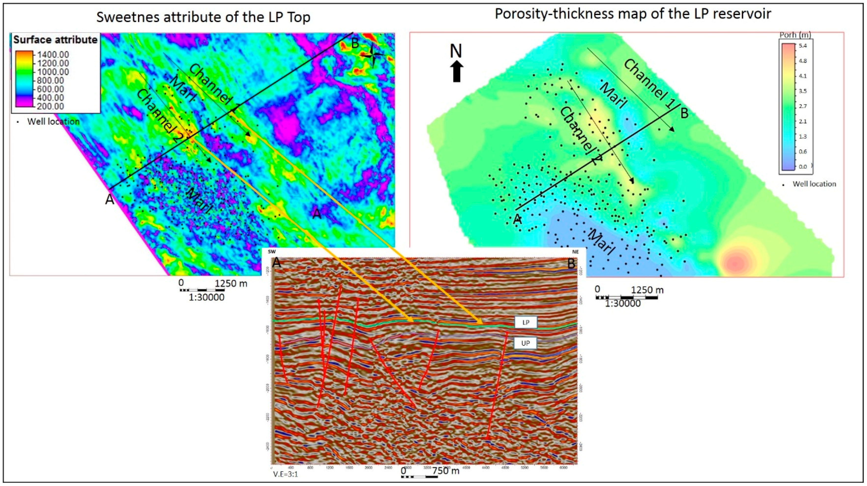
Figure 6b shows the sweetness attribute extracted parallel to the interpreted “LP” horizon in a range of 16 ms (8 ms above and 8 ms below) around the horizon. In the central part of the observed area, as mentioned above, seismic data is of poor quality but in the surrounding area, higher values of the attribute are visible in the shape of a channel-like reflection, which is associated with the sandstone distribution deposits of the “LP” reservoir.
2.2. Porosity—Thickness Maps
A geological model was constructed using PetrelTM software (Schlumberger, Houston, TX, USA). The input data set used for geological model construction for both the “UP” and “LP” reservoirs is comprised of 3D seismic interpretation for the structure definition, well log data, quantitative log analysis, core data and production data. All of this data has been integrated and analyzed in order to provide an accurate geological model. A 3D structural model enabled the construction of isochore maps. Zone is defined based on well logs data, i.e., by well to well correlation of the Spontaneous potential logs. Difference between top and bottom of the zone defined on the well logs represents zone thickness. Isochore maps were plotted by the “convert zone to isochore” option in Petrel (see Figure 7).
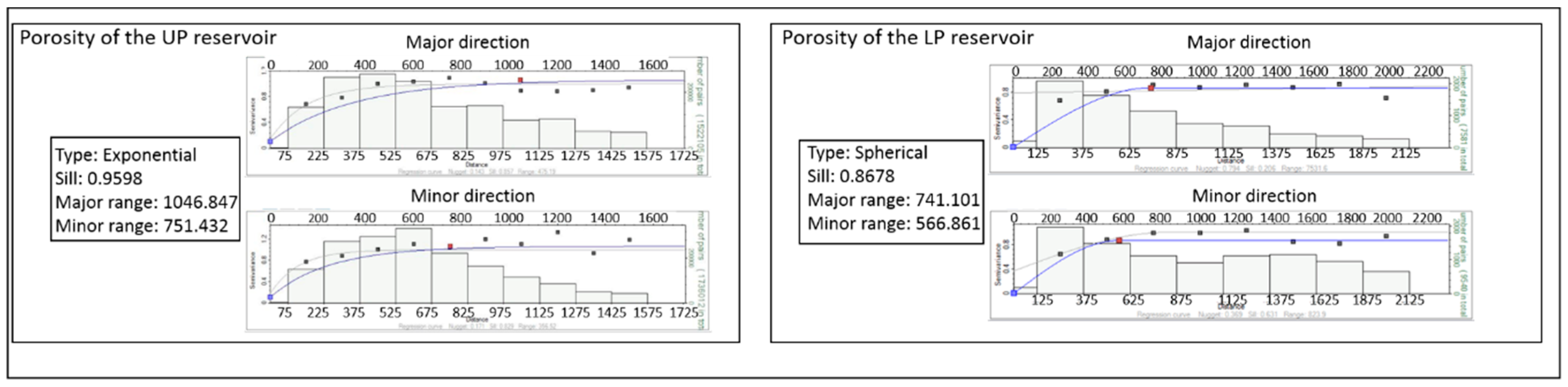
After structural model definition, a petrophysical model was defined. The analysis of petrophysical parameters was performed using the following data: (a) Quantitative log analyses of porosity, water saturations and shale volumes and (b) cored intervals–porosity measurements, khor and kver. Three sets of wells were used for the quantitative log analysis of porosity. The first set were “key wells”, which had Density–Neutron logs and cored intervals for porosity estimation. Selected wells were equally distributed through the field. The second set were wells with Neutron-Density logs, without cores. Porosity was calculated from Density–Neutron and corrected based on the first set of wells. The third set were old wells without Density–Neutron and cores. In those wells, porosity was calculated based on the Spontaneous potential log and corrected by the first two sets of wells. Log porosity was also corrected for overburden pressure, based on measurements made on the cores. The corrected porosity logs were then upscaled in the model representing input for porosity modelling. Upscaling is a process of averaging input data as a minimum, maximum or arithmetic in the model cells. In the upscaling process of the field “A” reservoirs (“UP” and “LP”), the scale-up method was an arithmetic average. Nevertheless, there are some uncertainties and errors derived from the scale-up method, i.e., if there were some thin sandy layers (thinner than the cell) with high porosity values, they would be ignored in the upscaling process and the average value at this location would be low. For porosity distribution of the “UP” and the “LP” reservoirs, variogram parameters such as model, range, sill and nugget were defined (see Figure 8).
Porosity was distributed using the deterministic ordinary kriging method, which is a mathematically advanced deterministic interpolation method for estimating variable values at the grid point [30,31]. The method is used to determine the spatial relationship between measured data and locations without any measurements where the values should be estimated. Since it uses local variance, the difference between the expected and estimated values is minimal. Geostatistical methods and their application in reservoir description are very well described in many papers [30,31,32,33,34,35,36,37,38,39,40,41]. From the distributed porosity in 3D model, average maps were created (see Figure 9).
The assumption was that both variables (porosity and thickness) can describe depositional channels, i.e., better porosities and higher thicknesses are positioned in the channel center, while lower porosities and thicknesses represent transitional lithofacies towards the basinal marls. Porosity–thickness maps were obtained by multiplying the average map of distributed porosity with isochore maps. It is clearly visible that those maps can better describe depositional channels than porosity or thickness maps separately (see Figure 10).
3. Results
Porosity–thickness maps were compared with the sweetness seismic attribute. Visually, there is a good match between them. The sweetness attribute as well as porosity–thickness maps reliably describe reservoir quality and locations of depositional channels in both the “UP” and “LP” reservoirs (see Figure 11 and Figure 12). Both of them show transported material in the general direction of NW-SE. Nevertheless, there are some differences in the mapped properties. Most of the mismatches are in areas of decreased reservoir thickness or without reservoirs, i.e., in the areas where basinal marls were deposited. It could be explained with a low resolution of seismic survey. Due to the seismic scale, seismic reflex covers a wider area, which means that the reflex could be affected with lower and deeper reservoirs. In the central part of the observed area, seismic data shows poor quality which is possibly caused by faulting or gas appearances in the shallow deposits.
It is visible especially in the areas where the observed reservoirs are very thin or absent. Therefore, it is possible to conclude that porosity–thickness maps are even better at describing depositional channels and reservoirs quality since they are a direct result of the data measured in the wells. Of course, this can apply only to areas covered with wells, but any extraction of the channels to a wider area cannot be done without seismic interpretation.
In order to prove a visual match between the sweetness seismic attribute and porosity–thickness maps, correlations between them was determined. Correlation was determined only for the “LP” reservoir. Values of the sweetness attribute at the well location, and the multiplied porosity and thickness values, also at the well locations, were normalized and compared for three cases. The first case is a comparison of all well data at the field (see Figure 13). The determination coefficient “r2” is 0.25 (correlation coefficient “r” is 0.5).
The second case represents only the north-eastern part of the reservoir where a clear depositional channel is visible (see Figure 14). This part of the reservoir is more representative than the whole reservoir in the first case because of higher thicknesses which means that the seismic attribute cannot be contaminated with deeper and lower sandstones. In this case, the general trend is much clearer and the determination coefficient “r2” is 0.42 (correlation coefficient “r” is 0.65).
The third case also represents the north-eastern part of the reservoir with a clear depositional channel, but all the noisy parts of a seismic survey are eliminated from the analysis (see Figure 15). This part of the reservoir is even more representative than the first two cases due to the high thickness of the reservoir and good seismic quality. Determination coefficient is “r2” is 0.73 (correlation coefficient “r” is 0.85).
4. Conclusions
Generally, this study proves that in case of a lack of seismic data, porosity–thickness maps, created from an abundant amount of well data, can be used to describe depositional channels of turbidity sandstones deposited during the Upper Pannonian and Lower Pontian periods in the Sava Depression. This applies only to areas covered with wells. Any extraction of a turbidity channel cannot be done without seismic data.
The analyzed reservoirs “UP” and “LP” of field “A” deposited in the Sava Depression through turbidity currents sourced from the Eastern Alps. Location of the depositional channels could be only assumed based on the average porosity or isochore maps. By multiplying them (porosity–thickness maps), depositional channels become clearly visible. The sweetness attribute and porosity–thickness maps confirm the existence of the turbidity channels and the regional material transport direction.
A comparison of the sweetness seismic attribute and porosity–thickness maps show a good visual match for both the “UP” and the “LP” reservoirs. Still, there is a mismatch, especially in areas with decreased reservoir thickness or in areas where basinal marls were deposited. The reason for that is a low resolution of seismic data. If the analyzed reservoir is thin, that interval could include deeper or shallower sandstones deposited below or above the analyzed strata. Unlike the sweetness attribute, porosity thickness maps are based on the well data. From that point of view, locations of the depositional channels and different lithofacies can be better described with porosity–thickness maps. An important condition is an abundant amount of well data, which makes a petrophysical model reliable.
Author Contributions
Conceptualization, K.N.Z. and K.N.M.; Methodology, K.N.Z.; Software, K.N.Z., S.B. and K.N.M.; Validation, K.N.M.; Formal Analysis, K.N.M.; Investigation, K.N.Z.; Resources, K.N.Z. and S.B.; Data Curation, K.N.Z. and S.B.; Writing—Original Draft Preparation, K.N.Z. and S.B.; Writing—Review and Editing, K.N.M.; Visualization, K.N.M.; Supervision, K.N.Z. and K.N.M.
Funding
Publication process is supported by the Development Fund of the Faculty of Mining, Geology and Petroleum Engineering, University of Zagreb.
Conflicts of Interest
The authors declare no conflict of interest.
References
- Taner, M.T.; Koehler, F.; Sheriff, R.E. Complex seismic trace analysis. Geophysics 1979, 44, 1041–1063. [Google Scholar] [CrossRef]
- Radovich, B.J.; Oliveros, R.B. 3D sequence interpretation of seismic instantaneous attributes from the Gorgon Field. Lead. Edge 1998, 17, 1286–1293. [Google Scholar] [CrossRef]
- Koson, S. Enhancing Geological Interpretation with Seismic Attributes in Gulf of Thailand. Master’s Thesis, Chulalongkorn University, Bangkok, Thailand, 2014. [Google Scholar]
- Alves, T.M.; Omosanya, K.; Gowling, P. Volume rendering of enigmatic high-amplitude anomalies in Southeast Brazil: A workflow to distinguish lithologic features from fluid accumulations. Interpretation 2015, 3, 1–14. [Google Scholar] [CrossRef]
- Zeng, H.; Loucks, R.; Janson, X.; Wang, G.; Xia, Y.; Yuan, B.; Xu, L. Three-dimensional seismic geomorphology and analysis of the Ordovician paleokarst drainage system in the central Tabei Uplift, northern Tarim Basin, western China. AAPG Bull. 2011, 95, 2061–2083. [Google Scholar] [CrossRef]
- Harishidayat, D.; Omosanya, K.; Johansen, S. 3D seismic interpretation of the depositional morphology of the Middle to Late Triassic fluvial system in Eastern Hammerfest Basin, Barents Sea. Mar. Petrol. Geol. 2015, 68, 470–479. [Google Scholar] [CrossRef]
- Hart, B. Channel detection in 3-D seismic data using sweetness. AAPG Bull. 2008, 92, 733–742. [Google Scholar] [CrossRef]
- Novak Zelenika, K. Deterministički i Stohastički Geološki Modeli Gornjomiocenskih Pješčenjaških Ležišta u Naftno-Plinskom Polju Kloštar. Ph.D. Thesis, Rudarsko-geološko-naftni fakultet Sveučilišta u Zagrebu, Zagreb, Croatia, 2012. [Google Scholar]
- Velić, J.; Weisser, M.; Saftić, B.; Vrbanac, B.; Ivković, Ž. Petreloleum-geological characteristics and exploration level of the three Neogene depositional megacycles in the Croatian part of the Pannonian basin. Nafta 2002, 53, 239–249. [Google Scholar]
- Ćorić, S.; Pavelić, D.; Rögl, F.; Mandic, O.; Vrabac, S.; Avanić, R.; Jerković, L.; Vranjković, A. Revised Middle Miocene datum for initial marine flooding of North Croatian Basins (Pannonian Basin System, Central Paratethys). Geol. Croat. 2009, 62, 31–43. [Google Scholar] [CrossRef]
- Malvić, T. Review of Miocene shallow marine and lacustrine depositional environments in Northern Croatia. Geol. Q. 2012, 56, 493–504. [Google Scholar] [CrossRef] [Green Version]
- Malvić, T.; Velić, J. Neogene Tectonics in Croatian Part of the Pannonian Basin and Reflectance in Hydrocarbon Accumulations. In New Frontiers in Tectonic Research: At the Midst of Plate Convergence; Schattner, U., Ed.; InTech: Rijeka, Croatia, 2011; pp. 215–238. [Google Scholar] [CrossRef]
- Horvath, F.; Tari, G. IBS Pannonian Basin Project: A review of the main results and their bearings on hydrocarbon exploration. In The Mediterranean Basins: Tertiary Extension within the Alpine Orogen; Durand, B., Jolivet, L., Horvath, F., Seranne, M., Eds.; Geological Society London: London, UK, 1999; Volume 156, pp. 195–213. [Google Scholar]
- Malvić, T. Regional turbidites and turbiditic environments developed during Neogene and Quaternary in Croatia. Mater. Geoenviron. 2016, 63, 39–54. [Google Scholar] [CrossRef] [Green Version]
- Frisch, W.; Kuhlemann, J.; Dunkl, I.; Brügel, A. A palinspastic reconstruction and topographic evolution of the Eastern Alps during the Tertiary tectonical evolution. Tectonophysics 1998, 297, 1–15. [Google Scholar] [CrossRef]
- Vrbanac, B. Paleostrukturne i sedimentološke analize gornjopanonskih naslaga formacije Ivanić-Grad u Savskoj depresiji. Ph.D. Thesis, Prirodoslovno.-matematički. fakultet Sveučilišta. u Zagrebu, Zagreb, Croatia, 1996. [Google Scholar]
- Rögl, F. Stratigraphic Correlation of the Paratethys Oligocene and Miocene. Mitteilungen Ges. Geol. Bergbaustudenten Österreich 1996, 41, 65–73. [Google Scholar]
- Rögl, F. Palaeographic Consideration for Mediterranean and Paratethys Seaways (Oligocene to Miocene). Ann. Naturhist. Mus. Wien 1998, 99A, 279–310. [Google Scholar]
- Malvić, T. Middle Miocene Depositional Model in the Drava Depression Described by geostatistical porosity and thickness maps (case study: Stari Gradac-Barcs Nyugat Field). Min. Geol. Petrol. Bull. 2006, 18, 63–70. [Google Scholar]
- Royden, L.H. Late Cenozoic Tectonics of the Pannonian Basin System. In The Pannonian Basin; Royden, L.H., Horváth, F., Eds.; AAPG Memoir: Tulsa, OK, USA, 1988; Volume 45, pp. 27–48. ISBN 0891813225. [Google Scholar]
- Malvić, T.; Velić, J.; Peh, Z. Qualitative-Quantitative Analyses of the Influence of Depth and Lithological Composition on Lower Pontian Sandstone Porosity in the Central Part of Bjelovar Sag (Croatia). Geol. Croat. 2005, 58, 73–85. [Google Scholar]
- Vrbanac, B.; Velić, J.; Malvić, T. Sedimentation of deep-water turbidites in main and marginal basins in the SW part of the Pannonian Basin. Geol. Carpath. 2010, 61, 55–69. [Google Scholar] [CrossRef]
- Rögl, F.; Steininger, F.; Neogene Paratethys, C.; Brenchey, P.J. (Eds.) Geological Journal, Special Issue; Wiley and Sons: Chichester, UK, 1984; Volume 11, pp. 171–200. ISBN 047190418X. [Google Scholar]
- Saftić, B.; Velić, J.; Sztano, O.; Juhas, G.; Ivković, Ž. Tertiary subsurface facies, source rocks and hydrocarbon reservoirs in the SW part of the Pannonian Basin (northern Croatia and south-western Hungary). Geol. Croat. 2003, 56, 101–122. [Google Scholar]
- Šimon, J. Prilog stratigrafiji u taložnom sustavu pješčanih rezervoara Sava-grupe naslaga mlađeg tercijara u Panonskom bazenu sjeverne Hrvatske. Ph.D. Thesis, Rudarsko-geološko-naftni fakultet Sveučilišta u Zagrebu, Zagreb, Croatia, 1980. [Google Scholar]
- Šimon, J. Prilog stratigrafskoj analizi tercijarnih sedimenata na sjeverozapadnom predjelu Savske potoline. In Proceedings of the VII kongres geologa Socijalističke Federativne Republike Jugoslavije, Zagreb, Croatia, 1970; pp. 347–360. [Google Scholar]
- Šimon, J. O nekim rezultatima regionalne korelacije litostratigrafskih jedinica u jugozapadnom području Panonskog bazena. Nafta 1973, 24, 623–630. [Google Scholar]
- Novak Zelenika, K.; Velić, J.; Malvić, T. Local sediment sources and palaeoflow directions in Upper Miocene turbidites of the Pannonian Basin System (Croatian part), based on mapping of reservoir properties. Geol. Q. 2013, 57, 17–30. [Google Scholar] [CrossRef]
- Novak Zelenika, K.; Smoljanović, S. Correction of the seismic attribute sweetness by using porosity-thickness map, Lower Pontian LP reservoir, Sava Depression. In Mathematical Methods and Terminology in Geology; Malvić, T., Velić, J., Rajić, R., Eds.; Rudarsko-geološko-naftni fakultet Sveučilišta u Zagrebu: Zagreb, Croatia, 2018; pp. 77–86. [Google Scholar]
- Krige, D.G. A statistical approach to some basic mine valuation problems on the Witwatersrand. J. Chem. Metall. Min. Soc. S. Afr. 1951, 52, 119–139. [Google Scholar]
- Matheron, G. Les Variables Regionalisees et Leur Estimation: Une Application de la Theorie des Functions Aleatoires Aux Sciences de la Mature; Masson: Paris, France, 1965; p. 306. [Google Scholar]
- De Wijs, H.J. Statistics of ore distribution. Part I: Frequency distribution of assay values. J. Royal Neth. Geol. Min. Soc. 1951, 13, 365–375. [Google Scholar]
- Hohn, M.E. Geostatistics and Petroleum Geology; Van Nostrand Reinhold: New York, NY, USA, 1988; p. 264. [Google Scholar]
- Isaaks, E.; Srivastava, R. An Introduction to Applied Geostatistics; Oxford University Press Inc.: New York, NY, USA, 1989; p. 580. [Google Scholar]
- Cai, Z.; Hicks, P.J., Jr. 3D conditional simulation of porosity for a heterogeneous core. J. Can. Petrol. Technol. 1999, 38, 46–52. [Google Scholar] [CrossRef]
- Dubruble, O. Geostatistics in Petroleum Geology; AAPG Education Course Note, Series #38; AAPG and Geological Society Publishing House: Tulsa, OK, USA, 1998; p. 210. [Google Scholar]
- Malvić, T.; Jović, G. Thickness maps of Neogene and Quaternary sediments in the Kloštar Field (Sava Depression, Croatia). J. Maps 2012, 8, 260–266. [Google Scholar] [CrossRef] [Green Version]
- Novak Zelenika, K.; Cvetković, M.; Malvić, T.; Velić, J.; Sremac, J. Sequential indicator simulations maps of porosity, depth and thickness of Miocene clastic sediments in the Kloštar Field, Northern Croatia. J. Maps 2013, 9, 550–557. [Google Scholar] [CrossRef]
- Malvić, T.; Novak, K.; Novak Zelenika, K. Indicator Kriging porosity maps of Upper Miocene sandstones, Sava Depression, Northern Croatia. RMZ Mater. Geookolje 2015, 62, 37–45. [Google Scholar]
- Novak Zelenika, K. Theory of deterministical and stochastical indicator mapping methods and their applications in reservoir characterization, case study of the Upper Miocene reservoir in the Sava Depression. Min. Geol. Petrol. Bull. 2017, 32, 45–53. [Google Scholar] [CrossRef]
- Al-Mudhafar, W.J. How is multiple-point geostatistics of lithofacies modeling assisting for fast history matching? A case study from a sand-rich fluvial depositional environment of Zubair formation in South Rumaila Oil Field. In Proceedings of the Offshore Technology Conference, Huston, TX, USA, 30 April 2018. [Google Scholar] [CrossRef]
Figure 1.
Stratigraphic column, megacycles, environments, tectonic phases and lithology in the Sava Depression [28].
Figure 1.
Stratigraphic column, megacycles, environments, tectonic phases and lithology in the Sava Depression [28].

Figure 2.
Location of the analyzed area [22].
Figure 2.
Location of the analyzed area [22].

Figure 3.
General chronostratigraphy–lithofacies column of field “A”.

Figure 4.
Flowchart of applied methodology.

Figure 5.
Seismic section of the mapped horizons (a) “UP” (Upper Pannonian) reservoir and (b) “LP” (Lower Pontian) reservoir.
Figure 5.
Seismic section of the mapped horizons (a) “UP” (Upper Pannonian) reservoir and (b) “LP” (Lower Pontian) reservoir.

Figure 6.
Sweetness attribute showing (a) an interval of 4 ms above and 4 ms below “UP” horizon and (b) an interval of 8 ms above and 8 ms below “LP” horizon [29].
Figure 6.
Sweetness attribute showing (a) an interval of 4 ms above and 4 ms below “UP” horizon and (b) an interval of 8 ms above and 8 ms below “LP” horizon [29].

Figure 7.
Isochore map of the (a) “UP” reservoir and (b) “LP” reservoir.

Figure 8.
Variograms of the porosity of the “UP” and “LP” reservoirs.

Figure 9.
Porosity map of the (a) “UP” reservoir and (b) “LP” reservoir.

Figure 10.
Porosity–thickness map of the (a) “UP” reservoir and (b) “LP” reservoir [29].
Figure 10.
Porosity–thickness map of the (a) “UP” reservoir and (b) “LP” reservoir [29].

Figure 11.
Comparison of the sweetness attribute and porosity–thickness map of the “UP” reservoir.

Figure 12.
Comparison of the sweetness attribute and porosity–thickness map of the “LP” reservoir [29].
Figure 12.
Comparison of the sweetness attribute and porosity–thickness map of the “LP” reservoir [29].

Figure 13.
Correlation of the sweetness attribute and porosity–thickness map of the “LP” reservoir [29].
Figure 13.
Correlation of the sweetness attribute and porosity–thickness map of the “LP” reservoir [29].

Figure 14.
Correlation of the sweetness attribute and porosity–thickness map of the north-eastern part (NE part) of the “LP” reservoir [29].
Figure 14.
Correlation of the sweetness attribute and porosity–thickness map of the north-eastern part (NE part) of the “LP” reservoir [29].

Figure 15.
Correlation of the sweetness attribute and porosity–thickness map of the best part of the “LP” reservoir with clear seismic survey measurements.
Figure 15.
Correlation of the sweetness attribute and porosity–thickness map of the best part of the “LP” reservoir with clear seismic survey measurements.

© 2018 by the authors. Licensee MDPI, Basel, Switzerland. This article is an open access article distributed under the terms and conditions of the Creative Commons Attribution (CC BY) license (http://creativecommons.org/licenses/by/4.0/).
Share and Cite
MDPI and ACS Style
Novak Zelenika, K.; Novak Mavar, K.; Brnada, S. Comparison of the Sweetness Seismic Attribute and Porosity–Thickness Maps, Sava Depression, Croatia. Geosciences 2018, 8, 426. https://doi.org/10.3390/geosciences8110426
AMA Style
Novak Zelenika K, Novak Mavar K, Brnada S. Comparison of the Sweetness Seismic Attribute and Porosity–Thickness Maps, Sava Depression, Croatia. Geosciences. 2018; 8(11):426. https://doi.org/10.3390/geosciences8110426
Chicago/Turabian StyleNovak Zelenika, Kristina, Karolina Novak Mavar, and Stipica Brnada. 2018. "Comparison of the Sweetness Seismic Attribute and Porosity–Thickness Maps, Sava Depression, Croatia" Geosciences 8, no. 11: 426. https://doi.org/10.3390/geosciences8110426
Note that from the first issue of 2016, this journal uses article numbers instead of page numbers. See further details here.