Assessment of Earth Gravity Field Models in the Medium to High Frequency Spectrum Based on GRACE and GOCE Dynamic Orbit Analysis


1
Geoscience Australia, Cnr Jerrabomberra Ave and Hindmarsh Drive, Symonston, ACT 2609, Australia
2
Cooperative Research Centre for Spatial Information, Docklands, VIC 3008, Australia
3
Department of Geodesy and Surveying, Aristotle University of Thessaloniki, 54124 Thessaloniki, Greece
*
Author to whom correspondence should be addressed.
Geosciences 2018, 8(12), 441; https://doi.org/10.3390/geosciences8120441
Submission received: 22 October 2018
/
Revised: 19 November 2018
/
Accepted: 23 November 2018
/
Published: 27 November 2018
(This article belongs to the Special Issue Gravity Field Determination and Its Temporal Variation)
Abstract
:An analysis of current static and time-variable gravity field models is presented focusing on the medium to high frequencies of the geopotential as expressed by the spherical harmonic coefficients. A validation scheme of the gravity field models is implemented based on dynamic orbit determination that is applied in a degree-wise cumulative sense of the individual spherical harmonics. The approach is applied to real data of the Gravity Field and Steady-State Ocean Circulation (GOCE) and Gravity Recovery and Climate Experiment (GRACE) satellite missions, as well as to GRACE inter-satellite K-band ranging (KBR) data. Since the proposed scheme aims at capturing gravitational discrepancies, we consider a few deterministic empirical parameters in order to avoid absorbing part of the gravity signal that may be included in the monitored orbit residuals. The present contribution aims at a band-limited analysis for identifying characteristic degree ranges and thresholds of the various GRACE- and GOCE-based gravity field models. The degree range 100–180 is investigated based on the degree-wise cumulative approach. The identified degree thresholds have values of 130 and 160 based on the GRACE KBR data and the GOCE orbit analysis, respectively.
1. Introduction
Orbit determination is a core topic in satellite geodesy, comprising both geometrical and dynamical aspects in the pursuit of constructing a detailed mathematical model that can describe the motion of an artificial satellite orbiting Earth as accurately as possible [1]. The link between the geometric form of the evolving orbit and the underlying Earth’s gravity field has been the subject of extensive scientific elaboration that spans a time period coinciding with the satellite era itself. Mathematical rigor and computational efficiency, especially in the dawn of direct satellite observations of ever growing magnitude and accuracy, have been the main pillars of these contributions that include numerical, analytical or hybrid approaches [2,3,4,5,6,7,8,9,10,11]. With the advent of a vast number of new satellite-only and combined gravity field models, the main bulk of which are routinely produced from the analysis of currently available satellite data, the problem of orbit determination, especially its dynamic counterpart, received an abundance of solutions for the numerical computation of Earth’s gravitational attraction at satellite altitude. The scope of the present contribution is to expose the role of an individual selection of a global solution to Earth’s gravity field, given in terms of a finite number of potential harmonic coefficients, to the computation of the pure gravitational component in the satellite’s equation of motion. It is not our primary goal to present or pursue a closed loop of a dynamic orbit determination procedure of the highest possible level of accuracy. Rather, we intend to establish a validation mechanism for an in-orbit assessment and analysis of the different gravity field models, when their contribution is considered in a coefficient-wise manner. By switching again from potential to geometry through an expression of the aforementioned contributions in the orbital frame as position disturbances along the three axes, one is able to quantify the information content of any gravity field model, both as a global solution as well as in a band-limited fashion. With the proposed scheme, an additional insight to the computation of the equation of motion is envisaged, while at the same time an independent possibility is offered to model and validate highly precise satellite data, such as Gravity Recovery and Climate Experiment (GRACE)-like inter-satellite ranges and range rates.
During the last two decades, gravity field determination has been based on the innovative concepts introduced by satellite missions dedicated for the gravity field mapping (i.e., CHAllenging Mini-satellite Payload (CHAMP), Gravity Recovery and Climate Experiment (GRACE) and Gravity field and steady-state Ocean Circulation Explorer (GOCE) satellite missions [12,13,14,15]. The three satellite missions are no longer in orbit and the operational dates were 15 July 2000–19 September 2010 for CHAMP, 17 March 2002–27 October 2017 for GRACE, and 17 March 2009–21 October 2013 for GOCE. The space-borne observation techniques introduced by these satellite gravity missions have generated the numerical investigation of various methods in gravity field modeling and a numerous series of satellite gravity field models has been produced based on various methods [16,17,18]. The gravity field models are available free of charge from the International Centre for Global Earth Models (ICGEM) web page [19].
Furthermore, time-variable gravity field models have been demonstrated during the last decade based on the GRACE mission [20,21]. The monitoring of time-variations series of the gravity field is a topic of high interest in the frame of the past and future satellite gravity missions [22,23,24] such as the Gravity Recovery and Climate Experiment-Follow-On (GRACE-FO) mission [25], which was recently launched on 22 May 2018.
The validation of gravity field models, as determined by various approaches, into the overall frequency spectrum of the gravity field is a critical aspect for satellite gravity missions’ performance and for any further studies regarding Earth’s interior based on the adopted gravity field models [18,26,27,28,29]. The present study presents a frequency analysis of current time-variable and static gravity field models, focusing on the medium to high frequencies of the geopotential as represented by the degree range 100 to 200 in terms of spherical harmonics. The validation scheme of the gravity field models is implemented here based on a dynamic orbit determination algorithm that is applied in a degree-wise cumulative sense of the individual spherical harmonics. The orbit determination is repeated as a function of the geopotential truncation degree and we monitor the respective orbit residuals in order to obtain an insight to the spectral content of the gravity field models. The specific degree range has been selected based on the sensitivity of the applied orbit determination scheme. The discrepancies of the orbit and KBR residuals are becoming smooth for degrees higher than 200.
The proposed approach is applied to real GRACE and GOCE data. We focus on the analysis of the GRACE KBR data. Due to the high accuracy of KBR data, at the level of a few μm, such an approach defines an external validation tool of the gravity field models. The present contribution aims at a band-limited analysis for identifying characteristic degree ranges and thresholds of the various GRACE- and GOCE-based gravity field models.
2. Dynamic Orbit Determination
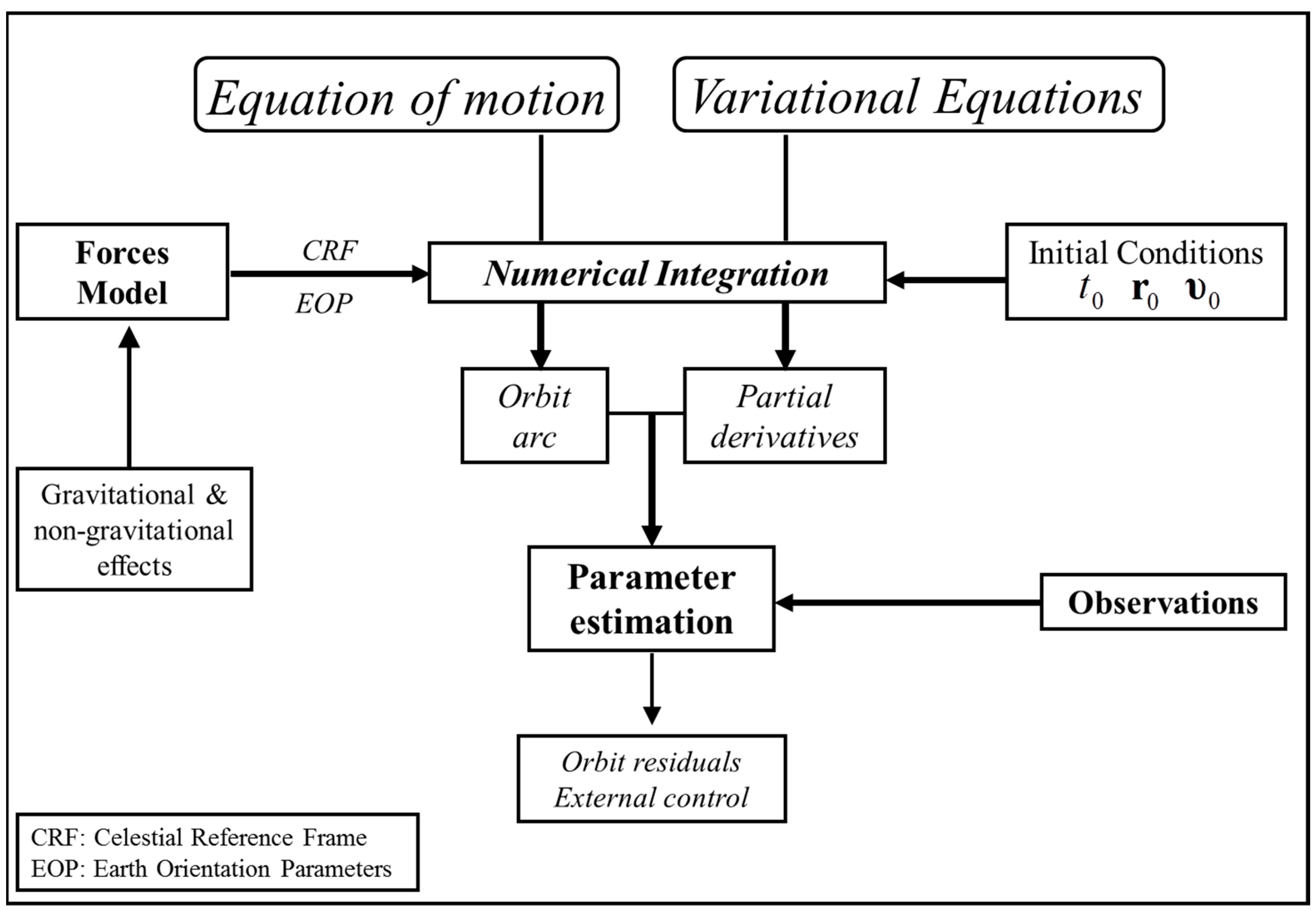
The principal objectives included in satellite orbit determination are given in Figure 1 as presented by [30].
The present orbit analysis follows this approach of dynamic orbit determination focusing on the effects of Earth’s gravity field. In particular, the equations system of orbit determination is consists of the equation of motion and its partial derivatives, the so-called variational equations. The equation of motion is expressed through Newton’s second law that forms the basic mathematical tool for describing a satellite orbit:
where denotes the acceleration vector, m the satellite’s mass and the sum of all forces acting on the satellite, which in general includes both gravitational and non-gravitational contributions.
The solution of the equations system is achieved through numerical integration methods suitable for ordinary differential equations [32,33]. The performance of the numerical integration methods is critical and depends on the integration step and the method’s order. The impact of the numerical integrators in dynamic orbit determination has been extensively investigated in a previous study [34]. In the current analysis, we apply the Gauss–Jackson numerical integration method that solves directly 2nd order differential equations. The equation of motion and the variational equations have to be integrated simultaneously and the numerical solution provides the orbital arc and the partial derivatives of the parameters of interest to be estimated. The solution of this system of differential equations along with the satellite observations are used in the orbit parameter estimation method. Our approach of the overall solution is summarized by the following algorithm of five steps:
- Simultaneous numerical integration of the variational equations and the equation of motion is performed based on a simplified force model. In the present analysis, we consider only the gravity field model, truncated to degree and order of 50. The effects of the empirical parameters are also included at this step.
- The design matrix of the estimator is formed based on the solution of the variations equations.
- Numerical integration of the equation of motion is applied based on the full force model as summarized in Table 1.
- The observation equations are formed based on the numerical solution of the previous step.
- The parameter estimation is then applied. One or two iterations steps may be required.
Following the aforementioned steps, the orbit parameter estimator is applied considering the least-squares method and the use of pseudo-observations [16,41] based on available a priori orbits such as kinematic orbit data [42]. One iteration step was found to be sufficient in terms of orbit residuals improvement. The observation equations based on pseudo-observations are formulated by the differences of the satellite position vector
where , , are the Cartesian coordinates as provided by the kinematic orbit data and express the observation errors. , , refer to the satellite position vector obtained by the orbit integration (numerical solution of the equation of motion).
In the present analysis, the estimated parameters include the initial position and velocity vector of the satellite and additional force-related parameters. The additional parameters refer to empirical accelerations such as bias and cycle per revolution accelerations [43,44]. We have considered a minimum number of empirical accelerations in order to avoid absorbing residuals that may include part of the gravity signal [45,46].
2.1. Degree-Wise Cumulative Approach
A basic tool for the synthetic evaluation of Earth’s gravity field functionals is the expression of the gravitational potential V in terms of a spherical harmonic expansion [47]
where GM is the product between the gravitational constant G and Earth’s total mass M, is the equatorial radius, (r, θ, λ) are the spherical coordinates of the satellite’s position, and are the normalized spherical harmonic coefficients of a given gravity field model and are the normalized associated Legendre functions, with n and m denoting degree and order, respectively.
The expansion series of Equation (2), as well as its partial derivatives that lead to gravitational constituents, are treated here in a degree-wise cumulative sense. We repeat the orbit estimation procedure for each degree and the geopotential expansion series is formed by using all previous harmonic coefficients up to that specific degree, with the rest of the orbit parameters left unchanged. This approach can reveal the dynamic contribution of the coefficients belonging to an individual degree at satellite altitude.
2.2. Orbit Resonances and Order-Wise Analysis
The dynamic orbit analysis based on the aforementioned degree-wise cumulative approach, may be affected by resonance effects [2]. Orbit resonances may occur in the case of artificial satellites [2,49] and affect the specific order of the spherical harmonic coefficients that represent the gravity field based on Equation (3), the so called lumped coefficients [2,50]. The investigation of resonance effects in gravity field modelling based on satellite orbits has been described by [51,52]. The impact of orbit resonances in satellite gravity missions has also been a critical topic in the design of such missions [50,53,54].
In the present analysis, we apply an order-wise cumulative approach in the GOCE orbit and GRACE KBR analysis. In particular, the degree of the spherical harmonics expansion is set to a fixed value of 180, while the order varies within the range of 2 to 180. The orbit determination is repeated for each value of the order by using all previous harmonic coefficients up to that specific order. Such an order-wise analysis aims to quantify the impact of resonance effects in the current study and to reveal potential affected harmonics coefficients.
3. GRACE and GOCE Orbit Analysis
The dynamic orbit determination concept as presented here has been applied in the cases of GRACE and GOCE satellite missions. The present contribution provides a frequency analysis, in terms of a degree-wise cumulative orbit analysis, of time-variable and static gravity field models in the range of medium to high frequencies, that is, the degree range from 100 to 200. The current analysis focuses on GRACE KBR data analysis as an assessment tool of the gravity field models. The concept of the low–low satellite-to-satellite tracking was implemented by the GRACE mission through an on-board microwave ranging system. The GRACE KBR observations may reach accuracies at the level of a few μm [55,56,57] and therefore, the KBR data analysis offers an external validation tool of the GRACE satellites orbits along the line-of-sight direction [41]. We incorporate the gravity field models into the GRACE orbit determination through the degree-wise cumulative approach and then we monitor the KBR data residuals. Based on the high accuracy of the inter-satellite ranging data, this approach forms a rigorous validation of the gravity field models applied in the orbit determination.
In particular, the GOCO05s [21,58], EIGEN-6S4 [59] and ITSG-Grace2014k [60] time-variable gravity field models have been analyzed in the present study. These time-variable gravity field models include variations of the spherical harmonic coefficients such as trends and annual terms (GOCO05s, ITSG-Grace2014k) and even semi-annual terms in the case of EIGEN-6S4 model. In addition, three static gravity field models, that is, GGM05G [61], GOCE-DIR R4 and R5 [62] have been applied in the current approach. The applied gravity field models are satellite-only models and details of their features are summarized in Table 2.
Our source code has been developed by [31] and has been used in orbit analysis by [34,41]. The current version follows the orbit modelling summarized in Table 1 and incorporates the gravity field models presented in Table 2. The performed computations consider the Matlab double precision (64 bits) floating point numerical representation. The computation time (CPU) of the orbit determination of daily orbit arcs varies from 60 to 80 min on a HP-Z400 Workstation (Intel Xeon 3.2 GHz).
3.1. Data Preprocessing
Satellite data from the GRACE and GOCE missions require a suitable preprocessing prior to further analysis in the frame of the adopted dynamic orbit determination. GRACE and GOCE data processing follows standard procedures [63,64] and details regarding data preprocessing, as implemented here, are given by [41].
In the case of GRACE, accelerometry data are considered for capturing non-gravitational effects. Precise calibration parameters of the GRACE accelerometry data are provided by the TU Delft thermosphere web server (thermosphere.tudelft.nl) [65,66].
The GRACE inter-satellite ranging data are not used as observations in the orbit estimation procedure and perform a relative control of the orbit accuracy. One critical parameter in KBR data analysis is the estimation of the unknown bias that is a characteristic of the range data. An alternative approach is also utilized which leads to the elimination of the KBR bias by forming range data differences between sequential epochs.
3.2. Empirical Parameters
Since the proposed scheme aims at capturing gravitational discrepancies, we consider a few deterministic empirical parameters in order to avoid absorbing part of the gravity signal that may be included in the monitored orbit residuals as discussed by [45,46]. In particular, bias and one cycle per revolution accelerations [43] are estimated within the orbit determination procedure. Based on the orbit residuals monitoring, the one cycle per revolution (CPR) accelerations are the dominant effect in comparison with two cycle per revolution or even higher terms. The empirical accelerations are included here in order to capture the mismodelling of the accelerometry calibration and the remaining drag-free system residuals in the case of GRACE and GOCE, respectively. The empirical parameters of the bias and once per revolution accelerations are estimated only for the along-track and cross-track components, since these directions are strongly affected by mismodelling in the non-gravitational effects.
3.3. Results
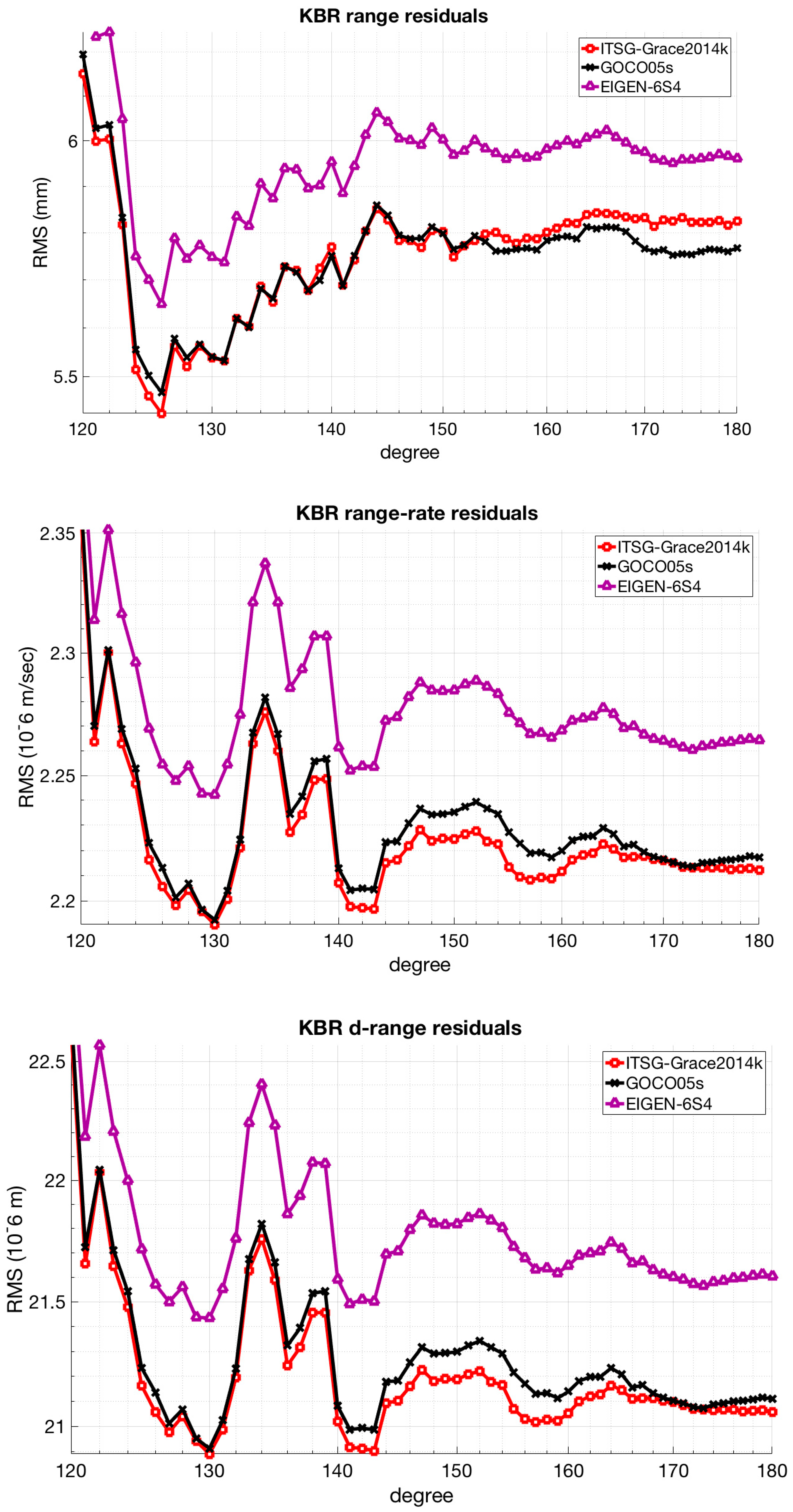
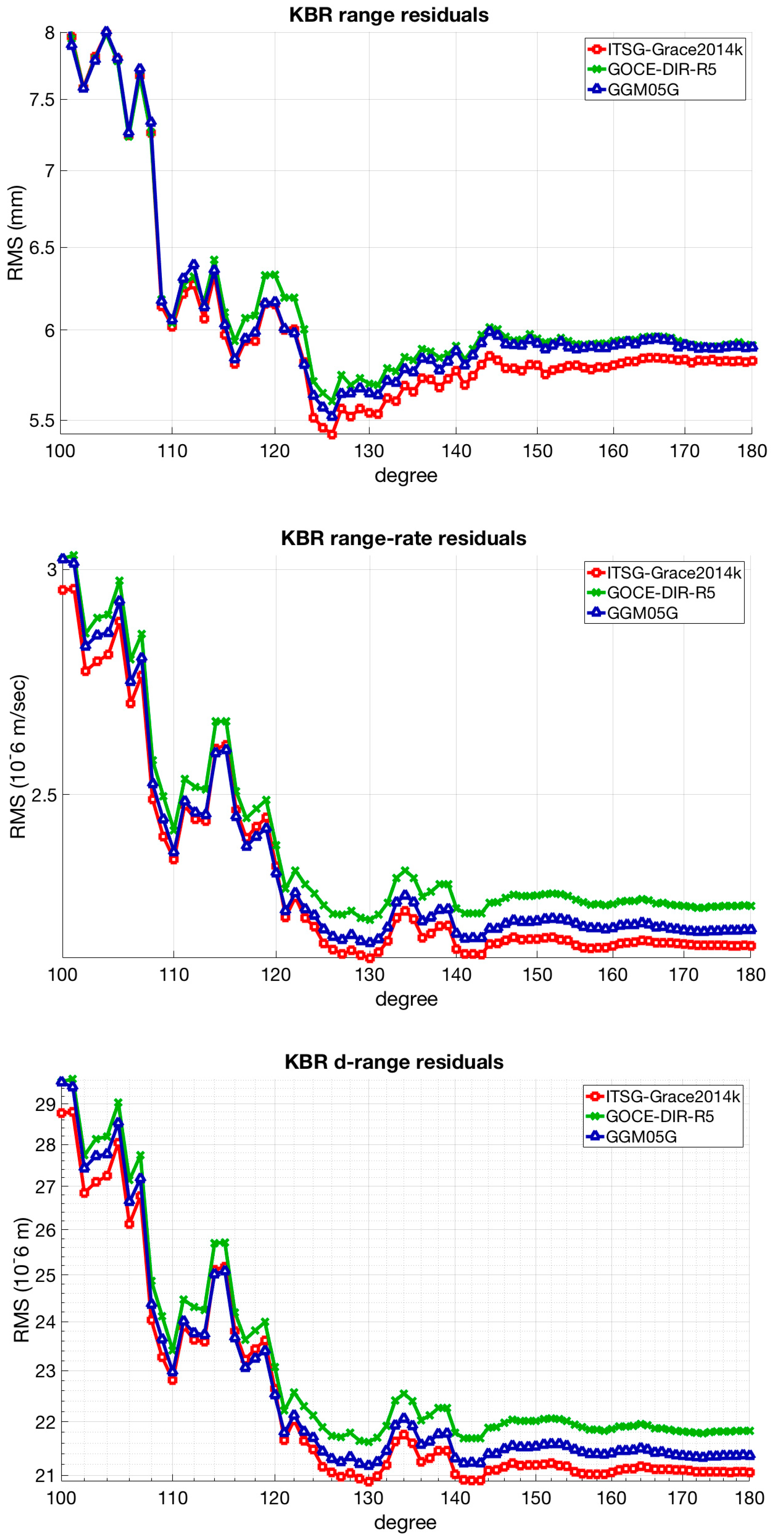
The results of the GRACE inter-satellite ranging data analysis based on the approach described here are given in Figure 2 and Figure 3 for the time-variable and static gravity field models, respectively.
In addition, the GRACE orbit and KBR residuals are provided in Table 3 and Table 4 for selected degrees of the used gravity field models. The root mean square (RMS) variations refer to the inter-satellite ranging data residuals to the range obtained by the GRACE estimated dynamic orbits.
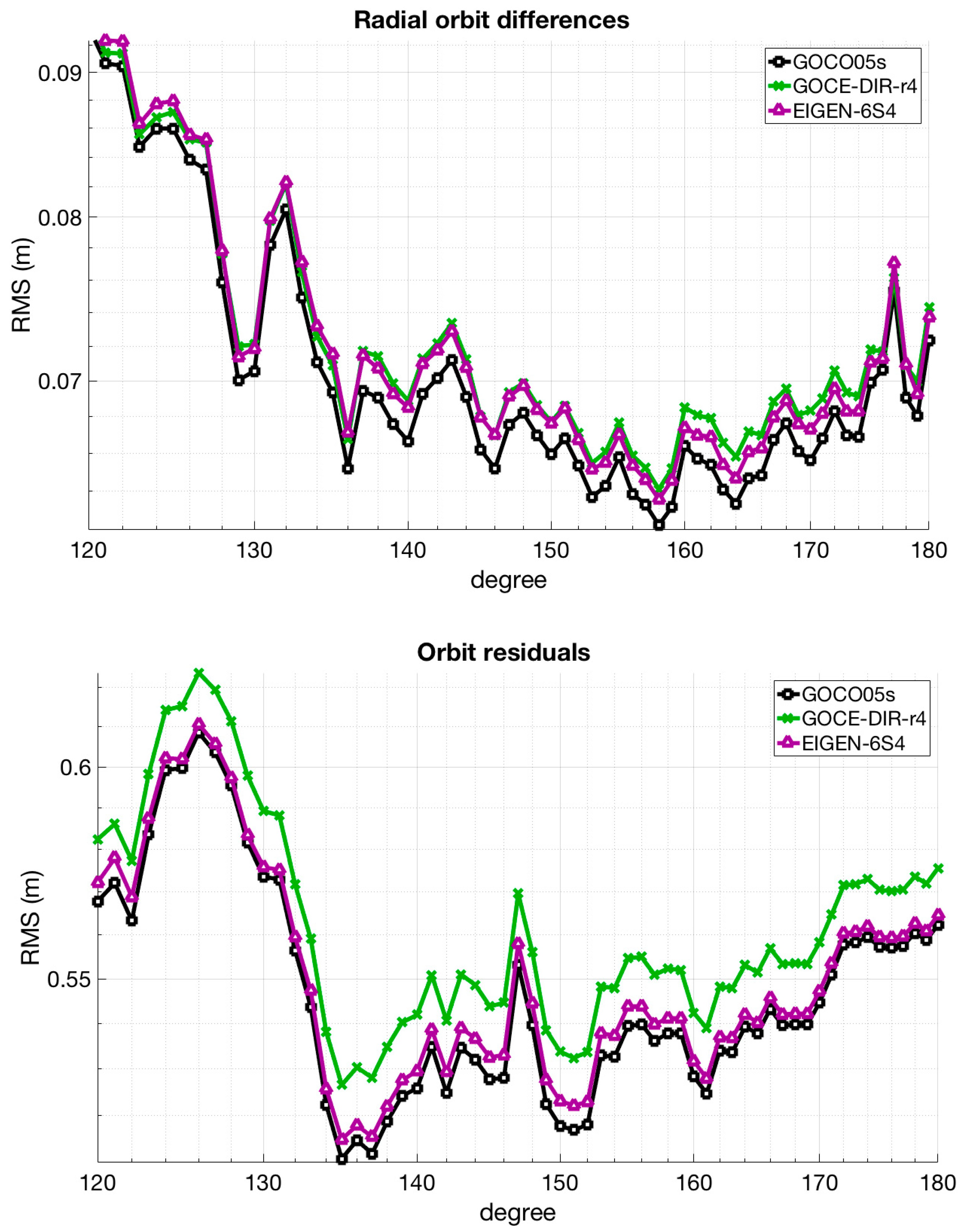
In the case of the GOCE orbit analysis, results are presented in Figure 4 and Table 5. The orbit residuals are illustrated as a function of the truncated degree of the gravity field models. In addition, the RMS variations of the numerical comparison between the GOCE estimated orbits and the reduced-dynamic precise orbit data [38] are presented in the orbital frame. In particular, we focus on the radial direction, as shown in Figure 4, since the radial component is dominated by the gravity field forces in comparison with the along-track and cross-track components. Thus, empirical parameters are not being estimated in the radial component. The mismodelling of the non-gravitational effects has an impact along the orbit motion that mostly affects the along-track direction followed by the cross-track direction. However, it should also be stated that such mismodelling could have a minor impact on the radial component.
3.4. Order Wise Analysis
In addition, the order-wise cumulative approach is applied in the dynamic orbit determination as described in Section 2.2. The order-wise orbit analysis aims to show the impact of resonance effects on the current orbit determination scheme. In particular, the degree has been fixed to 180 while the order is varying within the range of 2 to 180. The orbit determination is repeated by modifying the order value by 1 and considering all the previous harmonic coefficients up to the selected degree and order.
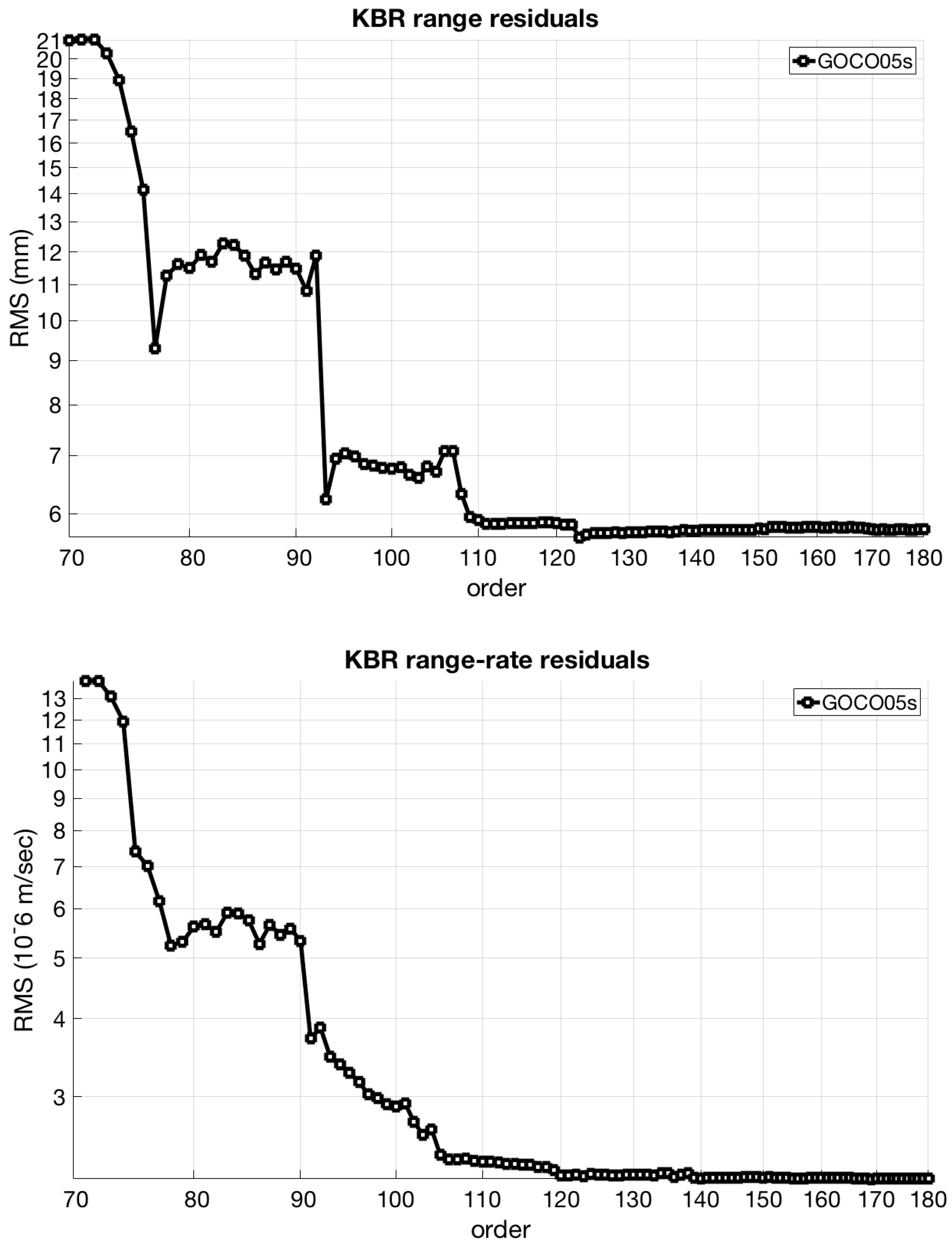
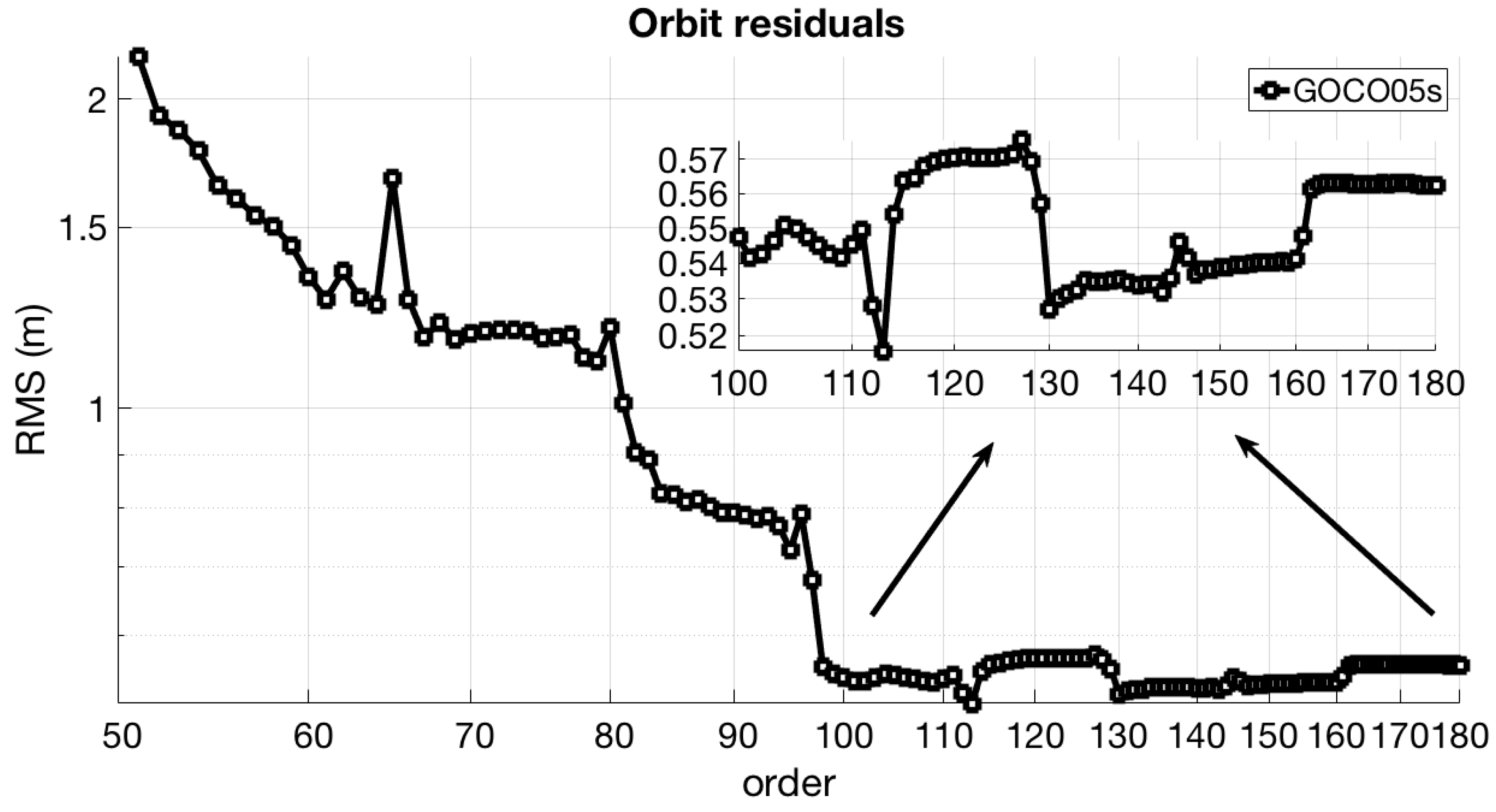
The order-wise approach has been applied for GRACE and GOCE satellites based on the GOCO05s model. The results of the GRACE inter-satellite ranging residuals are presented in Figure 5 while the GOCE orbit residuals variations are shown in Figure 6.
The order-wise analysis reveals discrepancies of a few mm in the range of 70 to 90 degrees based on the GRACE KBR range residuals, while the GOCE orbit residuals show variations at cm level within the range of 110 to 130 degrees. It should be mentioned that the resonances effects may be absorbed by the empirical parameters, that is, bias and cycle per revolution accelerations (Section 3.2) that are estimated within the dynamic orbit determination. Therefore, the variations are smooth, especially for the higher order values.
4. Discussion
The current study provides an assessment of gravity field models and presents a relative validation between them. The present analysis is based on a pure dynamic orbit determination by adding a few empirical parameters for the force mismodelling.
In the case of the GRACE mission, we focus on the inter-satellite ranging data analysis. This space-borne observation technique offers a relative validation tool along the line of sight direction. Based on the adapted orbit modeling here, the degree-wise cumulative approach captures discrepancies at the mm level, as presented in Figure 2 and Figure 3. The time-variable gravity field models lead to lower residuals in comparison with the static gravity field models. This is strongly pronounced within the overall degree range (100–180) as shown in Figure 3. In particular, the GOCO05s and the ITSG-Grace2014k models lead to equivalent performance providing the best results in terms of KBR data residuals. A threshold has been identified for degrees approaching values from 125 to 130. The KBR residuals are significantly reduced within this range while degrees higher than 150 lead to smooth variations.
In general, orbit analysis of Low Earth Orbiters (LEOs) offers a measure of the gravity field model’s performance as expressed through the orbit residuals of the gravity field model used within the orbit determination. In the present study, GOCE orbit analysis is applied as an additional tool for the assessment of gravity field models. Due to the low orbital altitude (255–229 km) of the GOCE satellite mission, GOCE orbit has higher sensitivity to the medium-high degree geopotential coefficients in comparison with other LEOs.
The GOCE orbit analysis based on the degree-wise cumulative approach leads to a similar conclusion regarding the performance of the time-variable gravity field models in comparison with the static models as presented in Figure 4. The GOCO05s model provides the lowest residuals within the overall degree range (100–180). The GOCE orbit analysis reveals that degree harmonics higher than 160 lead to increased orbit residuals. It should be mentioned that a drag-free orbit is assumed due to the existence of the GOCE drag-free control system. The remaining residuals due to the drag-free errors are modelled through the estimation of empirical parameters, that is, bias and one cycle per revolution accelerations in the along-track and cross-track directions. However, a part of the drag-free orbit errors may affect the observation residuals. Moreover, orbit resonances that may occur at specific degrees could also affect the orbit residuals.
In principle, the orbit accuracy may increase in terms of orbit residuals by estimating several additional empirical parameters. On the other hand, such a number of estimated parameters may absorb part of the gravity signal. Since we focus on the assessment of the gravity field models and the relative discrepancies in a frequency-wise sense, we apply a scheme of pure dynamic orbit determination. The degree-wise cumulative approach, based on the estimated dynamic orbits, aims at identifying specific bandwidths of the gravity field models such as the aforementioned range for degrees higher than 130 and 160 for GRACE and GOCE, respectively. In the context of our ongoing work, we should mention that further investigation is required within the identified bandwidth based on different orbit modeling and longer time periods.
Author Contributions
Methodology, T.D.P. and D.T.; Software T.D.P.; Writing—review & editing, T.D.P. and D.T.
Funding
This research received no external funding.
Acknowledgments
The authors acknowledge the European Space Agency for providing the GOCE data, GFZ for providing the GRACE data, the International Centre for Global Earth Models (ICGEM) for providing the gravity field models, the Earth Orientation Center for providing the EOP data, JPL for providing the DE data, IAU for providing the SOFA software for the precession-nutation model and DEOS at TU Delft for providing the GRACE accelerometry calibration parameters.
Conflicts of Interest
The authors declare no conflict of interest.
References
- Beutler, G. Methods of Celestial Mechanics; Springer: Berlin, Germany, 2005; Volumes I & II. [Google Scholar]
- Kaula, W.M. Theory of Satellite Geodesy; Dover Publications: New York, NY, USA, 1966. [Google Scholar]
- Rosborough, G.W. Satellite Orbit Peturbations due to the Geopotential, Center for Space Research; Report CSR-86-1; University of Texas at Austin: Austin, TX, USA, 1986. [Google Scholar]
- Kovalevsky, J. Lectures in celestial mechanics, In Theory of Satellite Geodesy and Gravity Field Determination; Lecture Notes in Earth Sciences; Sansò, F., Rummel, R., Eds.; Springer: Berlin, Germany, 1989; Volume 25, pp. 69–114. [Google Scholar]
- Visser, P.N.A.M. The Use of Satellites in Gravity Field Determination and Model Adjustment. Ph.D. Dissertation, Technical University of Delft, Delft, The Netherlands, 1992. [Google Scholar]
- Cui, C. Satellite Orbit Integration Based on Canonical Transformations with Special Regard to the Resonance and Coupling Effects; Deutsche Geodätische Kommission: München, Germany, 1997. [Google Scholar]
- Sneeuw, N. A Semi-Analytical Approach to Gravity Field Analysis from Satellite Observations; Deutsche Geodätische Kommission: München, Germany, 2000. [Google Scholar]
- Meyer, U. Möglichkeiten und Grenzen der Hill-Gleichungen für die Schwerefeldbestimmung; Scientific Technical Report STR06/08; GFZ Potsdam: Potsdam, Germany, 2006. [Google Scholar]
- Schneider, M.; Cui, C. Theoreme über Bewegungsintegrale und ihre Anwendungen in Bahntheorien; Deutsche Geodätische Kommission: München, Germany, 2005. [Google Scholar]
- Mayer-Gürr, T. Gravitationsfeldbestimmung aus der Analyse Kurzer Bahnbögen am Beispiel der Satellitenmissionen CHAMP und GRACE. Ph.D. Thesis, Universitäts und Landesbibliothek Bonn, Bonn, Germany, 2006. [Google Scholar]
- Reubelt, T. Harmonische Gravitationsfeldanalyse aus GPS-vermessenen Kinematischen Bahnen niedrig fliegender Satelliten vom Typ CHAMP, GRACE und GOCE mit einem hoch auflösenden Beschleunigungsansatz; Deutsche Geodätische Kommission: Potsdam, Germany, 2009. [Google Scholar]
- Reigber, C.; Schwintzer, P.; Lühr, H. The CHAMP geopotential mission. Boll. Geofis. Teorica Appl. 1999, 40, 285–289. [Google Scholar]
- Reigber, C.; Lühr, H.; Schwintzer, P. CHAMP mission status. Adv. Space Res. 2002, 30, 129–134. [Google Scholar] [CrossRef]
- Tapley, B.D.; Bettadpur, S.; Watkins, M.; Reigber, C. The gravity recovery and climate experiment: Mission overview and early results. Geophys. Res. Lett. 2004, 31, 9. [Google Scholar] [CrossRef]
- Floberghagen, R.; Fehringer, M.; Lamarre, D.; Muzi, D.; Frommknecht, B.; Steiger, C.; Pineiro, J.; da Costa, A. Mission design, operation and exploitation of the gravity field and steady-state ocean circulation explorer mission. J. Geod. 2011, 85, 749–758. [Google Scholar] [CrossRef]
- Beutler, G. The celestial mechanics approach: Theoretical foundations. J. Geod. 2010, 85, 605–624. [Google Scholar] [CrossRef]
- Pail, R.; Bruinsma, S.; Migliaccio, F.; Forste, C.; Goiginger, H.; Schuh, W.D.; Hock, E.; Reguzzoni, M.; Brockmann, J.M.; Abrikosov, O.; et al. First GOCE gravity field models derived by three different approaches. J. Geod. 2011, 85, 819–843. [Google Scholar] [CrossRef] [Green Version]
- Baur, O.; Bock, H.; Hock, E.; Jäggi, A.; Krauss, S.; Mayer-Gurr, T.; Reubelt, T.; Siemes, C.; Zehentner, N. Comparison of GOCE-GPS gravity fields derived by different approaches. J. Geod. 2014, 88, 959–973. [Google Scholar] [CrossRef] [Green Version]
- Barthelmes, F.; Köhler, W. International Centre for Global Earth Models (ICGEM). J. Geod. 2016, 90, 907–1205. [Google Scholar] [CrossRef]
- Rudenko, S.; Dettmering, D.; Esselborn, S.; Schone, T.; Forste, C.; Lemoine, J.M.; Ablain, M.; Alexandre, D.; Neumayer, K.H. Influence of time variable geopotential models on precise orbits of altimetry satellites, global and regional mean sea level trends. Adv. Space Res. 2014, 54, 92–118. [Google Scholar] [CrossRef] [Green Version]
- Mayer-Gürr, T. The Combined Satellite Gravity Field Model GOCO05s; EGU General Assembly: Vienna, Austria, 2015. [Google Scholar]
- Panet, I.; Flury, J.; Biancale, R.; Gruber, T.; Johannessen, J.; van den Broeke, M.R.; van Dam, T.; Gegout, P.; Hughes, C.W.; Ramillien, G.; et al. Earth System Mass Transport Mission (e.motion): A Concept for Future Earth Gravity Field Measurements from Space. Surv. Geophys. 2013, 34, 141–163. [Google Scholar] [CrossRef] [Green Version]
- Elsaka, B.; Raimondo, J.C.; Brieden, P.; Reubelt, T.; Kusche, J.; Flechtner, F.; Iran-Pour, S.; Sneeuw, N. Comparing seven candidate mission configurations for temporal gravity field retrieval through full-scale numerical simulation. J. Geod. 2014, 88, 31–43. [Google Scholar] [CrossRef]
- Šprlák, M.; Novak, P.; Pitonak, M. Spherical Harmonic Analysis of Gravitational Curvatures and Its Implications for Future Satellite Missions. Surv. Geophys. 2016, 37, 681–700. [Google Scholar] [CrossRef]
- Flechtner, F.; Neumayer, K.H.; Dahle, C.; Dobslaw, H.; Fagiolini, E.; Raimondo, J.C.; Guntner, A. What Can be Expected from the GRACE-FO Laser Ranging Interferometer for Earth Science Applications? Surv. Geophys. 2016, 37, 453–470. [Google Scholar] [CrossRef]
- Gruber, T.; Visser, P.N.A.M.; Ackermann, C.; Hosse, M. Validation of GOCE gravity field models by means of orbit residuals and geoid comparisons. J. Geod. 2011, 85, 845–860. [Google Scholar] [CrossRef] [Green Version]
- Tsoulis, D.; Patlakis, K. A spectral assessment review of current satellite-only and combined Earth gravity models. Rev. Geophys. 2013, 51, 186–243. [Google Scholar] [CrossRef] [Green Version]
- Papanikolaou, T.D.; Papadopoulos, N. High-frequency analysis of Earth gravity field models based on terrestrial gravity and GPS/levelling data: A case study in Greece. J. Geod. Sci. 2015, 5, 67–79. [Google Scholar] [CrossRef]
- Bobojc, A. Comparison of Selected Geopotential Models in Terms of the GOCE Orbit Determination Using Simulated GPS Observations. Acta Geophys. 2016, 64, 2761–2780. [Google Scholar] [CrossRef]
- Papanikolaou, T.D.; Tsoulis, D. Dynamic orbit parameterization and assessment in the frame of current GOCE gravity models. In Proceedings of the IAG Scientific Assembly, Potsdam, Germany, 1–6 September 2013. [Google Scholar]
- Papanikolaou, T.D. Dynamic Modelling of Satellite Orbits in the Frame of Contemporary Satellite Geodesy Missions. Ph.D. Dissertation, Aristotle University of Thessaloniki, Thessaloniki, Greece, 2012. [Google Scholar]
- Montenbruck, O.; Gill, E. Satellite Orbits; Models, Methods and Applications; Springer: Berlin, Germany, 2000. [Google Scholar]
- Somodi, B.; Fӧldvary, L. Application of numerical integration techniques for orbit determination of state-of-the-art LEO satellites. Period. Polytech. 2011, 55, 99–106. [Google Scholar] [CrossRef]
- Papanikolaou, T.D.; Tsoulis, D. Assessment of numerical integration methods in the context of low Earth orbits and inter-satellite observation analysis. Acta Geod. Geophys. 2016, 51, 619–641. [Google Scholar] [CrossRef] [Green Version]
- Petit, G.; Luzum, B. IERS Conventions 2010, IERS Technical Note No. 36; Verlag des Bundesamts für Kartographie und Geodäsie: Frankfurt am Main, Germany, 2010. [Google Scholar]
- Bizouard, C.; Gambis, D. The Combined Solution C04 for Earth Orientation Parameters Consistent with International Terrestrial Reference Frame 2005. In Geodetic Reference Frames; Drewes, H., Ed.; Springer: Berlin/Heidelberg, Germany, 2009; IAG Symposia Volume 134, pp. 265–270. [Google Scholar]
- Dormand, J.R.; Prince, P.J. New Runge-Kutta algorithms for numerical simulation in dynamical astronomy. Celest. Mech. Dyn. Astr. 1978, 18, 223–232. [Google Scholar] [CrossRef]
- Bock, H.; Jäggi, A.; Beutler, G.; Meyer, U. GOCE: Precise orbit determination for the entire mission. J. Geod. 2014, 88, 1047–1060. [Google Scholar] [CrossRef]
- Standish, E.M. JPL Planetary and Lunar Ephemerides, DE405/LE405; NASA Jet Propulsion Laboratory: Pasadena, CA, USA, 1998. [Google Scholar]
- Lyard, F.; Lefevre, F.; Letellier, T.; Francis, O. Modelling the global ocean tides: Modern insights from FES2004. Ocean Dyn. 2006, 56, 394–415. [Google Scholar] [CrossRef]
- Papanikolaou, T.D.; Tsoulis, D. Dynamic orbit parameterization and assessment in the frame of current GOCE gravity models. Phys. Earth Planet. Inter. 2014, 236, 1–9. [Google Scholar] [CrossRef]
- Svehla, D.; Rothacher, M. Kinematic and reduced-dynamic precise orbit determination of low Earth orbiters. Adv. Geosci. 2003, 1, 47–56. [Google Scholar] [CrossRef]
- Luthcke, S.B.; Zelensky, N.P.; Rowlands, D.D.; Lemoine, F.G.; Williams, T.A. The 1-Centimeter Orbit: Jason-1 Precision Orbit Determination Using GPS, SLR, DORIS, and Altimeter Data. Mar. Geod. 2003, 26, 399–421. [Google Scholar] [CrossRef]
- Colombo, O.L. Ephemeris Errors of GPS Satellites. Bull. Géod. 1986, 60, 64–84. [Google Scholar] [CrossRef]
- Zhu, S.Y.; Neumayer, K.H.; Massmann, F-H.; Shi, C.; Reigber, C. Impact of different data combinations on the CHAMP orbit determination. In First CHAMP Mission Results for Gravity, Magnetic and Atmospheric Studies; Reigber, C., Luehr, H., Schwintzer, P., Eds.; Springer: Berlin/Heidelberg, Germany; New York, NY, USA, 2003; pp. 92–97. [Google Scholar]
- Zhu, S.; Reigber, C.; König, R. Integrated adjustment of CHAMP, GRACE, and GPS data. J. Geod. 2004, 78, 103–108. [Google Scholar] [CrossRef]
- Heiskanen, W.A.; Moritz, H. Physical Geodesy; W.H. Freeman and Company: San Francisco, CA, USA, 1967. [Google Scholar]
- Tsoulis, D.; Papanikolaou, T.D. Degree-wise validation of satellite-only and combined Earth gravity models in the frame of an orbit propagation scheme applied to a short GOCE arc. Acta Geod. Geophys. 2013, 48, 305–316. [Google Scholar] [CrossRef]
- Seeber, G. Satellite Geodesy, Foundations, Methods and Applications; Walter de Gruyter: Berlin, Germany; New York, NY, USA, 2003. [Google Scholar]
- Klokočník, J.; Gooding, R.H.; Wagner, C.A.; Kostelecký, J.; Bezděk, A. The Use of Resonant Orbits in Satellite Geodesy: A Review. Surv. Geophys. 2013, 34, 43–72. [Google Scholar] [CrossRef]
- Rapp, R.H. Global Geopotential Solutions. In Mathematical and Numerical Techniques in Physical Geodesy; Sunkel, H., Ed.; Springer: Berlin, Germany, 1986; pp. 365–416. [Google Scholar]
- Reigber, C. Gravity Field Recovery from satellite tracking data. In Theory of Satellite Geodesy and Gravity Field Determination; Sanso, F., Rummel, R., Eds.; Springer: Berlin/Heidelberg, Germany, 1989; pp. 197–234. [Google Scholar]
- Bezděk, A.; Klokočník, J.; Kostelecký, J.; Floberghagen, R.; Gruber, C. Simulation of free fall and resonances in the GOCE mission. J. Geodyn. 2009, 48, 47–53. [Google Scholar] [CrossRef] [Green Version]
- Klokočník, J.; Wagner, C.A.; Kostelecký, J.; Bezděk, A.; Novák, P.; McAdoo, D. Variations in the accuracy of gravity recovery due to ground track variability: GRACE, CHAMP, and GOCE. J. Geod. 2008, 82, 917–927. [Google Scholar] [CrossRef]
- Kim, J.; Tapley, B.D. Error Analysis of a Low–Low Satellite-to-Satellite Tracking Mission. J. Guid. Control Dyn. 2002, 25, 1100–1106. [Google Scholar] [CrossRef]
- Kang, Z.; Tapley, B.; Bettadpur, S.; Ries, J.; Nagel, P.; Pastor, P. Precise orbit determination for the GRACE mission using only GPS data. J. Geod. 2006, 80, 322–331. [Google Scholar] [CrossRef]
- Kang, Z.; Tapley, B.; Bettadpur, S.; Ries, J.; Nagel, P. Precise orbit determination for GRACE using accelerometer data. Adv. Space Res. 2006, 38, 2131–2136. [Google Scholar] [CrossRef]
- Fecher, T.; Pail, R.; Gruber, T.; the GOCO Consortium. GOCO05c: A New Combined Gravity Field Model Based on Full Normal Equations and Regionally Varying Weighting. Surv. Geophys. 2017, 38, 571–590. [Google Scholar] [CrossRef]
- Förste, C.; Bruinsma, S.; Rudenko, S.; Abrikosov, O.; Lemoine, J.M.; Marty, J.C.; Neumayer, K.H.; Biancale, R. EIGEN-6S4 A time-variable satellite-only gravity field model to d/o 300 based on LAGEOS, GRACE and GOCE data from the collaboration of GFZ Potsdam and GRGS Toulouse. GFZ Data Serv. 2016. [Google Scholar] [CrossRef]
- Mayer-Gürr, T.; Zehentner, N.; Klinger, B.; Kvas, A. ITSG-Grace2014: A new GRACE gravity field release computed in Graz. In Proceedings of the GRACE Science Team Meeting (GSTM), Potsdam, Germany, 28–30 September 2014. [Google Scholar]
- Bettadpur, S.; Ries, J.; Eanes, R.; Nagel, P.; Pie, N.; Poole, S.; Richter, T.; Save, H. Evaluation of the GGM05 Mean Earth Gravity models. In Geophysical Research Abstracts; EGU2015-4153; European Geosciences Union: Vienna, Austria, 2015; Volume 17. [Google Scholar]
- Bruinsma, S.L.; Forste, C.; Abrikosov, O.; Marty, J.C.; Rio, M.H.; Mulet, S.; Bonvalot, S. The new ESA satellite-only gravity field model via the direct approach. Geophys. Res. Lett. 2013, 40, 3607–3612. [Google Scholar] [CrossRef] [Green Version]
- Case, K.; Kruizinga, G.; Wu, S. GRACE Level 1B Data Product User Handbook; Jet Propulsion Laboratory: Pasadena, CA, USA, 2010. [Google Scholar]
- EGG-C: European GOCE Gravity Consortium. GOCE High Level Processing Facility. 2010. Available online: http://citeseerx.ist.psu.edu/viewdoc/download?doi=10.1.1.221.592&rep=rep1&type=pdf (accessed on 22 October 2018).
- Doornbos, E.; Forster, M.; Fritsche, B.; van Helleputte, T.; van den Ijssel, J.; Koppenwallner, G.; Luhr, H.; Rees, D.; Visser, P.; Kern, M. Air Density Models Derived from multi-Satellite Drag Observations. In Proceedings of the ESAs second swarm international science meeting, Potsdam, Germany, 24–26 June 2009; pp. 24–26. [Google Scholar]
- Helleputte, T.; Doornbos, E.; Visser, P. CHAMP and GRACE accelerometer calibration by GPS-based orbit determination. Adv. Space Res. 2009, 43, 1890–1896. [Google Scholar] [CrossRef]
Figure 1.
Principal objectives of satellite orbit determination [31]. The current orbit analysis applies the approach of dynamic orbit determination in a frequency-wise iterative scheme focusing on the discrepancies occurred by the gravity field models.
Figure 1.
Principal objectives of satellite orbit determination [31]. The current orbit analysis applies the approach of dynamic orbit determination in a frequency-wise iterative scheme focusing on the discrepancies occurred by the gravity field models.

Figure 2.
RMS variances of KBR data residuals to the GRACE estimated orbits based on time-variable gravity field models. The term d-range refers to the approach of eliminating the KBR range bias based on sequential range differences.
Figure 2.
RMS variances of KBR data residuals to the GRACE estimated orbits based on time-variable gravity field models. The term d-range refers to the approach of eliminating the KBR range bias based on sequential range differences.

Figure 3.
RMS variances of K-band ranging (KBR) data residuals to the Gravity Field and Steady-State Ocean Circulation (GRACE) estimated orbits based on static gravity field models. The term d-range refers to the approach of eliminating the KBR range bias based on sequential range differences.
Figure 3.
RMS variances of K-band ranging (KBR) data residuals to the Gravity Field and Steady-State Ocean Circulation (GRACE) estimated orbits based on static gravity field models. The term d-range refers to the approach of eliminating the KBR range bias based on sequential range differences.

Figure 4.
RMS variances of Gravity Field and Steady-State Ocean Circulation (GOCE) orbit residuals and orbit differences in radial component between estimated orbit and reduced-dynamic orbit.
Figure 4.
RMS variances of Gravity Field and Steady-State Ocean Circulation (GOCE) orbit residuals and orbit differences in radial component between estimated orbit and reduced-dynamic orbit.

Figure 5.
RMS variances of the GRACE inter-satellite ranging data residuals with respect to the order of the spherical harmonic coefficients.
Figure 5.
RMS variances of the GRACE inter-satellite ranging data residuals with respect to the order of the spherical harmonic coefficients.

Figure 6.
RMS variances of GOCE orbit residuals with respect to the order of the spherical harmonic coefficients.
Figure 6.
RMS variances of GOCE orbit residuals with respect to the order of the spherical harmonic coefficients.


Table 1.
Orbit parameterization. Summary of dynamics models and data.
| Satellite | GOCE | GRACE-A/GRACE-B |
|---|---|---|
| Orbit arc length | 1 day | 1 day |
| Date | 28 May 2010 | 17 November 2009 |
| Earth Rotation | IERS Conventions 2010 [35] | IERS Conventions 2010 |
| EOP | 08 C04 [36] | 08 C04 |
| Integrator | Gauss–Jackson 12th order | Gauss-Jackson 12th order |
| Start Integrator | RKN7(6)-8 [37] | RKN7(6)-8 |
| Integration step | 10 s | 10 s |
| Observations | Kinematic positions [38] | Dynamic positions |
| Gravity Field Model | various | various |
| Planetary Ephemeris | DE423 [39] | DE423 [39] |
| Solid Earth Tides | IERS Conventions 2010 | IERS Conventions 2010 |
| Ocean Tides | FES2004 [40] | FES2004 |
| Non-gravitational forces | - | Accelerometry data |
| Relativistic effects | IERS Conventions 2010 | IERS Conventions 2010 |
| Empirical parameters | Bias, 1-CPR (along & cross-track) | Bias, 1-CPR (along & cross-track) |
| External Control | Reduced-Dynamic orbit (SST_PRD_2) [38] | K-band data (KBR1B) |
Table 2.
Satellite data and maximum degree (static and time-variable part) of the used gravity field models.
Table 2.
Satellite data and maximum degree (static and time-variable part) of the used gravity field models.
| Gravity Field Models | Degree | Time-Variable Degree | Satellite Data |
|---|---|---|---|
| GOCO05s [21] | 280 | 100 | GOCE, GRACE, CHAMP, LAGEOS, LAGEOS 2, Starlette, Stella, Ajisai, LARETS |
| EIGEN-6S4 (v2) [59] | 300 | 80 | GOCE, GRACE, LAGEOS |
| ITSG-Grace2014k [60] | 200 | 100 | GRACE |
| GGM05G [61] | 240 | - | GOCE, GRACE |
| GO_CONS_GCF_2_DIR_R5 [62] | 300 | - | GOCE, GRACE, LAGEOS |
| GO_CONS_GCF_2_DIR_R4 [62] | 260 | - | GOCE, GRACE, LAGEOS |
Table 3.
K-band data residuals based on GRACE dynamic orbit determination. Range residuals are provided for the cases of the KBR bias estimation and elimination through sequential range differences.
Table 3.
K-band data residuals based on GRACE dynamic orbit determination. Range residuals are provided for the cases of the KBR bias estimation and elimination through sequential range differences.
| d/o | GOCO05s | EIGEN-6S4 | ITSG-Grace2014k | GGM05G | GOCE_DIR_R5 |
|---|---|---|---|---|---|
| Range residuals: RMS (mm) | |||||
| 120 | 6.20 | 6.38 | 6.15 | 6.17 | 6.33 |
| 150 | 5.80 | 6.00 | 5.80 | 5.92 | 5.95 |
| 180 | 5.77 | 5.96 | 5.82 | 5.90 | 5.91 |
| Range residuals (sequential-differences): RMS (μm) | |||||
| 120 | 22.73 | 23.02 | 22.64 | 22.52 | 23.07 |
| 150 | 21.30 | 21.82 | 21.19 | 21.54 | 22.02 |
| 180 | 21.11 | 21.61 | 21.06 | 21.37 | 21.82 |
| Range-rate residuals: RMS (μm/sec) | |||||
| 120 | 2.37 | 2.40 | 2.36 | 2.35 | 2.40 |
| 150 | 2.24 | 2.28 | 2.22 | 2.26 | 2.30 |
| 180 | 2.22 | 2.26 | 2.21 | 2.24 | 2.28 |
Table 4.
GRACE-A orbit residuals based on dynamic orbit determination. The results are expressed by RMS in cm.
Table 4.
GRACE-A orbit residuals based on dynamic orbit determination. The results are expressed by RMS in cm.
| d/o | GOCO05s | EIGEN-6S4 | ITSG-Grace2014k | GGM05G | GOCE_DIR_R5 |
|---|---|---|---|---|---|
| Orbit residuals 3-D | |||||
| 120 | 17.11 | 16.73 | 17.07 | 16.58 | 16.10 |
| 150 | 17.08 | 16.71 | 17.04 | 16.55 | 16.09 |
| 180 | 17.11 | 16.74 | 17.06 | 16.58 | 16.12 |
Table 5.
GOCE orbit residuals based on dynamic orbit determination and kinematic orbit positions as observations. The statistics results are expressed by RMS in cm.
Table 5.
GOCE orbit residuals based on dynamic orbit determination and kinematic orbit positions as observations. The statistics results are expressed by RMS in cm.
| d/o | GOCO05s | EIGEN-6S4 | GOCE_DIR_R4 |
|---|---|---|---|
| Orbit residuals 3-D | |||
| 120 | 56.78 | 57.22 | 58.3 |
| 150 | 51.77 | 52.31 | 53.4 |
| 180 | 56.24 | 56.46 | 57.6 |
© 2018 by the authors. Licensee MDPI, Basel, Switzerland. This article is an open access article distributed under the terms and conditions of the Creative Commons Attribution (CC BY) license (http://creativecommons.org/licenses/by/4.0/).
Share and Cite
MDPI and ACS Style
Papanikolaou, T.D.; Tsoulis, D. Assessment of Earth Gravity Field Models in the Medium to High Frequency Spectrum Based on GRACE and GOCE Dynamic Orbit Analysis. Geosciences 2018, 8, 441. https://doi.org/10.3390/geosciences8120441
AMA Style
Papanikolaou TD, Tsoulis D. Assessment of Earth Gravity Field Models in the Medium to High Frequency Spectrum Based on GRACE and GOCE Dynamic Orbit Analysis. Geosciences. 2018; 8(12):441. https://doi.org/10.3390/geosciences8120441
Chicago/Turabian StylePapanikolaou, Thomas D., and Dimitrios Tsoulis. 2018. "Assessment of Earth Gravity Field Models in the Medium to High Frequency Spectrum Based on GRACE and GOCE Dynamic Orbit Analysis" Geosciences 8, no. 12: 441. https://doi.org/10.3390/geosciences8120441
Note that from the first issue of 2016, this journal uses article numbers instead of page numbers. See further details here.