Developing an Approximation of a Natural, Rough Gravel Riverbed Both Physically and Numerically


1
Hydro-environmental Research Centre, School of Engineering, Cardiff University, Queen’s Buildings, 14-17 The Parade, Cardiff CF24 3AA, UK
2
Department of Civil, Environmental and Geomatic Engineering, University College London, Chadwick Building, Gower Street, London WC1E 6BT, UK
*
Author to whom correspondence should be addressed.
Geosciences 2018, 8(12), 449; https://doi.org/10.3390/geosciences8120449
Submission received: 29 October 2018
/
Revised: 26 November 2018
/
Accepted: 28 November 2018
/
Published: 30 November 2018
(This article belongs to the Special Issue Beyond the Channel—Investigating Processes at Crucial Fluvial Interfaces)
Abstract
:Near-bed and pore space turbulent flows are beginning to be understood using new technologies and advances in direct numerical simulation (DNS) and large-eddy simulation (LES) techniques. However, the riverbed geometry that is used in many computational studies remains overly simplistic. Thus, this study presents the development of an artificial representation of a gravel riverbed matrix, and the assessment of how well it approximates a natural riverbed. A physical model of a gravel riverbed matrix that was 120 mm deep, 300 mm wide, and 2.048 m long was manufactured from cast acrylic. Additionally, a numerical approximation of the physical model was created and used for analysis. The pore matrix of the artificial riverbed was found to be comparable to that of a natural gravel riverbed in terms of its porosity and void ratio. The diameters of the artificial riverbed’s surface particles were found to vary less, with fewer irregularities, than those found for natural gravel riverbeds; yet, they were normally distributed similarly to natural riverbeds. A power spectral density function showed that the artificial riverbed exhibited a degree of roughness that was much lower than that found in nature. Thus, the hydraulic resistance and friction factor will both be lower than desired. These findings suggest that the novel methods that have been developed in this study can offer both the physical and numerical approximation of a gravel bed surface that is comparable to a natural gravel riverbed with low surface roughness, reduced particle size variance, and typical particle distribution and porosity.
1. Introduction
The grain size and distribution of particles forming a gravel riverbed determine its roughness, which drives near-bed turbulence [1,2,3] as well as in-bed microscopic pore turbulence. The roughness of the riverbed and its pore structure are both paramount factors driving and affecting the near-bed turbulence structure at the riverbed itself, as well as the hydrodynamic and transport processes within the pore space.
Pore space turbulence is believed to consist of pulsating jets whose direction and intensity depend on the Froude number of the interstitial flow [4]. Microscopic turbulent flow distorts the interstitial fluid velocity, which streamlines from horizontal (laminar flow conditions) toward vertical (turbulent flow conditions) by enhancing the effects of inertia on fluid particles, resulting in flow non-linearity within the riverbed. Therefore, in order to quantify pore space, its occurrence in the form of large-scale energetic structures must first be explored.
Many studies have empirically defined near-bed turbulence, but few have provided a quantitative definition. However, with recent advances in technology, there has been a resurgence in interest in exploring near-bed turbulence. Such studies, either experimental or numerical, are divided into two main categories: those investigating only surface roughness effects on turbulence [5,6,7,8] and those exploring the bed matrix, and its effect on turbulence, as a whole [9,10,11,12,13,14,15,16]; both have limitations.
Those investigating only the surface roughness effects on turbulence often use solid plates that are placed within a flume. Such investigations then employ either particle-tracking velocimetry (PTV) or particle image velocimetry (PIV) to determine the near-bed velocities, and in turn the turbulence. However, when using solid plates to define the roughness geometry of a riverbed, no account can be made of the effect that turbulent bursting has on near-bed turbulence. Thus, turbulence in these cases is driven entirely by the shear stress arising from the roughness geometry that is used. This may well describe macroscale near-bed turbulence with some accuracy, but as others [4,17,18] have pointed out, the microscale turbulence might have a far greater impact on the macroscale than previously understood.
For those exploring the bed matrix as a whole, a different set of limitations exist. Generally, in this type of study, spherical elements are placed within a flume in a grid-like pattern (e.g., [4,15]) or packed more naturally (e.g., [9,14]), and again, PTV or PIV are used to determine both the near-bed and pore velocities. However, since unimodal spherical particles are used (apart from a 2009 study [16] where three different sizes of glass beads were used), the pore space, especially once particles are water-worked, becomes regularized in both shape and volume. This results in interstitial flow that has a reduced pressure differential between pores. Therefore, any observed turbulent bursting, although present in such studies, doesn’t necessarily reflect that seen over natural gravel.
Simplified roughness geometry has been used by many studies, as numerical representation is relatively straightforward. This allows an accurate approximation of the roughness geometry in computational simulations as well as reducing the computational demand. As Stoesser [3] pointed out, until recently, most numerical studies were based on the Reynolds-averaged Navier–Stokes (RANS) equations, which are driven by empirically-derived roughness functions, and thus have had limited success in simulating highly turbulent near-bed flow. Now, with advances in computing hardware, direct numerical simulation (DNS) and large-eddy simulation (LES) methods have made great strides using rough geometry boundaries. However, although the simulations might have become more accurate, especially for turbulent flow, the geometry that is used has remained simple.
Therefore, this study aims to design and manufacture an artificial representation of a gravel riverbed matrix with the goal of assessing how well it represents a natural riverbed in terms of particle size distribution, surface roughness, and porosity in comparison with both artificial and natural riverbeds, as reported in the literature to date. This study also aims at developing a complementary numerical representation of the manufactured geometry with a high degree of accuracy using the meshing software Gmsh [19] and a structured meshing scheme developed in Matlab. The manufactured geometry and numerical representation will be used in future analysis between an experimental investigation and a numerical simulation using the finite volume LES code Hydro3D [20].
2. Materials and Methods
2.1. Artificial Gravel Riverbed Design Concept
The artificial riverbed design was largely determined by the constraints of the Computer Numerical Control (CNC) manufacturing process as well as the experimental setup. The largest effective machining area of the CNC machines available in Cardiff University’s Mechanical Department is 600 mm × 700 mm × 600 mm in the x, y and z directions. Thus, any component of the artificial riverbed not only had to fit within these dimensions, it also had to have ample space surrounding it to allow it to be readily fixed to the machine table.
The artificial gravel riverbed that was designed and manufactured in this study will be used in future investigations into near-bed surface and subsurface flows using a 300-mm wide and 10-m long narrow flume within Cardiff University’s Hydro-Lab. This future study will be similar in design to ongoing experimentation [10] that has been undertaken using natural riverbed gravel in the same flume. To enable future comparisons between the natural and artificial riverbeds, the overall height of the artificial riverbed matrix was set to 120 mm, which is the same as the depth of the natural gravel [10].
Flow in the narrow flume can be considered uniform between six and eight meters from the downstream end [10]. Beyond eight meters, the backwater influence of the upstream sluice gate affects the flow [10]. Therefore, the artificial riverbed would not need to be longer than two meters, as flow measurements can only be taken once flow is uniform. However, creating an artificial riverbed shorter than two meters would not allow the flow to propagate and develop through the pore matrix, and any measurements obtained would not necessarily feature highly turbulent near-bed and pore flows. Therefore, to manufacture a physical model of a gravel riverbed, as well as approximate the same geometry numerically, a 300-m wide, 120-mm tall, and two-meter long three-dimensional (3D) CAD model was first created.
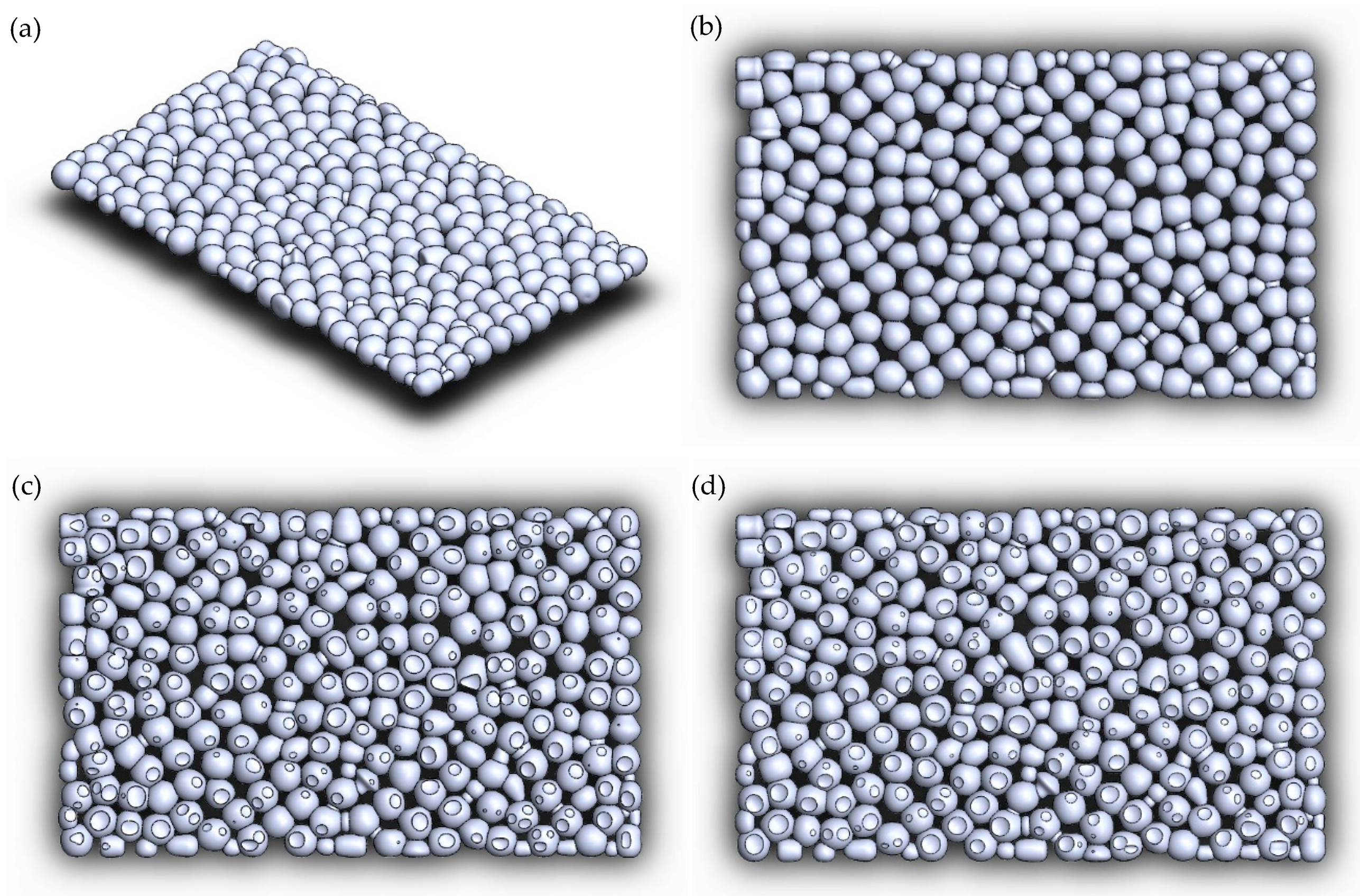
The CAD model was developed by dividing the length of the riverbed into four, 500-mm long similar elements. Thus, only one unique element, or assembly, needed to be created, with the remaining three being copies of the original. To achieve the appearance of a natural gravel riverbed, the artificial gravel particles had to be created from individual uniquely curved shapes that were devoid of any flat planes in any axis or overlap, appeared randomly positioned, and formed void spaces that varied in volume and shape. These criteria were achieved by first designing a single, 300-mm wide and 500-mm long layer of 272 uniquely shaped, nominally spherically, gravel particles with diameters between 26–30 mm, with an average diameter of 28 mm, as shown in Figure 1a,b.
Within this layer, voids between particles were formed by ensuring that individual particles overlapped by some proportion in a triangular formation, as shown by Figure 1b. This unique, original layer of artificial gravel particles was then copied four times, giving five similar layers that were then stacked at 23-mm centers and at different orientations, as detailed in Table 1(a), to form a 120-mm tall assembly. As Figure 1c,d show, the first, third, and fifth-layer geometry was taken away from the second and fourth layers, forming cavities or sockets where the geometries intersected. Thus, once machined, each layer of the riverbed would fit together with minimal interference and in the correct orientation.
At this point in the design, there were a total of 12 similar ‘whole’ geometry sheets for the first, third, and fifth layers, four similar ‘cavity’ geometry sheets for the second layer, and a further four similar ‘cavity’ geometry sheets for the fourth layer; these made up the entire artificial gravel riverbed assembly.
To realize a mating design between each assembly similar to that between the layers within those assemblies, every sheet would have to be unique. This would greatly increase the time required for setup, and the CNC cut program development by the machinist resulting in increased total manufacturing time. Therefore, without greatly increasing this time, yet preventing disjointed geometry between assemblies, three unique jointing elements were designed.
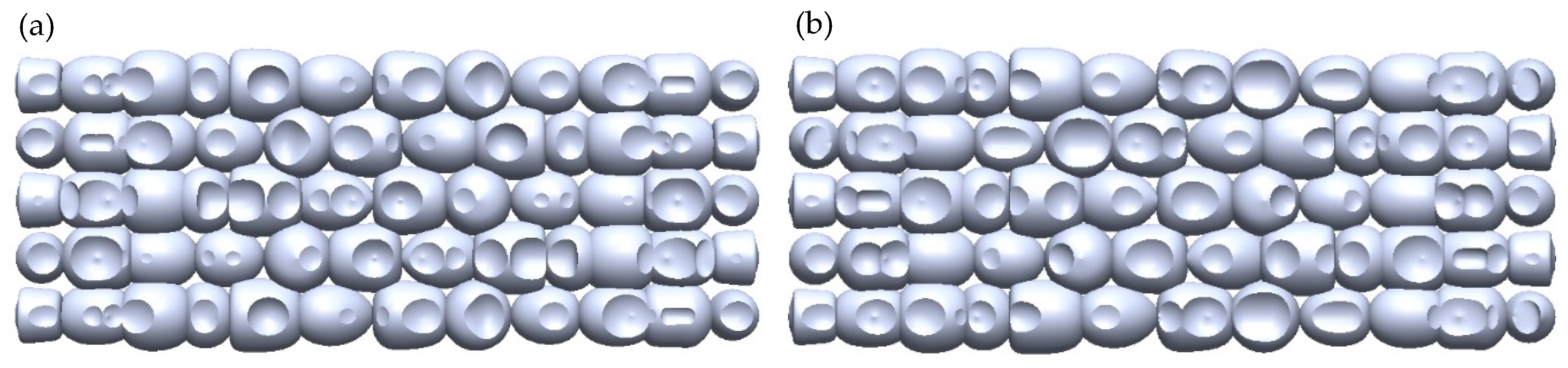
To improve the geometric variation in the streamwise direction, each assembly was orientated differently, as detailed in Table 1(b). At the joints between the assemblies three similar 120-mm tall and 300-mm wide elements, which were created in the same fashion as the layers that made up each assembly, were inserted at eight-millimeter offsets from each assembly. The solid assembly geometry was taken away from the jointing elements, forming cavities where the geometry intersects, and creating two different types of unique joint. Two of the joints are shown in Figure 2a, and one of the joints is shown in Figure 2b. Equivalent 500 mm-wide joints were also designed in a similar fashion to the 300 mm-wide joints to allow a 500 mm-wide flume to be used in later study. For the 500 mm-wide joints, each assembly was orientated in the same fashion as detailed in Table 1(b), but placed side-by-side rather than end-on-end. Finally, manufacturing and numerical simulation of the now 2.048-m long, if using 300 mm-wide joints, or 1.248-m long if using 500 mm-wide joints, artificial riverbed assembly could begin.
2.2. Physical Model Manufacturing
The CAD design outlined in Section 2.1. was used to physically manufacture an artificial gravel riverbed from a single 3.050-m long, 2.030-m wide and 30-mm thick sheet of cast acrylic. Cast acrylic was chosen for manufacturing due to it being relatively easy to machine using CNC machines; it exhibits high thermal stability, is readily available at reasonable cost, and exhibits good structural properties whilst remaining relatively lightweight and, above all else, it is transparent. Transparency was a key material requirement, as video capture inside the riverbed matrix pores is only possible with high light levels. Also, using a transparent material gives a greater possibility of viewing turbulent flow structures from outside of the flume, thus preventing any such structure from being disturbed by measurement apparatus. It should be noted that cast acrylic does discolor with time, but it can easily be rejuvenated with the application of a small amount of cutting compound. Ideally, the refractive index of the cast acrylic (1.49) would be closer to that of water at 20 °C (1.33), resulting in riverbed geometry being indistinguishable from water. Thus, similar to Dark [9], the flow across the entire width of the riverbed could be studied. However, future study using this artificial riverbed plans to only use video cameras with a focal depth of 30 mm, and so looking beyond that depth from any given camera location would not be possible, and cast acrylic could be used.
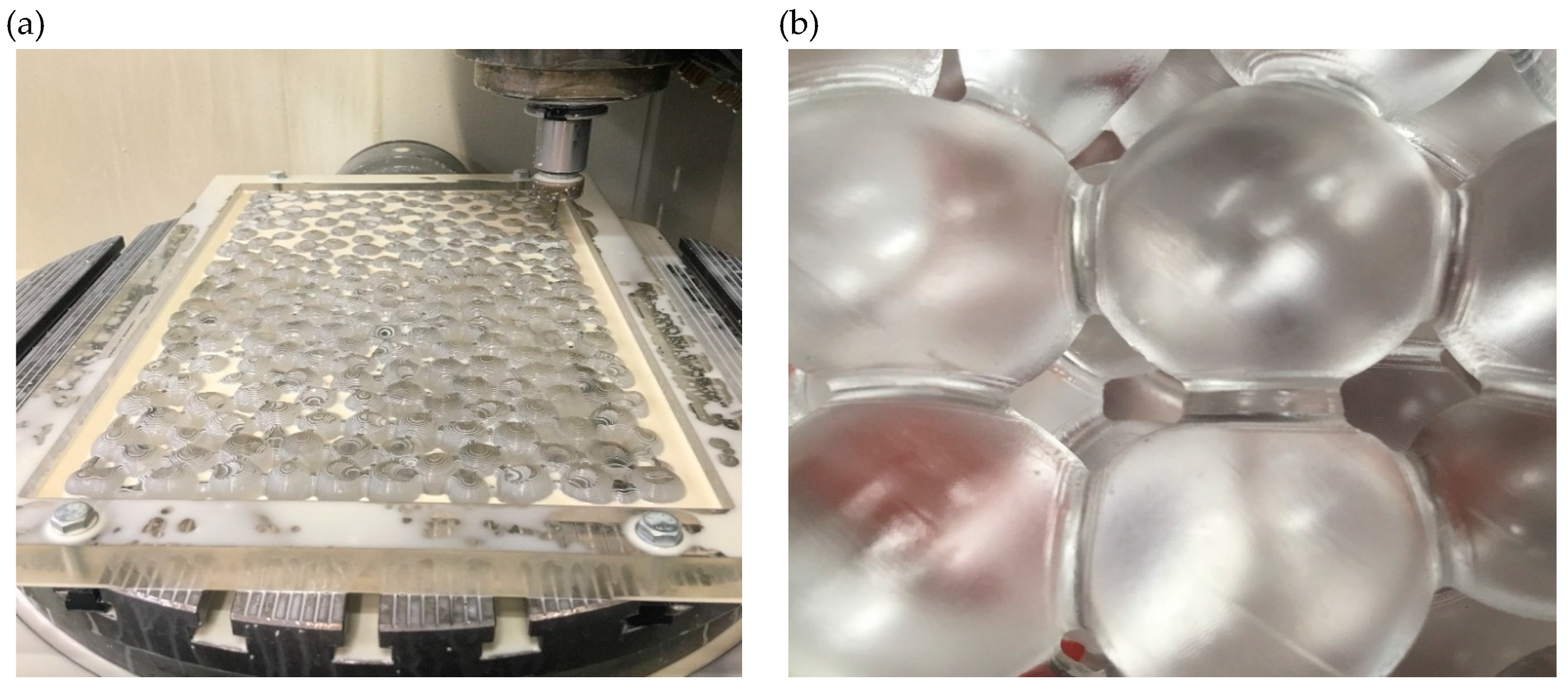
The first step in manufacturing was to cut the cast acrylic sheet into 25, 600 mm-long by 400 mm-wide plates. As explained in Section 2.1, the geometry of the artificial riverbed only required a 500 mm by 300 mm plate; however, a surrounding frame was required, as shown in Figure 3a, to allow the material to be clamped to the CNC machine bed. The riverbed geometry was connected to the frame with at least 20 evenly spaced tags, or ribs. Once clamped to either of the two five-axis CNC machines (only three-axis required) that were used, each plate was individually milled. To reduce the setup and cut programming between plates, and thus reduce the overall manufacturing time, only one side of all of the corresponding plates was milled. It was not until that side of all that layer type, as detailed in Section 2.1, were completed that the plates could be turned over, re-mounted, and the remaining sides of each plate could be milled.
The cast acrylic was machined using a 12-mm flat, long series bit for roughing out the geometry before a four-millimeter flat, long series bit was used to start forming the curvature of the geometry and pores, as shown in Figure 3a, and a three-millimeter ball end bit was used to finish the detailing. A final pass by a pencil-line program and a two-millimeter ball end bit was used to help smooth over any machining marks resulting in the completed sheet, as shown in Figure 4a. This final pencil-line program reduced the radii of the joints between any of the curved surfaces. The radii could have been further reduced with a smaller diameter bit, but at the cost of increased machining time and reduced shear strength of the plate at large, making it much more likely to fail whilst machining. The filleted material between artificial gravel particles, as shown in Figure 3b, resembles small-grained sediment particles, such as silts, that have culminated into the riverbed matrix similar to that found in nature. Thus, this specific artifact of the machining process helps to enhance the realism and representation of a natural gravel riverbed in cast acrylic. However, this is a small deviation of the physical model from the CAD model.
Upon completion of the machining, the tags between the geometry and the frame were cut, and any residual tag was filed back. It was at this point that any dimensional difference between the very small tolerance of the machining and the relatively large tolerance of the manufacture of the cast acrylic itself were dealt with. Cast acrylic is formed by pouring molten acrylic into a mold, which resulted in a relatively large degree of tolerance in material thickness over the 500-mm length of a single plate. Such dimensional variability could have been avoided by using extruded acrylic, but due to its low thermal stability resulting in poor machinability, this was not an option in this instance. With the design of the artificial riverbed consisting of nominally spherical shapes between 26–29 mm in diameter, the large tolerance in material thickness resulted in two or three small flat spots forming on each side of every plate. These were removed by sanding the affected area to a smooth convex shape. Again, this is a divergence of the physical model from that modeled using CAD. The resulting sheets could then be stacked, as described in Section 2.1, to form the four assemblies of the artificial riverbed, as shown in Figure 4b, before being placed within the flume for testing.
2.3. Numerical Model Development
The CAD model described in Section 2.1 cannot be directly imported, or simulated, into a computational flow modeling program, such as Hydro3D [20], which will be used in a later study, and instead must first undergo meshing. Meshing takes the solid surfaces described by a .STEP file exported from the CAD program and applies a series of numerical algorithms that result in the surfaces being redrawn as a series of triangular shapes with vertices that are point nodes with x, y, and z coordinates that describe a close approximation of the original CAD model surface geometry. The meshing of a single assembly of the artificial riverbed was undertaken using the meshing software Gmsh [19], with default settings in addition to using recombination for all of the triangular meshes and minimum/maximum element sizes of zero and one respectively, resulting in a mesh of 3,491,908 nodes. The output from Gmsh [19] was an unstructured mesh with large clusters of nodes around the interface between artificial gravel particles. Presently, Hydro3D’s [20] flow solver cannot compute for an unstructured geometry mesh, as more than one node could exist within the structured domain cells. Thus, the solver cannot determine which node to work with, and Hydro3D [20] terminates. Therefore, an intermediary program was required to structure the mesh output by Gmsh [19] before passing the now-structured mesh nodes to Hydro3D [20]. A Matlab script was created to undertake this secondary meshing. The Matlab script performs two distinct operations: structuring the mesh nodes and then checking the distance between all the nodes to ensure that no two nodes are closer in any axis than the cell dimensions of the fluid solver mesh that will be used in Hydro3D [20].
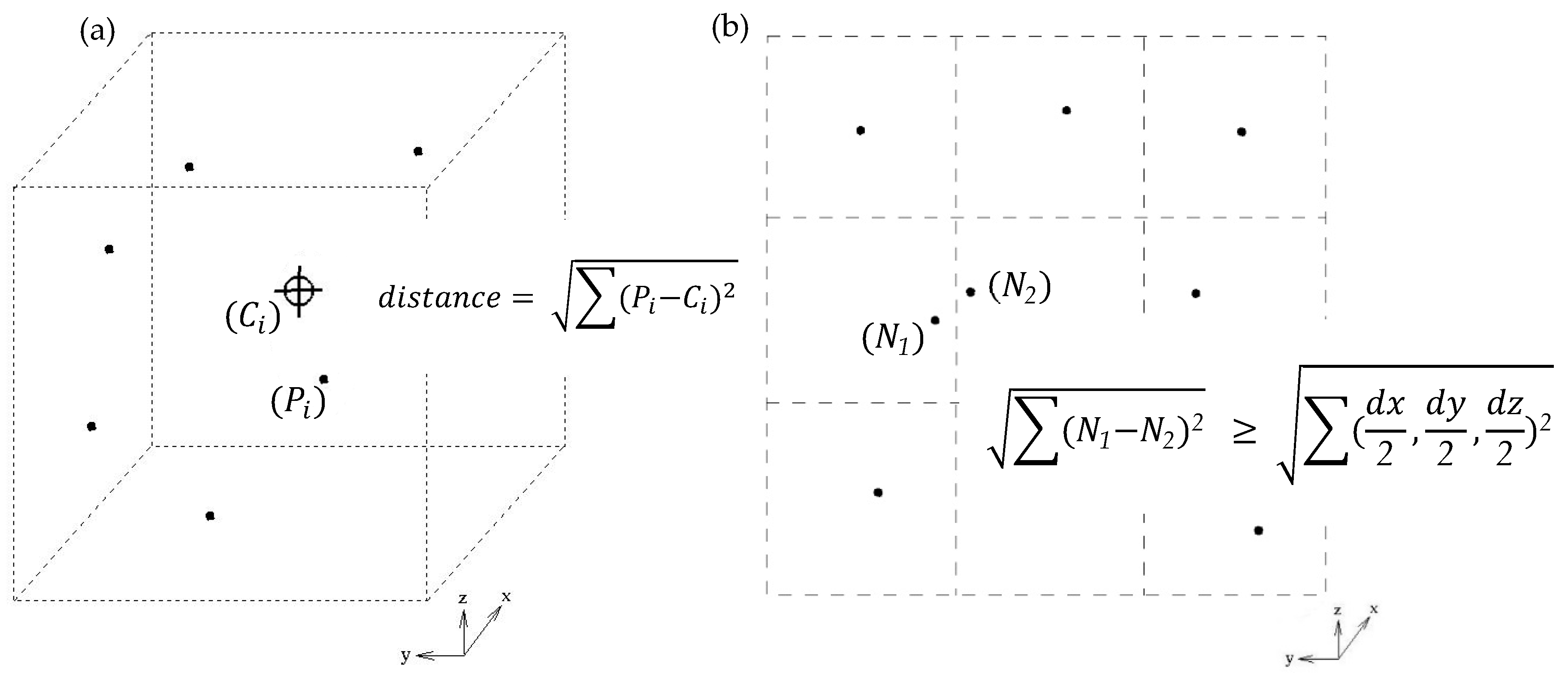
Structuring of the nodes is undertaken by searching the Gmsh [19] output and keeping only the nodes that are closest to the centers of the Hydro3D [20] fluid solver mesh cells, as shown in Figure 5a. This method retains the original node coordinates output by Gmsh [19] to achieve the best possible representation of both the CAD and physical models. Therefore, the representation is entirely determined by the degree of refinement set for the fluid solver mesh. With a desire to retain as many of the Gmsh [19] nodes as possible to better represent the geometry, a mesh refinement, or cell size, of 0.001 m in the x, y, and z axes was used. To ensure that the Gmsh [19] nodes were placed within the domain used by Hydro3D [20], origin offsets of 0.3 m in the x-direction, 0.2 m in the y-direction, and 0.05 m in the z-direction was used. The structuring of a single assembly of the artificial riverbed gave 2,188,530 nodes, which was a reduction of 37.33% compared to that output by Gmsh [19] and took approximately 39.5 h to compute using 12 cores.
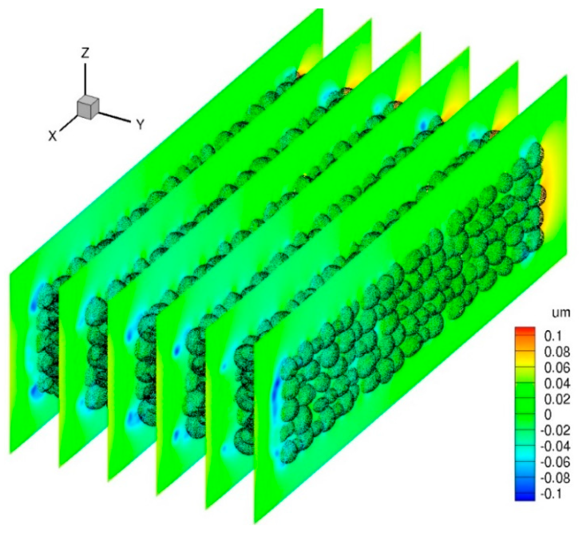
Although adjacent cells contain a single node, the distance between neighboring nodes does not necessarily conform with that required by the Hydro3D [20] fluid solver. To overcome any such issue, the distance between the nodes relative to one another was also checked. Where clusters of nodes are found using the criterion shown in Figure 5b, a new node is created, which is the centroid of that cluster. This new node, along with those already conforming, forms the list of nodes for the next iteration. Thus, the number of nodes that is retained reduces following each iteration. Iteration continues until the Euclidean distance between the node being checked and its non-conforming neighbor is within 1% of half of a cell apart, at which point they can be considered the same node. A less stringent measure of conformity might yield the same result in less time. It is only through trial and error with multiple datasets of a similar size that a more reasonable check might be found. The output from this script is a fully structured mesh that describes the artificial riverbed geometry well and complies with the requirements of Hydro3D [20], as shown by Figure 6. This mesh will allow for further computational analysis of turbulent near-bed flow along with comparison with that found experimentally using the physical model of the same artificial riverbed, as described in Section 2.2.
3. Results and Discussion
3.1. Porosity Calculation
The CAD software’s inbuilt volume calculator was used to aid the calculation of the porosity of the artificial gravel riverbed. The volume of the voids formed on the surface of the riverbed are considered by this study to be part of the channel, rather than the riverbed itself. Thus, to calculate the volume of the geometry, the surface geometry, which was determined as 0.25 d above the centerline of the uppermost layer of the artificial riverbed, was excluded, giving the volume of the geometry as 11,612.46 cm3. The total volume occupied by the geometry was calculated as 16,950 cm3, again excluding the surface geometry by using a height of 0.113 m instead of 0.12 m. Thus, the porosity of the artificial gravel riverbed was calculated using the following equation:
as 31.5%. This porosity compares well with that found by Nassrullah and Stoesser [10] for their experimentation using gravel that was on average 35 mm and 20 mm in diameter with a porosity of 31.1% and 35.8% respectively. Using the relationship:
the void ratio of the artificial riverbed was calculated as 0.46, which was at the extreme end, due to the lack of smaller particles; it was also within the maximum and minimum range for typical gravels of 0.6 to 0.3, respectively [21]. Therefore, the artificial riverbed’s pore matrix is comparable to that of a natural gravel riverbed in volume, which is a key determinant of the interstitial flowrate.
3.2. Roughness Characterization
To investigate the roughness of the artificial gravel riverbed, only the surface of the uppermost layer was used, i.e., only the surface geometry of the uppermost layer was used, which was described by nodes with a positive z-axis dimension. Using the following equations:
where:
the standard deviation in Equation (3), Fisher–Pearson coefficient of skewness in Equation (4), and excess kurtosis in Equation (5) of the artificial riverbed’s surface elevations, z(x,y), were found using an of 347,766, or the number of nodes that describe the riverbed surface geometry, as summarized in Table 2. The confidence intervals for standard deviation shown in Table 2 were calculated using the following formulae [22] (p. 245):
where:
and df is the degrees of freedom equal to N-1, and and are the chi-squared and normal distributions, respectively, for the 95% confidence level. Note that Equation (8) is only applicable if the value is greater than 30. The standard errors of skewness and kurtosis that are shown in Table 2 were calculated using the following formula:
As Table 2 shows, the variance in the size of the particles in the artificial gravel riverbed is lower than that found using natural gravel, but not as low as that used in a 2018 study [5] for their R3 roughness plate design. Given the apparent uniformity of the CAD design, as shown by Figure 1a, the standard deviation of 3.81 mm in the surface elevations is somewhat larger than expected. This is likely due to the inclusion of the much smaller than average diameter geometry that was used to improve the structural rigidity of the artificial riverbed by joining specific particles together, as shown by Figure 1b. That said, greater variance in the particle size of the artificial gravel riverbed was desirable to create a true likeness of a natural gravel riverbed. However, due to the prohibitory cost involved in obtaining thicker material, and thus more particles larger than the desired 28-mm average diameter, as well as the increased machining and setup time required, this was not possible in this study. Of course, a smaller average diameter could have been used, but at the expense of the structural rigidity of each plate, resulting in an increased risk of particle breakage whilst being machined. Thus, a reduction in the average diameter was decided against in this study.
Table 2 also shows that the skewness of the artificial gravel riverbed is close to zero, with little error due to the large population size, suggesting that the surface elevations have a normal distribution. The negative and relatively large kurtosis shown in Table 2 for the artificial gravel riverbed reflects the lack of any significant variance in the size of the gravel particles, which were particularly larger than average diameter particles, and resulting in few irregularities in the surface elevations.
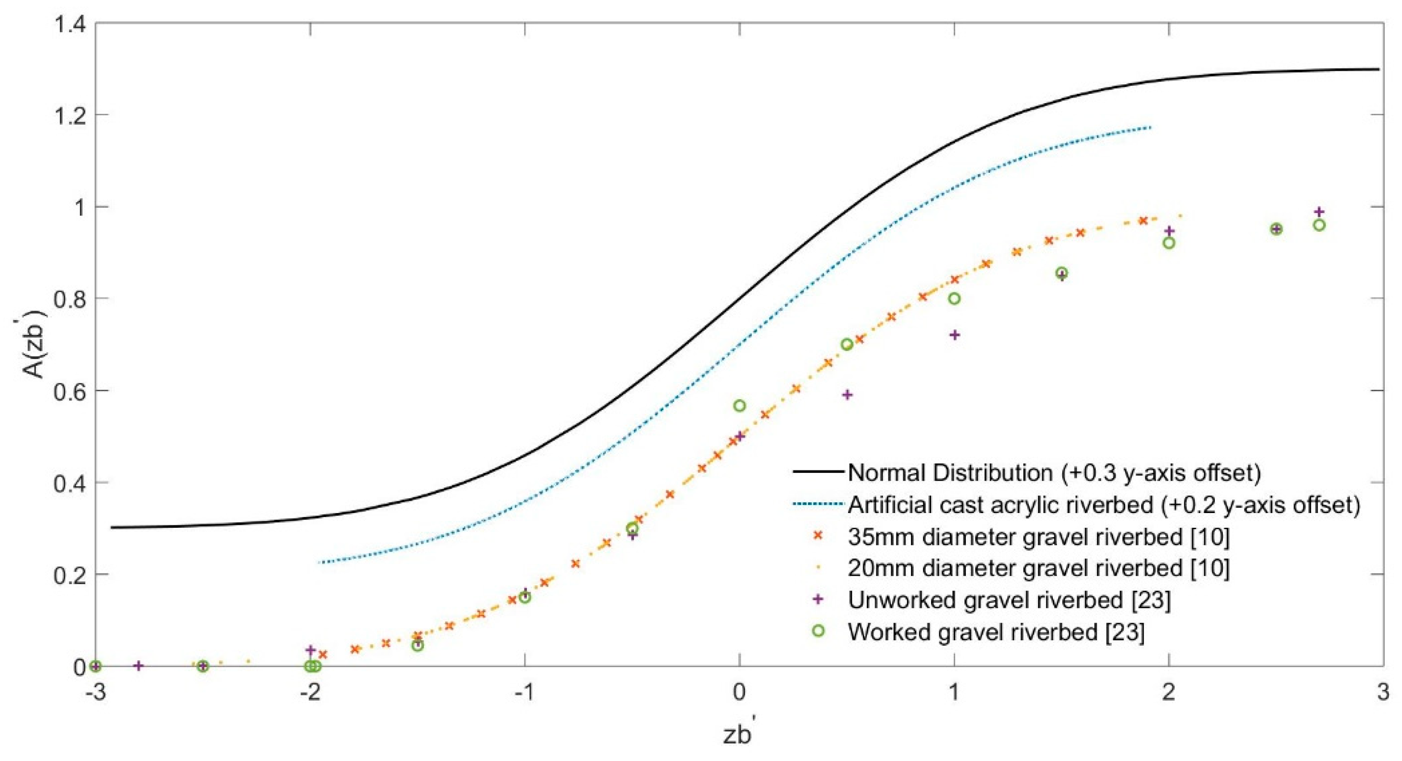
To further investigate the roughness characteristics of the artificial gravel riverbed, a roughness geometry function [3,23], which describes the cumulative probability distribution of , was utilized, and as a function of surface elevation fluctuation zb’ is plotted in Figure 7.
As Figure 7 shows, the distribution of the surface geometry elevations of the artificial gravel riverbed are near indistinguishable from those obtained by Nassrullah and Stoesser [10] for natural gravel-bed surfaces, which were either 35 mm or 20 mm in diameter, and were placed within a flume. The distribution of surface elevations found in a 2001 study [23] for both unworked gravel placed within a flume and water-worked natural riverbed gravel also correspond well to that of the artificial gravel riverbed. Equally, the distribution of surface elevations of the artificial gravel riverbed is, as expected from the result of the skewness test shown in Table 2, close to a normal distribution. The work undertaken by Aberle [1] and Aberle and Nikora [6] confirmed that the surface elevations of natural gravel riverbeds are normally distributed, thus corroborating the assertion that the artificial gravel riverbed’s surface elevation distribution is representative of that found in natural gravel riverbeds at large. Therefore, it seems reasonable to characterize the artificial riverbed as rough, with particles similarly distributed to natural gravel riverbeds. However, further analysis is required to determine how rough the artificial riverbed is in comparison to natural rivers.
The power spectral density (PSD) of a surface is often used to analyze surface roughness, as it represents the surface elevations as a function of the spatial frequency of the surface elevations where the spatial frequency, or wavevector, is the inverse of the wavelength of the surface elevations. Therefore, it provides a graphical representation of the distribution of roughness throughout a surface. Assuming that a surface is randomly rough with a Gaussian distribution, then the PSD of that surface defines its roughness characteristics [24]. If such characteristics do not vary under magnification, then the surface can be considered self-affined, and will exhibit a power-law relationship [24]:
where is the Hurst exponent related to the fractal dimension, , by . The relation expressed by Equation (11) is only true within the region:
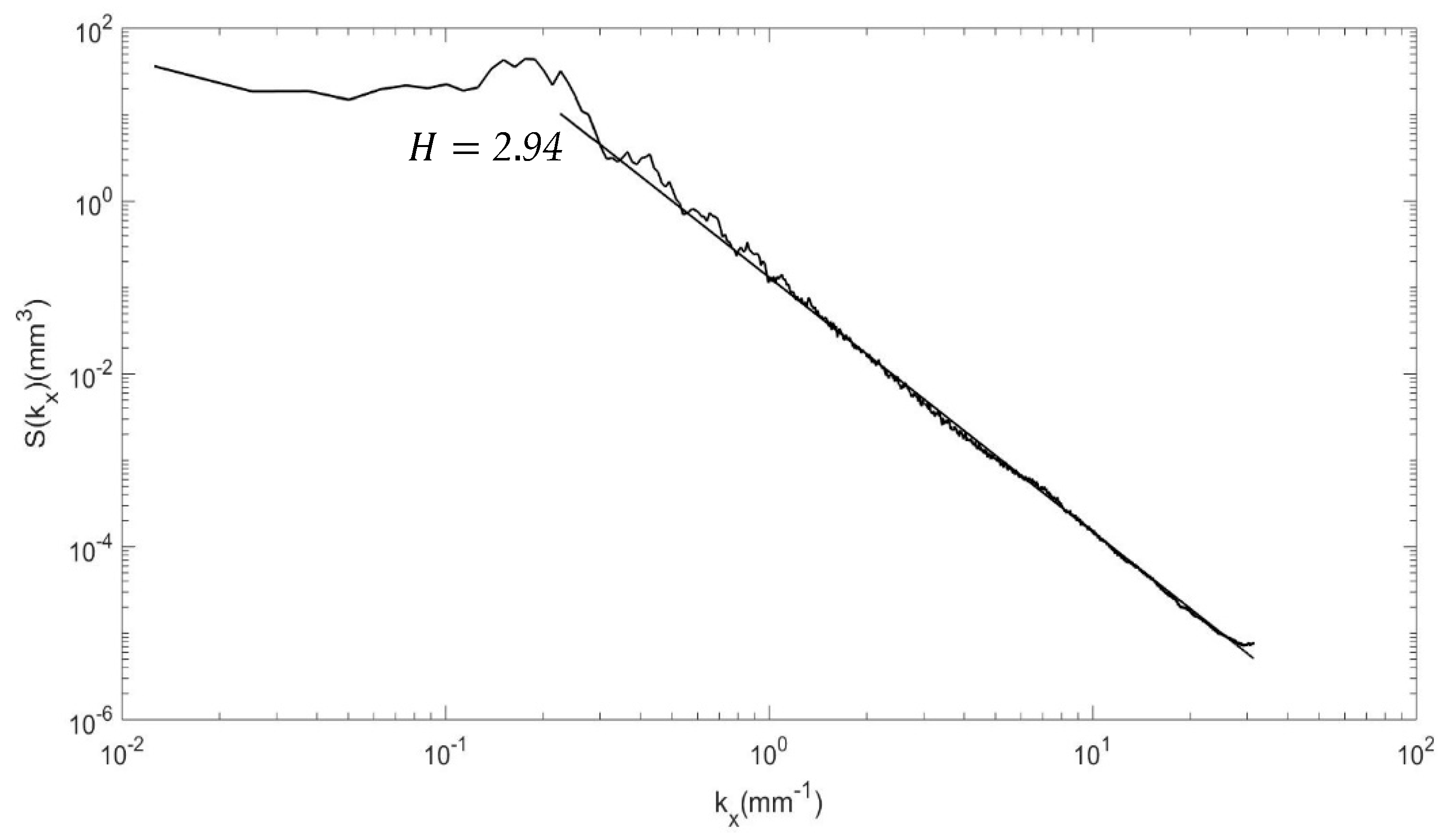
where indicates the short distance cutoff that is equal to the smallest possible wavevector corresponding to the largest particle size used, , and is the long-distance cutoff equal to the largest possible wavevector. As Persson et al. [24] suggested, for many surfaces, a value does not exist in the strict sense, as tends to a constant. Thus, can be determined from the slope of a linear regression line fitted in the region of a PSD. Using a value of 28 mm, the short distance cutoff was found to be 0.2244 for the artificial riverbed. By applying a fast Fourier transform (FFT) Matlab Function [25] to the same surface geometry used to calculate the bulk statistics of the riverbed, the PSD of the artificial riverbed was found, as shown in Figure 8.
By applying a linear regression line to the PSD in the region expressed in Equation (12), as shown in Figure 8, the Hurst exponent was found to equal 2.94. Since this value of H is greater than unity, the artificial riverbed cannot be considered a fractal at any scale [25]. Typically, H = 0.79 ± 0.04 for natural gravel-bed streams, and H = 0.50 ± 0.07 for gravel placed within a flume [26] (p. 522).
Although Figure 7 clearly shows that the distribution of roughness across the surface of the artificial gravel riverbed corresponds well with that found in nature, the Hurst exponent is much higher than that typically found in nature. As Stewart et al. [5] pointed out, the friction factor and hydraulic resistance of a riverbed decrease as the Hurst exponent increases. Thus, it can be inferred [5] that the degree of roughness of the artificial riverbed is much lower in magnitude than that found in nature. However, the value of that was found for the artificial riverbed is similar to the of 3.03 used by Stewart et al. [5] (p. 7) for their R3 roughness design.
It is clear from these results that there is some potential for enhancement of the methods developed in this study for physically and numerically approximating a natural gravel riverbed. Techniques such as photogrammetry or laser displacement scanning [5] could provide a high-resolution 3D realization of a natural water-worked gravel-bed surface. By importing the surface realization into a CAD software package, the subsurface/pore matrix of the riverbed could then be modeled, using the method described in this study, which would likely result in a very close representation of a water-worked natural gravel riverbed.
4. Conclusions
A CAD model of a gravel riverbed matrix 120 mm in depth, 300 mm wide, and 2.048 m long was created with an average particle diameter of 28 mm. Using a CNC machine, a novel physical representation of the gravel riverbed was manufactured from 25 sheets of cast acrylic. In addition, a numerical approximation of the artificial riverbed was created by applying a meshing algorithm to the CAD geometry using the open source program Gmsh [19]. The resulting mesh was then structured using a Matlab script, allowing future study of near-bed and pore-space turbulent flows using the LES code Hydro3D [20]. The artificial riverbed was then analyzed in comparison with both the natural and artificial riverbed data found in the literature. The main conclusions are:
- The porosity of the artificial riverbed was calculated as 31.5%, which compares well with the values found in the literature for natural gravel-bed surfaces. Combined with a void ratio of 0.46, which although at the extreme end due to the lack of smaller particles, is within the maximum and minimum range for typical gravels. Thus, the artificial riverbed’s pore matrix is comparable to that of a natural gravel riverbed.
- The standard deviation of the artificial riverbed’s surface elevations was found to be 3.81 mm. This suggests that the variance in particle diameter in the artificial riverbed is less than that found in natural rivers, yet larger than that used by studies found in the literature.
- The skewness and kurtosis of the artificial riverbed were calculated as –0.176 and –1.012, respectively. The skewness result suggests that the surface elevations of the artificial riverbed are normally distributed, which was confirmed by a cumulative probability distribution plot of the riverbed’s surface elevations. The negative and relatively large kurtosis relates to the lack of variance in the particle diameters used in the artificial riverbed, and thus, the lack of irregularities in the surface elevations.
- A power spectral density function was applied to the surface elevations, giving a Hurst exponent of 2.94. Thus, the artificial riverbed cannot be considered as fractal at any scale. Also, the artificial riverbed exhibits a degree of roughness that was much lower than that found in nature, meaning the hydraulic resistance and friction factor will, as a result, be lower than desired.
The results presented in this study show that the developed methods can offer both the physical and numerical approximation of a gravel bed surface comparable to a natural gravel riverbed with low surface roughness, as well as reduced particle size variance, particle distribution, and porosity within limits, but at the extreme end of the scale. These models will facilitate future experimental and computational studies of near-bed and pore-space turbulent flows.
Author Contributions
A.S. designed, developed and analysed the physical and numerical models. A.S. wrote the paper. B.B.-E. and T.S. edited the manuscript and provided scientific advice. All authors read and approved the final manuscript.
Funding
This work was supported by the Engineering and Physical Sciences Research Council in the UK via grant EP/L016214/1 awarded for the Water Informatics: Science and Engineering (WISE) Centre for Doctoral Training, which is gratefully acknowledged.
Acknowledgments
The authors wish to thank Andrew Rankmore and Cardiff University’s Mechanical Workshop for their technical support in the manufacturing of materials used in this study.
Conflicts of Interest
The authors declare no conflict of interest.
References
- Aberle, J. Measurements of armor layer roughness geometry function and porosity. Acta Geophys. 2007, 55, 23–32. [Google Scholar] [CrossRef]
- Nield, D.A.; Bejan, A. Convection in Porous Media, 5th ed.; Springer: New York, NY, USA, 2017. [Google Scholar]
- Stoesser, T. Physically Realistic Roughness Closure Scheme to Simulate Turbulent Channel Flow over Rough Beds within the Framework of LES. J. Hydraul. Eng. 2010, 136, 812–819. [Google Scholar] [CrossRef] [Green Version]
- Blois, G.; Sambrook Smith, G.H.; Best, J.L.; Hardy, R.J.; Lead, J.R. Quantifying the dynamics of flow within a permeable bed using time-resolved endoscopic particle imaging velocimetry (EPIV). Exp. Fluids 2012, 53, 51–76. [Google Scholar] [CrossRef]
- Stewart, M.T.; Cameron, S.M.; Nikora, V.I.; Zampiron, A.; Marusic, I. Hydraulic resistance in open-channel flows over self-affine rough beds. J. Hydraul. Res. 2018. [Google Scholar] [CrossRef]
- Aberle, J.; Nikora, V. Statistical properties of armored gravel bed surfaces. Water Resour. Res. 2006, 42. [Google Scholar] [CrossRef] [Green Version]
- Anderson, W.; Meneveau, C. Dynamic roughness model for large-eddy simulation of turbulent flow over multiscale, fractal-like rough surfaces. J. Fluid Mech. 2011, 679, 288–314. [Google Scholar] [CrossRef]
- Barros, J.M.; Schultz, M.P.; Flack, K.A. Measurements of skin-friction of systematically generated surface roughness. Int. J. Heat Fluid Flow 2018, 72, 1–7. [Google Scholar] [CrossRef]
- Dark, A.L. Numerical Modelling of Groundwater–Surface Water Interactions with the Double-Averaged Navier-Stokes Equations. Ph.D. Thesis, University of Canterbury, Christchurch, New Zealand, 2017. [Google Scholar]
- Nassrullah, S.; (Cardiff University, Cardiff, UK); Stoesser, T.; (University College London, London, UK). Personal communication, 2018.
- Goharzadeh, A.; Khalili, A.; Jorgensen, B.B. Transition layer thickness at a fluid-porous interface. Phys. Fluids 2005, 17. [Google Scholar] [CrossRef]
- Panah, M.; Blanchette, F. Simulating flow over and through porous media with application to erosion of particulate deposits. Comput. Fluids 2018, 166, 9–23. [Google Scholar] [CrossRef]
- Goyeau, B.; Lhuillier, D.; Gobin, D.; Velarde, M.G. Momentum transport at a fluid-porous interface. Int. J. Heat Mass Transfer 2003, 46, 4071–4081. [Google Scholar] [CrossRef]
- Khalili, A.; Basu, A.J.; Pietrzyk, U.; Raffel, M. An experimental study of recirculating flow through fluid-sediment interfaces. J. Fluid Mech. 1999, 383, 229–247. [Google Scholar] [CrossRef]
- Pokrajac, D.; Manes, C. Velocity Measurements of a Free-Surface Turbulent Flow Penetrating a Porous Medium Composed of Uniform-Size Spheres. Transp. Porous Med. 2009, 78, 367–383. [Google Scholar] [CrossRef]
- Morad, M.R.; Khalili, A. Transition layer thickness in a fluid-porous medium of multi-sized spherical beads. Exp. Fluids 2009, 46, 323–330. [Google Scholar] [CrossRef]
- Valyrakis, M.; Diplas, P.; Dancey, C.L. Entrainment of coarse particles in turbulent flows: An energy approach. J. Geophys. Res. Earth Surf. 2013, 118, 42–53. [Google Scholar] [CrossRef] [Green Version]
- Stoesser, T. Coherent flow structures: Driving Mechanism for Hyporheic Exchange over Permeable Beds? In Proceedings of the International Conference on Fluvial Hydraulics, Cesme, Turkey, 3–7 September 2008; pp. 3–5. [Google Scholar]
- Geuzaine, C.; Remacle, J.F. Gmsh: A Three-Dimensional Finite Element Mesh Generator with Built-In Pre- and Post-Processing Facilities. Int. J. Numer. Meth. Eng. 2009, 79, 1309–1331. [Google Scholar] [CrossRef]
- Ouro, P.O.; Stoesser, T. An immersed boundary-based large-eddy simulation approach to predict the performance of vertical axis tidal turbines. Comput. Fluids 2017, 152, 74–87. [Google Scholar] [CrossRef] [Green Version]
- Das, B.M. Advance Soil Mechanics, 3rd ed.; Taylor and Francis: Abingdon, UK, 2008. [Google Scholar]
- Spiegel, M.R.; Stephens, L.J. Theory and Problems of STATISTICS, 3rd ed.; McGraw-Hill: New York, NY, USA, 1999. [Google Scholar]
- Nikora, V.; Goring, D.; McEwan, I.; Griffiths, G. Spatially Averaged Open-Channel Flow Over Rough Bed. J. Hydraul. Eng. 2001, 127, 123–133. [Google Scholar] [CrossRef]
- Persson, B.N.J.; Albohr, O.; Tartaglino, U.; Volokitin, A.I.; Tosatti, E. On the nature of surface roughness with application to contact mechanics, sealing, rubber friction and adhesion. J. Phys. Condens. Matter 2005, 17, 1–62. [Google Scholar] [CrossRef] [PubMed]
- Kanafi, M.M. 1-Dimensional surface roughness power spectrum of a profile or topography. 2016. Available online: https://uk.mathworks.com/matlabcentral/fileexchange/54315-1-dimensional-surface-roughness-power-spectrum-of-a-profile-or-topography?s_tid=prof_contriblnk (accessed on 30 November 2018).
- Nikora, V.; Goring, D.G.; Biggs, B.J.F. On gravel-bed roughness characterization. Water Resour. Res. 1998, 34, 517–527. [Google Scholar] [CrossRef] [Green Version]
Figure 1.
Clockwise from top left; (a) An orthogonal view of the first layer of the artificial riverbed measuring 300 mm wide, 500 mm long, and 28 mm thick, on average; (b) The plan view of the first layer of the artificial riverbed, highlighting how particle geometry is positioned to form voids; (c) The plan view of the second layer of the artificial riverbed, highlighting the cavities left by the third layer; (d) The plan view of the fourth layer of the artificial riverbed, highlighting the cavities left by the fifth layer.

Figure 2.
(a) The side view of the jointing element between assemblies one and two, as well as assemblies three and four; (b) The side view of the jointing element between assemblies two and three.
Figure 2.
(a) The side view of the jointing element between assemblies one and two, as well as assemblies three and four; (b) The side view of the jointing element between assemblies two and three.

Figure 3.
(a) A typical plate of the artificial riverbed in the process of being machined using a 4 mm flat, long series bit including the surrounding frame required for clamping the plate to the CNC machine bed; (b) A close-up, in plan, of the artificial gravel particles highlighting the fillet detail between adjoining particles and the voids that are typically formed when the layers are stacked.

Figure 4.
(a) A typical completed sheet with the frame still attached, highlighting the optical clarity of the cast acrylic; (b) A fully stacked assembly of the artificial riverbed prior to placement within the flume, highlighting the discoloration of the cast acrylic with time.
Figure 4.
(a) A typical completed sheet with the frame still attached, highlighting the optical clarity of the cast acrylic; (b) A fully stacked assembly of the artificial riverbed prior to placement within the flume, highlighting the discoloration of the cast acrylic with time.
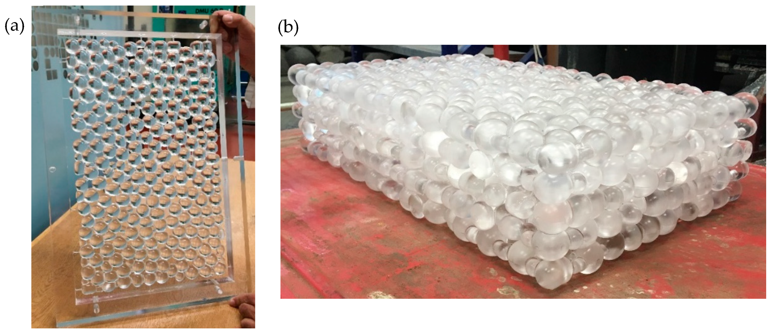
Figure 5.
(a) A diagrammatic representation of a cell and the node structuring scheme where only the node Pi(i1,j1,k1) closest to the center of the cell Ci(i2,j2,k2) is saved; (b) A diagrammatic representation of the conformity scheme for several cells, each with dimensions dx, dy and dz, where the nodes N1(i1,j1,k1) and N2(i2,j2,k2) are checked against the conformity criterion.

Figure 6.
Preliminary mean velocity results in the streamwise direction (positive x-direction) from Hydro3D [20] using the structured nodes from the Matlab script. Key Hydro3D parameters: Domain: x = 0.6 m, y = 0.4 m, z = 0.2 m; Mesh: dx, dy, dz = 0.001 m; Ubulk = 0.289 m/s; Slope = 0.001; phidepth = 0.16 m.

Figure 7.
Cumulative probability distribution of surface elevations for natural and artificial gravel riverbeds of various studies.
Figure 7.
Cumulative probability distribution of surface elevations for natural and artificial gravel riverbeds of various studies.

Figure 8.
One-dimensional surface roughness power spectral density (PSD) of the artificial gravel riverbed’s surface and a regression line between and with slope H, the Hurst exponent.
Figure 8.
One-dimensional surface roughness power spectral density (PSD) of the artificial gravel riverbed’s surface and a regression line between and with slope H, the Hurst exponent.

Table 1.
Orientation details for the layers and assemblies of the artificial riverbed.
| (a) Layer Orientation Details | (b) Assembly Orientation Details | ||
|---|---|---|---|
| Layer Number | 180° Rotation about Axis Relative to Layer 1 | Assembly Number | 180° Rotation about Axis Relative to Assembly 1 |
| 1 | None - bottom | 1 | None |
| 2 | y | 2 | y |
| 3 | z | 3 | None |
| 4 | x | 4 | y |
| 5 | None-top | ||
Table 2.
Bulk statistics of various artificial and natural gravel riverbeds, table adapted from Stewart et al. [5] (p. 7) to include multiple studies.
Table 2.
Bulk statistics of various artificial and natural gravel riverbeds, table adapted from Stewart et al. [5] (p. 7) to include multiple studies.
| Roughness Material | |||
|---|---|---|---|
| Cast acrylic artificial gravel riverbed, 28-mm diameter | 3.81 * | −0.176 (±0.004) | −1.012 (±0.008) |
| 35-mm diameter gravel [10] | 6.06 (5.50,6.77) | 0.19 (±0.18) | −0.72 (±0.37) |
| 20-mm diameter gravel [10] | 7.83 (7.28,8.48) | −0.59 (±0.13) | −0.30 (±0.27) |
| Epoxy resin artificial roughness plates, R3 design [5] | 1.58 (1.46,1.72) | −0.11 (±0.14) | 0.18 (±0.28) |
* The standard deviation for the cast acrylic artificial gravel riverbed used the entire population of nodes representing the surface geometry; thus, confidence intervals need not be calculated.
© 2018 by the authors. Licensee MDPI, Basel, Switzerland. This article is an open access article distributed under the terms and conditions of the Creative Commons Attribution (CC BY) license (http://creativecommons.org/licenses/by/4.0/).
Share and Cite
MDPI and ACS Style
Stubbs, A.; Stoesser, T.; Bockelmann-Evans, B. Developing an Approximation of a Natural, Rough Gravel Riverbed Both Physically and Numerically. Geosciences 2018, 8, 449. https://doi.org/10.3390/geosciences8120449
AMA Style
Stubbs A, Stoesser T, Bockelmann-Evans B. Developing an Approximation of a Natural, Rough Gravel Riverbed Both Physically and Numerically. Geosciences. 2018; 8(12):449. https://doi.org/10.3390/geosciences8120449
Chicago/Turabian StyleStubbs, Alex, Thorsten Stoesser, and Bettina Bockelmann-Evans. 2018. "Developing an Approximation of a Natural, Rough Gravel Riverbed Both Physically and Numerically" Geosciences 8, no. 12: 449. https://doi.org/10.3390/geosciences8120449
Note that from the first issue of 2016, this journal uses article numbers instead of page numbers. See further details here.