Detectability of Repeated Airborne Laser Scanning for Mountain Landslide Monitoring

1
Department of Earth and Atmospheric Sciences, University of Houston, Houston, TX 77204, USA
2
The Key Laboratory of Urban Security and Disaster Engineering, Beijing University of Technology, Beijing 100124, China
3
School of Civil Engineering, Tianjin Chengjian University, Tianjin 300384, China
*
Authors to whom correspondence should be addressed.
Geosciences 2018, 8(12), 469; https://doi.org/10.3390/geosciences8120469
Submission received: 17 November 2018
/
Revised: 1 December 2018
/
Accepted: 6 December 2018
/
Published: 10 December 2018
(This article belongs to the Special Issue Mountain Landslides: Monitoring, Modeling, and Mitigation)
Abstract
:Multi-temporal airborne laser scanning (ALS) surveys have become a prime consideration for detecting landslide movements and evaluating landslide risk in mountain areas. The minimum elevation change (or detectability) that can be detected by repeated ALS surveys has become a critical threshold for landslide researchers and engineers to decide if ALS is a capable tool for detecting targeted landslides and arranging the minimum time span between two scans if ALS is a choice. The National Center for Airborne Laser Mapping (NCALM) at the University of Houston conducted three repeated ALS surveys at the Slumgullion landslide site in Colorado, U.S. over one week in July of 2015. These repeated ALS surveys provide valuable datasets for evaluating the vertical detectability of multi-temporal ALS surveys in a typical mountain area. According to this study, the difference of digital elevation models (DDEM) derived from ALS has the ability of detecting a minimum elevation change of 5 cm over flatter and moderately rugged terrain areas (slope < 20 degrees) and a minimum of a 10-cm elevation change over rugged terrain areas (20 degrees < slope < 40 degrees). However, the DDEM values over highly rugged terrain areas (slope > 40 degrees), such as cliff and landslide scarps, should be interpolated with caution. Global Navigation Satellite Systems (GNSS) and Terrestrial Laser Scanning (TLS) surveys were also performed at the middle portion of the landslide area for assessing the accuracy of ALS datasets. The accuracy of ALS varies from approximately one decimeter (~10 cm) to one foot (~30 cm) depending on the roughness of terrain surface and vegetation coverage (point density). The detectability and accuracy estimates of ALS measurements obtained from the case study could be used as a reference for estimating the performance of modern ALS in mountain areas with similar topography and vegetation coverage.
1. Introduction
The use of airborne Light Detection and Ranging (LiDAR), also called airborne laser scanning (ALS), for topographic mapping, is rapidly becoming a standard practice for landslide investigations. The ability to use ALS to measure terrain surface elevations beneath a vegetated canopy has significantly advanced mountain landslide studies (e.g., [1,2,3,4,5,6]). Mountain landslides are often accompanied by significant elevation changes, which can be detected by differing repeated ALS surveys. Multi-temporal ALS surveys have become a prime consideration for detecting mass movements and monitoring land surface deformation processes (e.g., [7,8,9,10]). High-resolution bare-earth digital elevation models (DEMs) derived from ALS data often serve as the base dataset for studying terrain features. Multi-temporal DEMs can be simply subtracted by using a cell-by-cell approach to obtain elevation changes. The difference of DEMs (DDEM) has become a standard product for landslide monitoring using multi-temporal ALS and aerial photogrammetry surveys (e.g., [11,12,13]). A fundamental question about DDEM is what is the minimum elevation change (or detectability) that DDEM maps obtained from modern ALS techniques can detect? The threshold is critically important for users to decide if ALS is the right tool for detecting their targeted mass movements and for users to arrange a reasonable time span between two ALS surveys if ALS is an option. DDEM maps may not be able to detect mass movements in flatter areas and may not be able to detect slow elevation changes over a short period of time.
The precision and accuracy of ALS measurements are two fundament parameters for understanding the detectability of DDEM maps. Numerous empirical studies have been conducted to date and suggest that the elevation accuracy of ALS measurements could range from a couple of decimeters to over one meter for large-scale topographic mapping applications, depending on many issues (e.g., [14,15,16,17,18,19]). While a general understanding of the accuracy of ALS surveys is known, too few empirical studies exist for assessing the precision and accuracy of ALS point clouds in deep mountain forests.
Field measurements are always subject to certain errors or uncertainties. Precision refers to how closely repeated measurements or observations come to duplicating measured values. Therefore, precision is a measure of statistical variability or uncertainty, also called repeatability. Accuracy refers to how closely a measurement comes to matching a “true value” (trueness). Thus, accuracy is a description of observational errors. To the most stringent ALS users, field measurements need to be precise as well as accurate. In practice, it is often a challenge to precisely determine the trueness, in turn, it is difficult to assess the absolute accuracy. However, remote sensing measurements acquired by the same crew with the same equipment and processed by identical procedures may share a large portion of the uncertainty budget as common errors. Thus, DDEM maps derived from repeated ALS surveys may achieve exceptionally high accuracies in the detection of ground elevation changes.
The U.S. Geological Survey (USGS) National Geospatial Program (NGP) is responsible for updating “The National Map” of U.S. The USGS–NGP “Lidar Base Specification” (recent version 1.3, February 2018, https://pubs.usgs.gov/tm/11b4/pdf/tm11-B4.pdf) has quickly been embraced as the fundamental guidelines for Airborne LiDAR surveys of U.S. states, counties, and numerous foreign countries. The USGS LiDAR Base Specification defines four Quality Levels (QL) for ALS data. QL0 requires a vertical accuracy of 5 cm (RMSEz: vertical linear root-mean-square error in the z direction) and point density of at least 8 points/m2. QL1 and QL2 LiDAR data require a vertical accuracy of 10 cm in open terrain. QL1 requires a point density of a minimum of 8 points/m2 and QL2 requires a minimum of 2 points/m2. QL3 requires a vertical accuracy of 20 cm and a point density of 0.5 points/m2. QL2 was established as the minimum required QL for new USGS–NGP ALS data collections [20]. The USGS classification has become the national standard. Many airborne mapping companies routinely quote their survey products as QL1 LiDAR. As a consequence, non-expert LiDAR users are often educated that airborne LiDAR data would retain a 10-cm vertical accuracy. Nevertheless, experienced LiDAR users would agree that accuracy at the USGS QL1 level (~10 cm) is only achievable under the most ideal circumstances, such as low altitude flight, flat or simple terrain features, minimal or no surface vegetation or obstructions, and huge post-processing efforts. To our knowledge, the accuracy of ALS in mountain areas with complex terrain features and heavy vegetation has not been fully investigated. Most of the previous investigations focused on accuracy assessments that used ALS datasets collected in flat and open-ground surface environments.
The National Center for Airborne Laser Mapping (NCALM) at the University of Houston conducted three repeated ALS surveys over the Slumgullion landslide area in Lake City, Colorado, see Figure 1, on 3, 7, and 10 July 2015. The ALS scanned area is approximately 13 km2. These three TLS datasets were collected by the same field crew with the same equipment and were post-processed with identical procedures. They provide valuable datasets for evaluating the repeatability (precision) of model ALS surveys in a typical mountain landslide area. Static Global Navigation Satellite Systems (GNSS) surveys and Terrestrial Laser Scanning (TLS) were also performed at the middle portion of the landslide area during the ALS surveys. These ground truth measurements provide fundament datasets to assess the accuracy of the ALS datasets. The precision and accuracy of ALS surveys will help us to understand the detectability of DDEM maps.
2. ALS and TLS Data Acquisition
2.1. Study Area
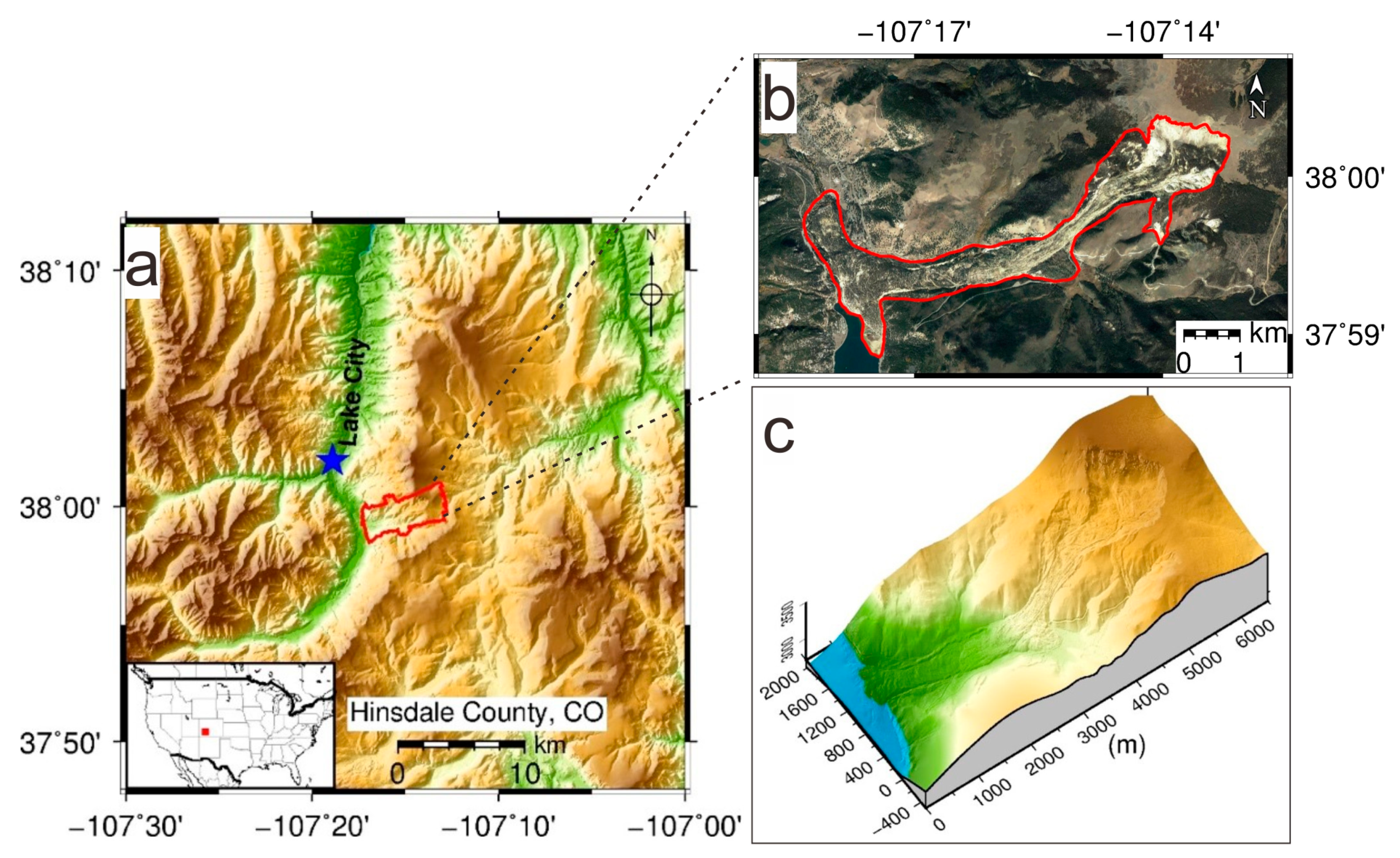
The Slumgullion landslide is located in the San Juan Mountains near Lake City, a large early-Tertiary volcanic center in Southwest Colorado, see Figure 1a. The landslide formed as a result of the collapse of hydrothermally altered volcanic materials in the rim of the Lake City Caldera. The active part of the landslide and the underlying landslide deposit are comprised of deeply weathered Tertiary basalt, rhyolite, and andesite [21]. The collapsed materials slid and flowed over 6 km downhill, thus blocked Lake Fork of the Gunnison River and created Lake San Cristobal. The Slumgullion landslide spans elevations between 2800 m and 3600 m and occupies the montane and subalpine ecological zones with sporadic coverage by Engelmann spruce and quaking aspen trees [22], see Figure 1b,c. The active part of the landslide is approximately 4-km long and 300-m wide and has an estimated volume of 2.0 × 10⁶ m3 [23]. The sliding mass has an average surface slope of 8°. The sliding speed varies in both space and time with a maximum rate of about 6–7 m/year (~1.5–2 cm/day) occurring at the narrowest part of the landslide [24]. The Slumgullion landslide has been frequently utilized as a test site for ground-based, airborne, and space-borne remote sensing studies (e.g., [25,26,27]).
2.2. ALS Data Acquisition and Processing
The ALS datasets were acquired using an Optech Gemini NIR LiDAR system installed on a Piper Chieftain PA-31 aircraft. The Optech Gemini model is capable of acquiring data at a laser pulse rate of up to 300 kHz. It records as many as four discrete returns (including the first three and last) per shot. The immediate outputs from ALS surveys are point clouds that are referenced to the kinematic positions of the onboard laser source. These “raw” point clouds are then georeferenced and processed using various algorithms. The classification of ALS point clouds is done by an automated processing algorithm using the TerraScan software package (version 16.031). The whole points are classified as ground points and non-ground points. Only the ground points, also called bare-earth points, are investigated in this study. The ALS point clouds are georeferenced to a regional East-North-Up (ENU) coordinate system. The easting (E) and northing (N) coordinates are aligned to the Universal Transverse Mercator (UTM, Zone 13N) coordinate system. The UTM coordinates in North America are referred to the geodetic reference frame North American Datum of 1983 (NAD83, epoch 2011.0) [28]. The vertical measurements (elevation) are orthometric heights calculated from the NGS GEOID12B model referred to the North American Vertical Datum of 1988 (NAVD88). The workflow for ALS data post-processing is illustrated in Figure 2. A detailed discussion regarding the NCALM field survey procedure and data quality can be referred to in a recent article published by NCALM researchers [29]. The ALS datasets from each survey were processed independently. The ALS data used for this study are archived at OpenTopography (San Diego, California, USA, http://opentopo.sdsc.edu/lidar) and are available to the public.
Figure 3 illustrates the bare-earth point clouds and a digital elevation model (DEM) derived from georeferenced ALS data acquired on 7 July 2015. The bare-earth point clouds have been down-sampled to 0.5-m by 0.5-m per point. The point with the median elevation in each grid is used to represent the location (x, y, z) of the cell if more than two points are within a grid. If only two points are within a grid, the point with the lower elevation is used to represent the location of the grid. The white grids in Figure 3a indicate the places where no ALS points exist. For convenience, the UTM coordinate system has been rotated 25° in the clockwise direction. The UTM coordinates at easting (x) 299,200 m and northing (y) 4,205,500 m were initialized to zeros in this study.
2.3. TLS Data Acquisition and Processing
TLS datasets were collected in the middle portion of the landslide area, as marked in Figure 3b. A Trimble GNSS and RIEGL VZ-2000 scanner integrated system was used for the TLS survey in the field, see Figure 4a. TLS datasets from eight scans conducted on 7 July 2015 are used for this study. Locations of these TLS scan positions are marked in Figure 5. One GNSS antenna was mounted on the top of the scanner, see Figure 4a, and another one was installed on the top of a reflector, as shown in Figure 4b. The distance between the scanner and reflector was limited to 200 m. Point clouds from each scan were registered to the ENU coordinate system using a direct georeferencing method [30]. The classification of TLS data was initially performed by a vegetation filter employed in the RiSCAN Pro. A manual process was further involved to remove certain non-ground TLS points that were not removed by the automatic filtering.
A comparison of point density (point per square meter) of bare-earth point clouds from ALS and TLS surveys (600-m by 600-m) is depicted in Figure 5a. The ALS survey yields a more uniform point distribution than the TLS survey. TLS points are mostly concentrated near the scanner positions and the point density decreases rapidly with the increase of the distance to the scanner. There are frequent and large data gaps within the TLS datasets because of the line-of-sight problem of TLS, also known as the “shadow” problem. The average point density of the bare-earth ALS points within the landslide area is about 6 to 15 points per square meter, matching the point density requirement of USGS QL1 Lidar. There are fewer ground points in areas with trees than open areas.
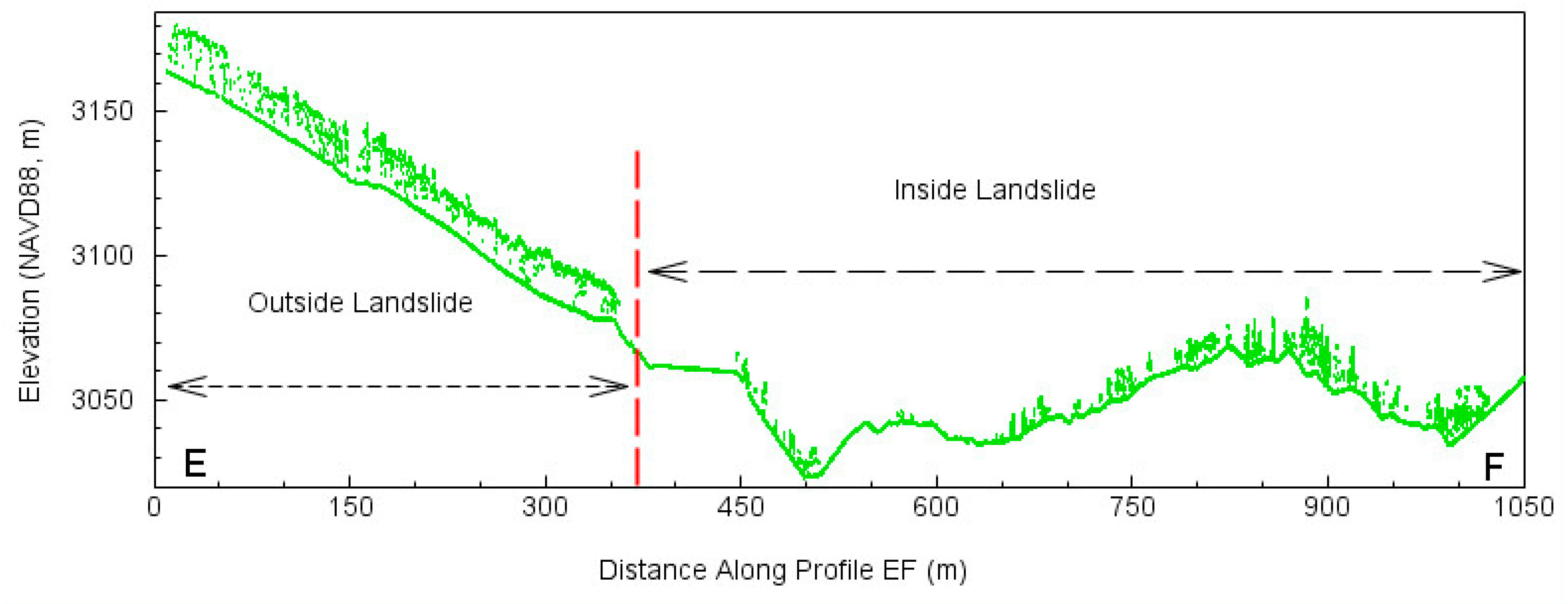
Figure 6 depicts the typical topographic features and vegetation coverage inside and outside the active portion of the landslide. The location of the profile is marked in Figure 3a. There is less vegetation inside the sliding mass but with more complex geometric terrain features compared to the areas outside the sliding mass. Landslides are known to have rougher surfaces than neighboring stable terrain due to uneven deformation of sliding mass in both the horizontal and vertical directions.
3. Difference of DEMs (DDEM)
ALS surveys provide discrete ground points that are unevenly distributed, particularly in areas with complex terrain features and vegetation coverage. For topographic surveying using ALS, the final product is often a DEM: z = f(x, y), where “z” is the ground evaluation of a point with plane coordinates x and y. DEMs are usually stored in regular grids. Certain averaging, smoothing (filtering), interpolation, and extrapolation processing are involved in generating DEMs from discrete LiDAR points. The overall accuracy of a DEM is largely a function of the field-surveying strategy, accuracy, and density of survey points, gridding resolution, method of interpolation, and the complexity (or roughness) of terrain features (e.g., [31,32,33]).
In this study, the following steps are used to generate a DEM. First, the bare-earth point clouds were blocked into small, unified grid cells with a dimension of 0.5-m by 0.5-m. The point with a median elevation is selected to represent the location of the cell. Therefore, the original coordinate (x, y, z) of this point is reserved. Second, a “surface” method in the Generic Mapping Tools (GMT) software package is employed to produce a continuous and smoothed surface [34,35]. Third, an anti-aliasing filter in a frequency domain is applied to filter the initial DEM. The low-pass cutoff wavelength of the filter is set to be four times the grid size. The details of the “surface” and anti-aliasing methods are addressed in a recent publication by Xiong et al. [36].
The grid size of 0.5-m by 0.5-m is chosen to be slightly larger than the horizontal accuracy of ALS points and have at least one measurement per grid on average. The nature of lidar data makes it difficult to assess the absolute horizontal accuracy. Conventional assessments of horizontal accuracy involve multiple flights over building corners with flat roofs and special ground targets (e.g., [37,38,39]). The horizontal errors of ALS surveys could result in considerable impacts on the observed elevations in steeper and/or complex terrain features. According to our previous investigations on NCALM’s ALS datasets [39,40], the overall horizontal accuracy of point clouds would be within 0.5 m. Thus, the grid size of 0.5-m by 0.5-m is the minimum grid size that is able to minimize the effect of the horizontal uncertainty of ALS points on DEM elevations while retaining the most detailed terrain features. According to the Nyquist–Shannon sampling theorem, a 0.5-m sampling distance will not be able to accurately model objects (terrain features) with a horizontal dimension smaller than one meter (two times the grid size or half of the sampling frequency). This study focuses on the vertical accuracy of ALS measurements.
In order to monitor movements of the sliding mass, several GNSS stations were installed on the middle portion of the landslide area during the one-week period from 3 to 10 July 2015. The observation period of GNSS data was over 6 h. Figure 7 depicts the three-component displacement time series (hourly solutions) and horizontal trajectory of a GNSS antenna (GPS1) fixed on the landslide. The relative positions are obtained by employing a double-difference carrier-phase static processing method. The locations of GPS1 and the reference GNSS station, REF0, are marked in Figure 3b. The baseline is less than 150 m. The short baseline is able to secure sub-centimeter displacement accuracy for static GNSS surveys with an occupation period of 1 h [41]. According to the GNSS measurements, the average horizontal velocity is about 1.4 cm/day towards the downhill direction during the survey period. The vertical velocity is at a level of a couple of millimeters per day. Other GNSS stations on the sliding mass also recorded similar sliding rates. The accumulated sliding displacement between two ALS surveys (7-days apart) is below one decimeter in the horizontal direction and below a couple of centimeters in the vertical direction, which is smaller than the horizontal and vertical accuracies of ALS point clouds. Accordingly, the land surface can be regarded as static during the one-week survey period.
Figure 8a depicts elevations from these three ALS surveys along profile AB shown in Figure 3a. The bare-earth point clouds have been down-sampled into unified grid cells (0.5-m by 0.5-m). A median elevation is selected to represent the elevation of the grid. The elevation varies from 2800 m to 3600 m along the 6.5-km length. Nevertheless, the differences in elevation measurements among the three surveys could not be observed from such a large-scale profile. Since the grid size is larger than the horizontal accuracy of ALS points, the elevation measurements from three surveys within the same grid (0.5-m by 0.5-m) could be regarded as the repeated measurements for the same ground point. Figure 8b illustrates the differences in the elevations between two ALS surveys on 3 July and 7 July and between two ALS surveys on 10 July and 7 July. The ALS measurements acquired on 7 July 2015 are used as references to assess the vertical precision (repeatability) of ALS surveys. Both datasets resulted in a root mean square of differences (RMSD) of approximately 9 cm, which indicates the repeatability of the vertical measurements of the ALS surveys. Figure 8c illustrates the elevation differences of two ALS-derived DEMs between 3 July and 7 July and between 10 July and 7 July 2015. The RMSD of DEMs is below 5 cm. It comes as no surprise that the overall precision of DEMs is better than the precision of discrete ALS points. The process of generating DEMs from redundant ALS points (~10 points per grid) often involves certain averaging and smoothing steps. Figure 8d illustrates the differences of elevations between the discrete ALS points (7 July 2015) and their corresponding DEM grids. Only those cells having original laser points are compared. RMSD is about 6 cm, smaller than the precision (RMSD) of the discrete ALS points, see Figure 8b.
Figure 9 depicts three DDEM maps showing an elevation difference of each of the two DEMs. The right column shows the histograms of the distribution of DDEM values. The mean of all the elevation differences across the whole scanning area is below 5 cm; the standard deviation (σ) is approximately 5 to 6 cm; the root-mean-square of the differences (RMSD) is approximately 6 to 7 cm. DDEM values over 70% of the scan area are within ±5 cm and the values over 90% of the whole scanned area are within ±10 cm. DDEM maps indicate the repeatability of ALS surveys over areas with different terrain roughnesses. Figure 10 depicts the terrain roughness of the study area. Terrain roughness is a morphometric measure expressing how heterogeneous a land surface is. The term roughness is defined and interpreted differently depending on the field of study, the scale of analysis, and the aim of application. In practice, terrain roughness can be quantified based on variations of the surface slope, the standard deviation of elevations, slope convexity, the variability of plan convexity (contour curvature), or some other measure of topographic texture. Here we define the terrain roughness as the maximum surface slope over an area of one square meter. The roughness is calculated by the GMT command “grdgradient” from the bare-earth DEM [34]. Grdgradient considers four neighbors of each DEM cell to calculate a local slope. Specifically, the points z(i − 1, j) and z(i + 1, j) are used to calculate the slope in the x-axis direction and z(i, j + 1) and z(i, j − 1) are used to calculate the slope in the y-axis direction. The final slope for each DEM cell is the square root of the sum of these two slope squares (hypotenuse). The slope represents the maximum surface slope within an area of approximately four times of the unit cell (4 × 0.25 m2). It is evident that the DDEM value is fairly consistent, except in the areas that surface roughness is significant. Sharp topographic features cannot be accurately represented by DEMs. In turn, DDEM may give false information regarding ground elevation changes in sharp topographic areas, such as cliff and landslide scarps. Large values in DDEM maps coincident with an extraordinary surface roughness (slope > 40 degrees) should be interpreted with caution.
4. Evaluating the Vertical Accuracy of ALS Data
Traditionally, georeferenced ALS datasets are evaluated against isolated ground control targets, also called checkpoints, installed at strategically important locations (e.g., [37,39]). The ground control points are surveyed by both GNSS and ALS. The contemporary method leverages a small number of isolated ground control points to quantify millions of ALS points. Statistically and practically, this method shows great weakness due to the high volume of airborne laser points being adjusted based solely on a confidence factor derived from the relationship between a segment of ALS point clouds or a portion of a DEM and several isolated ground control points. In addition to the statistical disadvantage of this method, it can be extremely difficult to identify exact ALS points that were reflected from the surface of ground control targets. Furthermore, the establishment and surveying of ground control points are often costly and time-consuming. TLS surveying has become more and more efficient and cost-effective with the development of advanced scanners, rapid field surveying and direct georeferencing methods, and automated point cloud classification (e.g., [35,42,43,44]). In general, TLS measurements can achieve a similar positional accuracy when compared to conventional ground control targets positioned by static GNSS. A single TLS scan can provide millions of credible ground references; therefore, TLS data can provide a potential alternative solution for evaluating ALS data. In this study, TLS measurements are used as references to assess the vertical accuracy of ALS measurements. According to recent experimental investigations using a similar TLS data collection and post-processing procedure, the bare-earth TLS points used for this study would be able to retain a vertical accuracy of below five centimeters and a better horizontal accuracy [30]. Well-designed TLS surveys are able to deliver sufficient accuracy for the purposes of evaluating and calibrating ALS surveys. Nevertheless, any assessment of accuracy introduces additional “apparent” error from the reference data.
Figure 11 depicts the comparisons of bare-earth elevations measured by both ALS and TLS over a portion (600-m by 600-m) of the landslide area marked in Figure 3. The point clouds have been down-sampled to 0.5-m by 0.5-m grid cells. Both ALS and TLS datasets were acquired on 7 July 2017. While the distribution of ALS points is continuous and evenly distributed in general, see Figure 11a, the TLS points are unevenly distributed with frequent large data gaps, see Figure 11b. Figure 11c,d depict the DEMs derived from the ALS and TLS points. Visually, the TLS and ALS datasets result in very similar DEMs; although, TLS has much larger data gaps than those in the ALS data. In order to precisely compare two datasets, elevations from ALS points and DEM grids along four profiles (AB, CD, EF, and GH, Figure 11b) are compared in Figure 12 and Figure 13.
The comparisons of elevation measurements from ALS and TLS points along two profiles (AB and CD) are illustrated in Figure 12. Figure 12c illustrates the differences of the point-elevations along profile AB. The differences indicate the errors of ALS points with regard to TLS measurements and only the cells that have both ALS and TLS points are compared. The mean of the errors is 4 cm with a standard deviation (σ) of 34 cm. Root mean square of errors (RMSE) retains a similar value as the standard deviation, approximately one foot (~30 cm). RMSE is computed as:
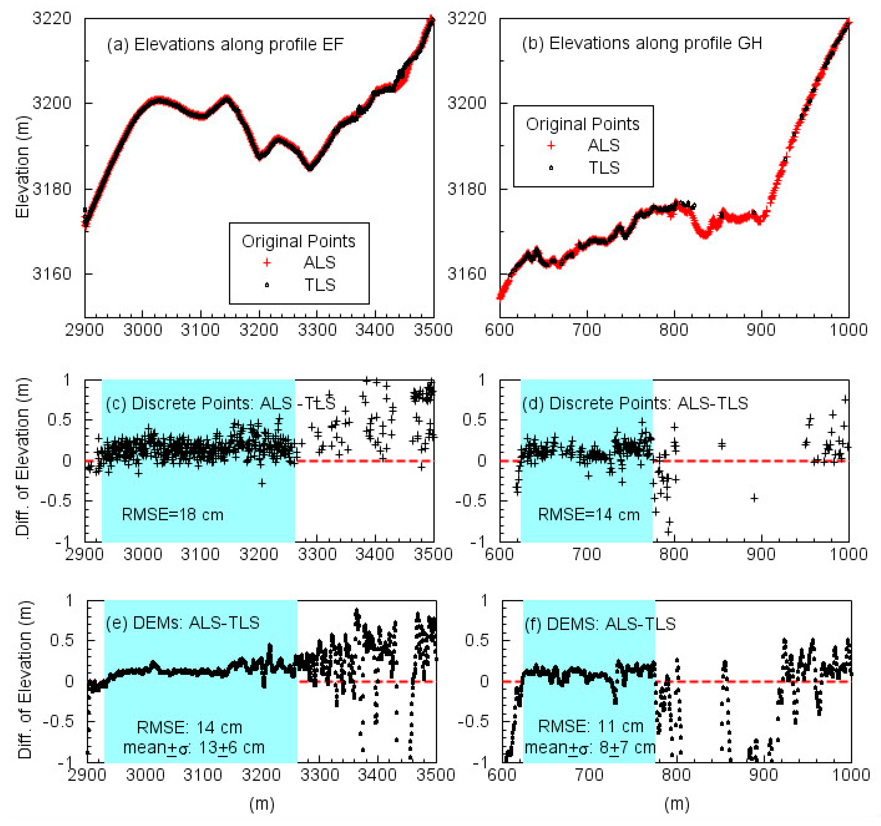
which indicates the vertical accuracy of ALS measurements. Figure 12e illustrates the differences of two DEMs along profile AB. The DEM-elevations of all cells along the profile are compared. At grid cells that have both TLS and ALS measurements, the difference between DEMs is, in general, smaller than the difference between original TLS and ALS points. However, the difference in DEMs can be considerably larger than the difference in original laser points at the places where there are no TLS measurements. This can be explained by the fact that the TLS-derived DEM can be biased by frequent data gaps in the TLS datasets. The right column of Figure 12 illustrates the same comparison for ALS and TLS datasets along profile CD.
The ground surface elevation measured by GNSS station REF1, see Figure 11b, is also marked on profile CD as a star in Figure 12b. The occupation time of REF1 was 6 h on 7 July 2015. According to the Online Positioning User Service (OPUS, https://www.ngs.noaa.gov/OPUS/) static solution, the ground elevation at REF1 is 3178.319 m with respect to NAVD88. The elevations measured by the closest (within two 0.5-m-by-0.5-m grids) TLS and ALS points are 3178.4708 m and 3178.2526 m, respectively. The elevation difference between TLS and GNSS measurements is 15 cm; the difference between ALS and GNSS measurements is 7 cm; the difference between ALS and TLS measurements is 22 cm. These three measurements agree with each other reasonably well considering the fact that the measurements were not taken at exactly the same ground point and terrain roughness can be significant at some sites, see photos in Figure 4. Figure 13 illustrates the same comparisons along another two profiles, EF and GH, see Figure 11b. There are more frequent and larger TLS data gaps along these two profiles compared to the two profiles shown in Figure 12. The comparisons along these four profiles indicate that the vertical accuracy (RMSE) of ALS points ranges from approximately 14 cm to 30 cm. The RMSE accuracy of DEMs derived from ALS points is approximately at a one-decimeter level (8 cm to 14 cm). The mean of the differences between the ALS-derived DEM and the TLS-derived DEM is approximately 10 cm, which suggests a systematic error in the ALS datasets.
5. Discussion and Conclusions
Accuracy and repeatability (precision) are two fundamental concerns for stringent ALS data users. Although ALS has been used in research and commercial mapping for almost two decades, it is still a relatively new technology since the advances in GNSS, Inertial Measurement Unit (IMU), LiDAR, software, and computing capacity have evolved continuously. ALS data processing is still an art as much as a science and it requires significant experience and manual efforts to produce highly-accurate ground surface measurements. The overall performance of ALS surveys has been continuously improving. It would be a challenge to quantify the precision and accuracy of ALS surveys, and in turn, the detectability of DDEM maps, in a simple way that keeps pace with all of these ceaseless advances.
It may not be precise to claim that the hardware (LiDAR scanner, GNSS, IMU) and methods used for this study represent the state-of-the-art of ALS technology. However, it is reasonable to say that the system (hardware + software) represents at least the average level of modern ALS technology. According to this study, modern ALS surveys could produce DDEM maps with a detectability of approximately 5-cm over flatter and moderate rugged areas (slope < 20 degrees) and a detectability of within the nearest 10-cm over rugged terrain areas (20 degrees <slope < 40 degrees). However, extraordinary elevation changes in DDEM maps coincidence with cliff and landslide scarps should be interpolated with caution. The vertical accuracy of modern ALS surveys could vary from one decimeter to one foot (~30 cm) depending on the roughness of the terrain and vegetation coverage. In general, errors are largest in areas with abrupt changes in slope. This study used three, repeated ALS datasets collected in a typical mountain landslide area by the same field crew with the same equipment and post-processed by identical procedures. Thus, the DEMs retain considerable common errors which will be canceled in DDEM. If DEMs from ALS surveys are collected by different equipment and post-processed by different methods, the detectability of DDEM maps could be worse than the result presented in this study.
The precision and accuracy results of ALS surveys from the case study could be used as a reference to evaluate ALS mapping in mountain areas with similar topography and vegetation conditions. It is critically important for non-expert LiDAR users to be aware of the complexity of ALS surveys in mountain areas and understand the spatial variation of the accuracy of ALS point clouds to avoid interpreting artifacts as true information in landslide monitoring. This is particularly important when researchers mix newly acquired ALS datasets and older datasets to produce DDEM maps. In general, old ALS datasets may retain larger errors than newly acquired datasets. We strongly suggest that users assess the accuracy of ALS datasets before using repeated ALS data to produce DDEM maps. DDEM maps are highly effective means to detect topographic changes over time only if the change calculations have accounted for measurement uncertainties.
Author Contributions
G.W., Y.B., and R.Z. designed the experiments; Y.B. managed TLS and GNSS surveys; L.X., X.Z., X.S., R.Z. performed data process and analysis; L.X. and G.W. prepared the original draft; all authors reviewed and edited the manuscript.
Funding
This research was funded by National Science Foundation of U.S., grant numbers EAR-1043051, DUE-1243582 and OISE-1460034, and National Science Foundation of China, grant number 51829801.
Acknowledgments
The authors acknowledge the work of NCALM engineers Juan Carlos Fernandez Diaz, Michael Sartori, Abhinav Singhania and Darren Hauser for collecting, processing and delivering ALS data to the public through Open Topography (http://www.opentopography.org). Hongki Lee and graduate students (Ning Cao, Timothy J. Kearns, Hanlin Liu, Xinxiang Zhu, Modurodoluwa Okeowo, Andrew Lyda, and Veronica Guzman) at the University of Houston assisted in the field surveys. UNAVCO provided GNSS equipment through its equipment loan program (EAR-0350028, EAR-0732947EAR-1042906/9).
Conflicts of Interest
The authors declare no conflict of interest.
References
- Glennie, C.L.; Carter, W.E.; Shrestha, R.L.; Dietrich, W.E. Geodetic imaging with airborne LiDAR: The Earth’s surface revealed. Rep. Prog. Phys. 2013, 76, 086801. [Google Scholar] [CrossRef]
- Glenn, N.F.; Streutker, D.R.; Chadwick, D.J.; Thackray, G.D.; Dorsch, S.J. Analysis of LiDAR derived topographic information characterizing and differentiating landslide morphology and activity. Geomorphology 2005, 73, 131–148. [Google Scholar] [CrossRef]
- Wooten, R.M.; Latham, R.S.; Witt, A.C.; Douglas, T.J.; Gillon, K.A.; Fuemmeler, S.J.; Bauer, J.B.; Nickerson, J.G.; Reid, J.C. Landslide hazard mapping in North Carolina—Geology in the interest of public safety and informed decision making. Geol. Soc. Am. Abst. Programs 2007, 39, 76. [Google Scholar]
- Eeckhaut, M.; Poesen, J.; Verstraeten, G.; Vanacker, V.; Nyssen, J.; Moeyersons, J.; Van Beek, L.P.H.; Vandekerckhove, L. Use of LIDAR-derived images for mapping old landslides under forest. Earth Surf. Proc. Land. 2007, 32, 754–769. [Google Scholar] [CrossRef]
- Razak, K.A.; Straatsma, M.W.; Van Westen, C.J.; Malet, J.P.; De Jong, S.M. Airborne laser scanning of forested landslides characterization: Terrain model quality and visualization. Geomorphology 2011, 126, 186–200. [Google Scholar] [CrossRef]
- Wang, G. Millimeter-accuracy GPS landslide monitoring using precise point positioning with single receiver phase ambiguity resolution: A case study in Puerto Rico. J. Géod. Sci. 2013, 3, 22–31. [Google Scholar] [CrossRef]
- DeLong, S.B.; Prentice, C.S.; Hilley, G.E.; Ebert, Y. Multitemporal ALSM change detection, sediment delivery, and process mapping at an active earthflow. Earth Surf. Process. Landf. 2012, 37, 262–272. [Google Scholar] [CrossRef]
- Toth, C.K.; Mora, O.E.; Lenzano, M.G.; Grejner-Brzezinska, D.A.; Beach, K. Landslide hazard detection from LiDAR data. In Proceedings of the ASPRS 2013 Annual Conference, Baltimore, MD, USA, 24–28 March 2013. [Google Scholar]
- Mora, O.E.; Liu, J.K.; Gabriela Lenzano, M.; Toth, C.K.; Grejner-Brzezinska, D.A. Small landslide susceptibility and hazard assessment based on Airborne LiDAR data. Photogramm. Eng. Remote Sens. 2015, 81, 239–247. [Google Scholar] [CrossRef]
- Mora, O.E.; Lenzano, M.G.; Toth, C.K.; Grejner-Brzezinska, D.A.; Fayne, J.V. Landslide change detection based on multi-temporal Airborne LiDAR-derived DEMs. Geosciences 2018, 8, 23. [Google Scholar] [CrossRef]
- Tseng, C.; Lin, C.; Stark, C.P.; Liu, J.; Fei, L.; Hsieh, Y. Application of a multi-temporal, LiDAR-derived, digital terrain model in a landslide-volume estimation. Earth Surf. Process. Land. 2013, 38, 1587–1601. [Google Scholar] [CrossRef]
- Müller, J.; Gärtner-Roer, I.; Thee, P.; Ginzler, C. Accuracy assessment of airborne photogrammetrically derived high-resolution digital elevation models in a high mountain environment. ISPRS J. Photogramm. Remote Sens. 2014, 98, 58–69. [Google Scholar] [CrossRef]
- Hsieh, Y.; Chan, Y.; Hu, J. Digital elevation model differencing and error estimation from multiple sources: A case study from the Meiyuan Shan landslide in Taiwan. Remote Sens. 2016, 8, 199. [Google Scholar] [CrossRef]
- Shrestha, R.L.; Carter, W.E.; Lee, M.; Finer, P.; Sartori, M. Airborne laser swath mapping: Accuracy assessment for surveying and mapping applications. J. Am. Congr. Surv. Mapp. 1999, 59, 83–94. [Google Scholar]
- Slatton, K.C.; Carter, W.E.; Shrestha, R.L.; Dietrich, W. Airborne laser swath mapping: Achieving the resolution and accuracy required for geosurficial research. Geophys. Res. Lett. 2007, 34, L23S10. [Google Scholar] [CrossRef]
- Adams, J.; Chandler, J. Evaluation of LiDAR and medium scale photogrammetry for detecting soft-cliff coastal change. Photogramm. Rec. 2002, 17, 405–418. [Google Scholar] [CrossRef]
- Bowen, Z.H.; Waltermire, R.G. Evaluation of light detection and ranging (LiDAR) for measuring river corridor topography. J. Am. Water Resour. Assoc. 2002, 38, 33–41. [Google Scholar] [CrossRef]
- Hodgson, M.E.; Jensen, J.R.; Schmidt, L.; Schill, S.; Davis, B. An evaluation of LiDAR- and IFSAR-derived digital elevation models in leaf-on conditions with USGS Level 1 and Level 2 DEMs. Remote Sens. Environ. 2003, 84, 295–308. [Google Scholar] [CrossRef]
- Montealegre, A.; Lamelas, M.; Riva, J. Interpolation routines assessment in ALS-derived digital elevation models for forestry applications. Remote Sens. 2015, 7, 8631–8654. [Google Scholar] [CrossRef]
- Heidemann, K.H. Lidar Base Specification (Ver. 1.3, February 2018): US Geological Survey Techniques and Methods; US Geological Survey: Sioux Falls, SD, USA, 2018; Book 11, Chapter B4.
- Lipman, P.W. Geologic Map of the Lake City Caldera area, Western San Juan Mountains, Southwestern Colorado; Miscellaneous Investigations Series Map I-962, Scale 1:48,000; U.S. Geological Survey: Reston, VA, USA, 1976.
- Löve, D. Subarctic and subalpine: Where and what? Arct. Alp. Res. 1970, 2, 63–73. [Google Scholar] [CrossRef]
- Parise, M.; Guzzi, R. Volume and Shape of the Active and Inactive Parts of the Slumgullion Landslide, Hinsdale County, Colorado; U.S. Geological Survey Open-File Report; U.S. Geological Survey: Reston, VA, USA, 1992; 29p.
- Baum, R.L.; Fleming, R.W. Kinematic studies of the Slumgullion landslide, Hinsdale County, Colorado. In The Slumgullion Earth Flow: A Large Scale Natural Laboratory, 1st ed.; U.S. Geological Survey Bulletin 2130; Varnes, D.J., Savage, W.Z., Eds.; United States Government Printing Office: Washington, DC, USA, 1996; pp. 9–12. [Google Scholar]
- Delbridge, B.G.; Burgmann, R.; Fielding, E.J.; Hensley, S.; Schulz, W.H. Three-dimensional surface deformation derived from airborne interferometric UAVSAR: Application to the Slumgullion landslide. J. Geophys. Res. Solid Earth 2016, 121, 3951–3977. [Google Scholar] [CrossRef]
- Schulz, W.H.; Coe, J.A.; Ricci, P.P.; Smoczyk, G.M.; Shurtleff, B.L.; Panosky, J. Landslide kinematics and their potential controls from hourly to decadal timescales: Insights from integrating ground-based InSAR measurements with structural maps and long-term monitoring data. Geomorphology 2017, 285, 121–136. [Google Scholar] [CrossRef]
- Cao, N.; Lee, H.; Zaugg, E.; Shrestha, R.; Carter, W.; Glennie, C.; Wang, G.; Lu, Z.; Fernandez-Diaz, F.C. Airborne DInSAR results using time-domain Backprojection algorithm: A case study over the Slumgullion Landslide in Colorado with validation using Spaceborne SAR, Airborne LiDAR, and ground-based observations. IEEE J. Sel. Topics Appl. Earth Observ. Remote Sens. 2017, 10, 4987–5000. [Google Scholar] [CrossRef]
- Wang, G.; Soler, T. Measuring land subsidence using GPS: Ellipsoid height vs. orthometric height. J. Surv. Eng. 2014, 141, 05014004. [Google Scholar] [CrossRef]
- Fernandez-Diaz, J.; Carter, W.; Shrestha, R.; Glennie, C. Now you see it… Now you don’t: Understanding airborne mapping LiDAR collection and data product generation for archaeological research in Mesoamerica. Remote Sens. 2014, 6, 9951–10001. [Google Scholar] [CrossRef]
- Xiong, L.; Bao, L.; Wang, G.; Zhou, X.; Sun, X.; Zhao, R. Evaluation of a rapid TLS surveying method for coastal erosion monitoring: A case study at Freeport, Texas. J. Surv. Eng. 2018. submitted. [Google Scholar]
- Anderson, E.S.; Thompson, J.A.; Austin, R.E. LIDAR density and linear interpolator effects on elevation estimates. Int. J. Remote Sens. 2005, 26, 3889–3900. [Google Scholar] [CrossRef]
- Guo, Q.; Li, W.; Yu, H.; Alvarez, O. Effects of topographic variability and Lidar sampling density on several DEM interpolation methods. Photogramm. Eng. Remote Sens. 2010, 76, 701–712. [Google Scholar] [CrossRef]
- Spaete, L.P.; Glenn, N.F.; Derryberry, D.R.; Sankey, T.T.; Mitchell, J.J.; Hardegree, S.P. Vegetation and slope effects on accuracy of a LiDAR-derived DEM in the sagebrush steppe. Remote Sens. Lett. 2011, 2, 317–326. [Google Scholar] [CrossRef]
- Wessel, P.; Smith, W.H.F. The Generic Mapping Tools Technical Reference and Cookbook. Version 4.5.16. Available online: https://www.soest.hawaii.edu/gmt/gmt/pdf/GMT_Docs.pdf (accessed on 12 November 2018).
- Zhou, X.; Wang, G.; Bao, Y.; Xiong, L.; Guzman, V.; Kearns, T.J. Delineating beach and dune morphology from massive terrestrial laser scanning data using the Generic Mapping Tools. J. Surv. Eng. 2017, 143, 04017008. [Google Scholar] [CrossRef]
- Xiong, L.; Wang, G.; Wessel, P. Anti-aliasing filtering for deriving high-accuracy DEMs from TLS data: A case study from Freeport, Texas. Comput. Geosci. 2017, 100, 125–134. [Google Scholar] [CrossRef]
- Csanyi, N.; Toth, C.K. Improvement of lidar data accuracy using Lidar-specific ground targets. Photogramm. Eng. Remote Sens. 2007, 73, 385–396. [Google Scholar] [CrossRef]
- Cheng, L.; Tong, L.; Li, M.; Liu, Y. Semi-automatic registration of airborne and terrestrial laser scanning data using building corner matching with boundaries as reliability check. Remote Sens. 2013, 5, 6260–6283. [Google Scholar] [CrossRef]
- Wang, G.; Joyce, J.; Phillips, D.; Shrestha, R.; Carter, W. Delineating and defining the boundaries of an active landslide in the rainforest of Puerto Rico using a combination of airborne and terrestrial LIDAR data. Landslides 2013, 10, 503–513. [Google Scholar] [CrossRef]
- Fernandez-Diaz, J.C.; Carter, W.; Shrestha, R.; Glennie, C. Lidar remote sensing. In Handbook of Satellite Applications; Pelton, J.N., Madry, S., Camacho-Lara, S., Eds.; Springer: Berlin, Germany, 2013; Volume 2, pp. 757–808. ISBN 978-1-4419-7670-3. [Google Scholar]
- Wang, G. Kinematics of the Cerca del Cielo, Puerto Rico landslide derived from GPS observations. Landslides 2012, 9, 117–130. [Google Scholar] [CrossRef]
- Wang, G.; Philips, D.; Joyce, J.; Rivera, F.O. The integration of TLS and continuous GPS to study landslide deformation: A case study in Puerto Rico. J. Geod. Sci. 2011, 1, 25–34. [Google Scholar] [CrossRef]
- Gallay, M.; Lloyd, C.D.; McKinley, J.; Barry, L. Assessing modern ground survey methods and airborne laser scanning for digital terrain modelling: A case study from the Lake District, England. Comput. Geosci. 2013, 51, 216–227. [Google Scholar] [CrossRef] [Green Version]
- Baltensweiler, A.; Walthert, L.; Ginzler, C.; Sutter, F.; Purves, T.S.; Hanewinkel, M. Terrestrial laser scanning improves digital elevation models and topsoil pH modelling in regions with complex topography and dense vegetation. Environ. Model. Softw. 2017, 95, 13–21. [Google Scholar] [CrossRef]
Figure 1.
(a) A topographic map showing the location of the Slumgullion landslide located in the San Juan Mountains within Hinsdale County, Southwestern Colorado. The red box indicates the area covered by three ALS scans on 3, 7, and 10 July 2015. The elevation data (1/3 arc-second digital elevation model (DEM)) is from U.S. Geological Survey (https://viewer.nationalmap.gov). (b) A Google Earth image showing the vegetation coverage in the landslide area. (c) A 3D digital elevation model (DEM) showing the extension of the Slumgullion landslide in space. The DEM is derived from the bare-earth ALS data collected on 7 July 2015. The unit of the three axes is in meters.

Figure 2.
The workflow for airborne laser scanning (ALS) data post-processing.

Figure 3.
(a) A topographic map depicting bare-earth ALS point clouds collected on 7 July 2015. The ALS points have been down-sampled to 0.5-m by 0.5-m grids. Stars indicate Global Navigation Satellite Systems (GNSS) stations that were installed for georeferencing Terrestrial Laser Scanning (TLS) points. (b) A shaded relief map from a bare-earth DEM derived from the ALS points shown in (a). The red square shows the area that was also scanned by TLS on 7 July 2015.

Figure 4.
Photos showing GNSS and TLS equipment used for the TLS survey. (a) A Trimble R10 GNSS unit and a RIEGL VZ-2000 laser scanner that were mounted on a 4-m-high elevating tripod; (b) A cylinder laser reflector (20-cm in diameter, 25-cm in height) and a Trimble Zephyr 2 Geodetic GNSS antenna (paired with a Trimble NetR9 receiver).
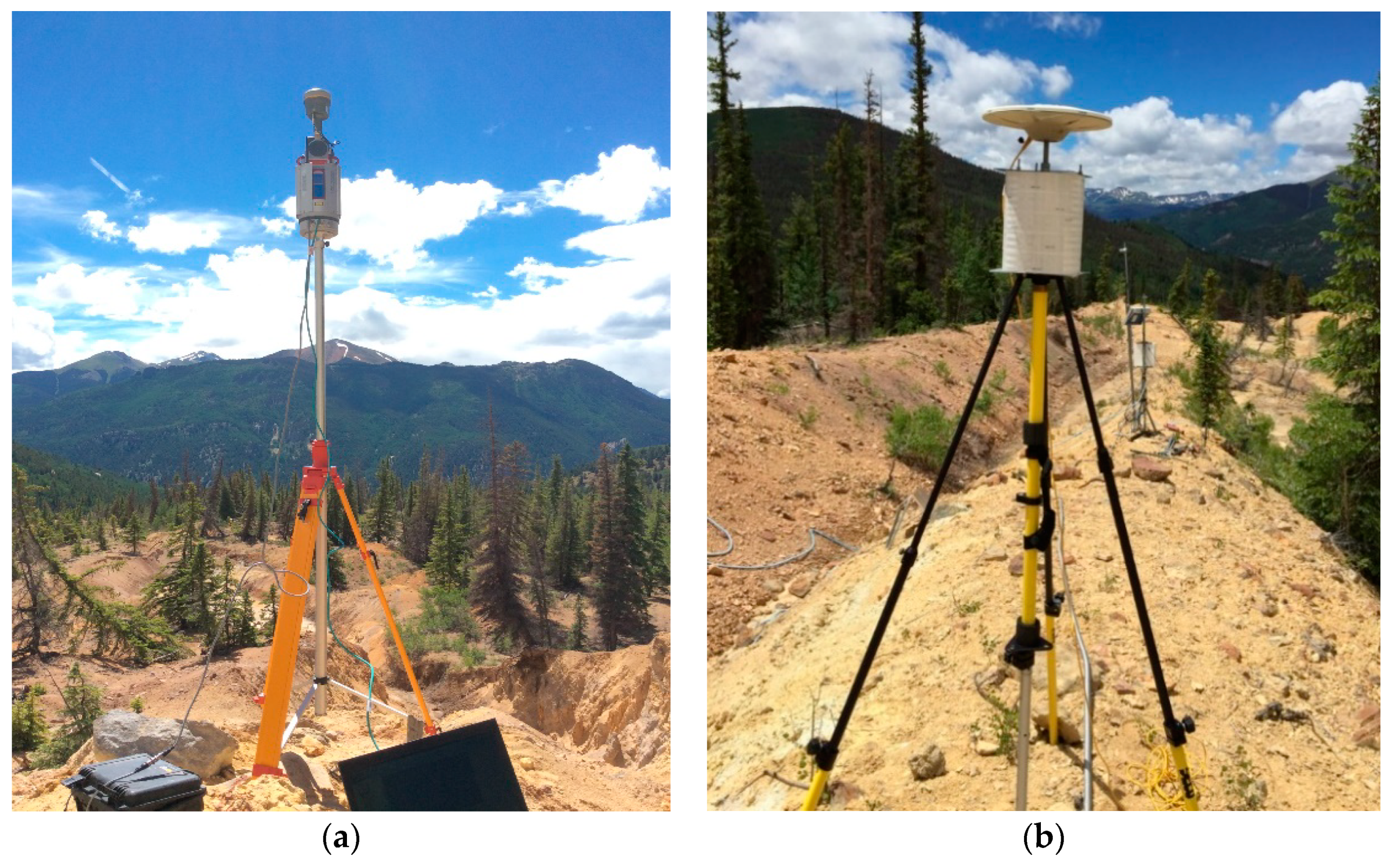
Figure 5.
A comparison of the point density of bare-earth point clouds obtained from ALS and TLS surveys on 7 July 2015. The location of the area is marked in Figure 3. The filled dark circles in (b) indicate TLS scan positions.
Figure 5.
A comparison of the point density of bare-earth point clouds obtained from ALS and TLS surveys on 7 July 2015. The location of the area is marked in Figure 3. The filled dark circles in (b) indicate TLS scan positions.

Figure 6.
Typical terrain features and vegetation coverage inside and outside the sliding mass illustrated by ALS point clouds. The location of the profile EF is marked on Figure 3a.
Figure 6.
Typical terrain features and vegetation coverage inside and outside the sliding mass illustrated by ALS point clouds. The location of the profile EF is marked on Figure 3a.

Figure 7.
(a) Three-component (NS: north to south, EW: east to west; Vertical) displacement time series of the GNSS antenna (GPS1) during the period from 3 to 10 July 2015. The displacements are referred to a GNSS station (REF0) located outside of the sliding mass. (b) The horizontal trajectory of the GNSS antenna (GPS1) during the same period as (a). Locations of GPS1 and REF0 are marked in Figure 3b.

Figure 8.
Plots illustrating the vertical precision of bare-earth ALS points. The point clouds have been down-sampled into unified grid cells (0.5-m by 0.5-m). (a) Elevation measurements from three ALS surveys along profile AB (Figure 3a). (b) Elevation differences of discrete points between two ALS surveys on 3 July and 7 July, and 10 July and 7 July 2015. (c) Elevation differences of two DEMs (DDEM) along with profile AB. (d) Elevation differences between ALS points and gridded DEM points.
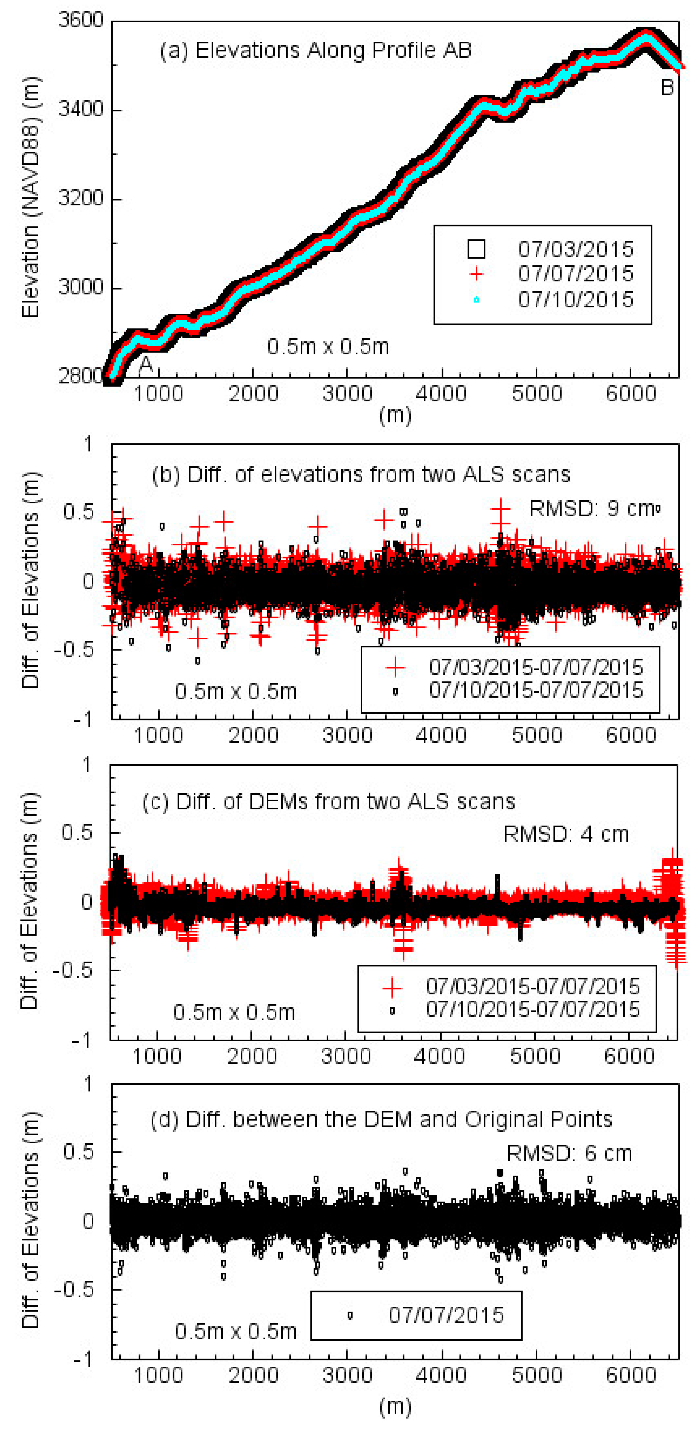
Figure 9.
The elevation difference of two DEMs (DDEM, 0.5-m by 0.5-m) derived from bare-earth ALS datasets. (a) DDEM derived from ALS surveys on 10 July and 3 July; (b) DDEM derived from ALS surveys on 10 July and 7 July; (c) DDEM derived from ALS surveys on 3 July and 7 July. The black dotted line depicts the boundary of the landslide. The unit of the difference of elevations is a centimeter. The histogram illustrates the distribution of the values of the corresponding DDEM.
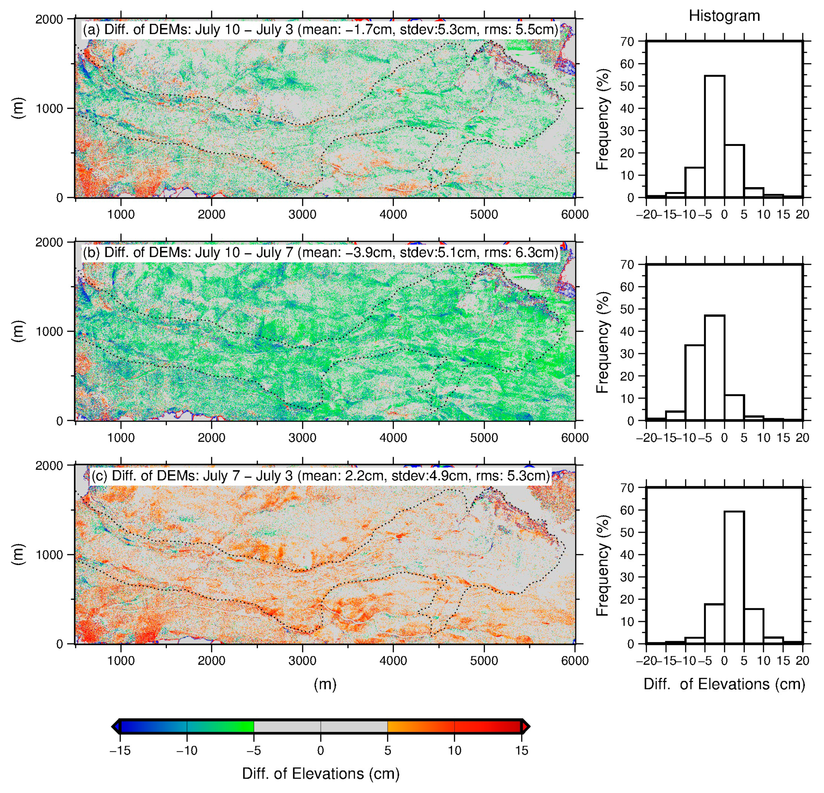
Figure 10.
Map showing the elevation contours (in meters) and the terrain roughness (in degrees) derived from the DEM on 7 July 2015. The roughness is defined as the maximum surface slope over one square meter. The blue dashed line depicts the boundary of the landslide.
Figure 10.
Map showing the elevation contours (in meters) and the terrain roughness (in degrees) derived from the DEM on 7 July 2015. The roughness is defined as the maximum surface slope over one square meter. The blue dashed line depicts the boundary of the landslide.
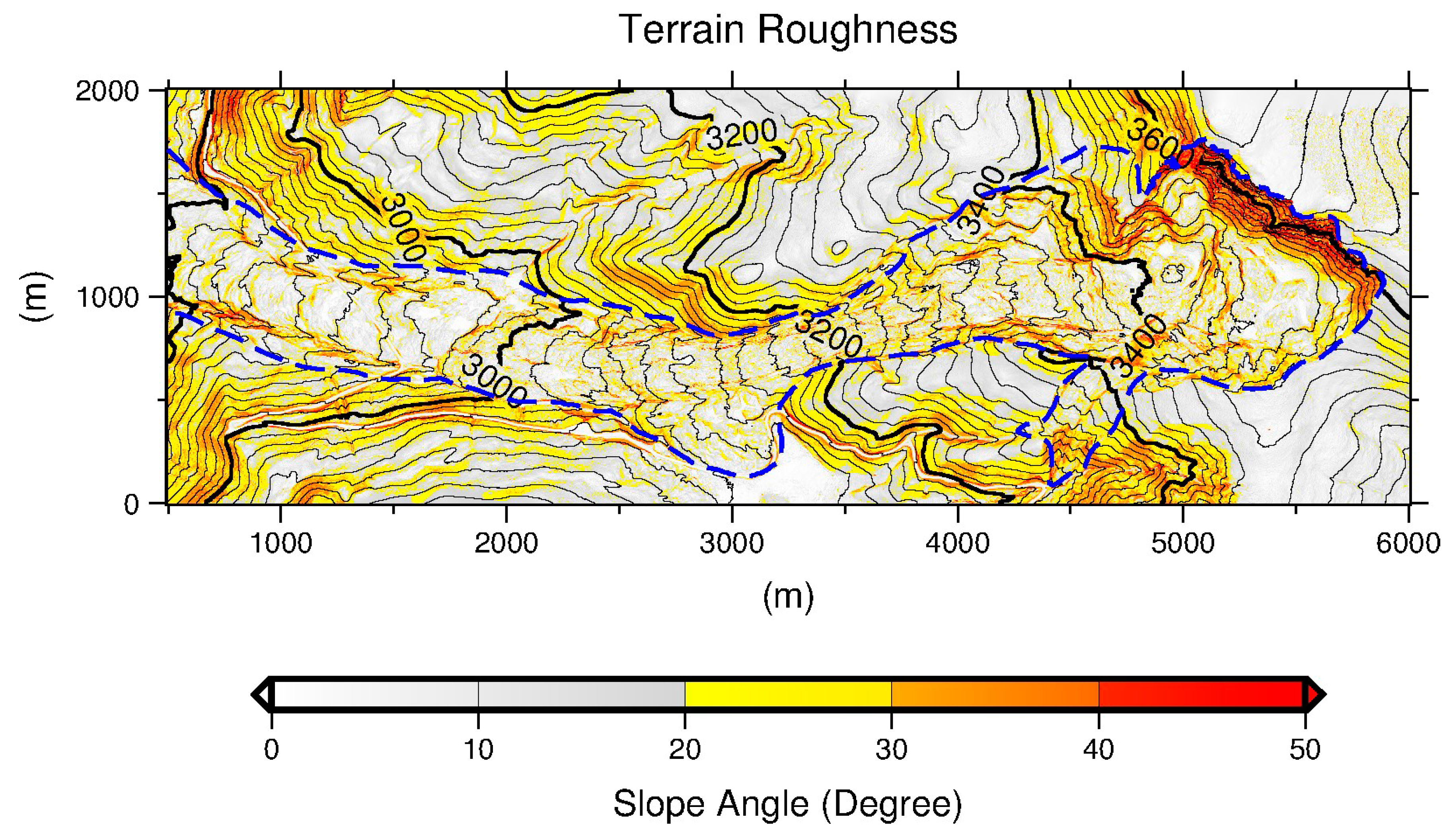
Figure 11.
Comparisons of elevation measurements derived from ALS and TLS surveys on 7 July 2015. Both ALS and TLS points have been down-sampled to 0.5-m by 0.5-m grid cells. The location of the scan area is marked in Figure 3b. (a) Elevation measurements of the bare-earth ALS points. (b) Elevation measurements of the bare-earth TLS points. (c) A shaded DEM map derived from the ALS points illustrated in (a). (d) A shaded DEM map derived from the TLS points illustrated in (b).
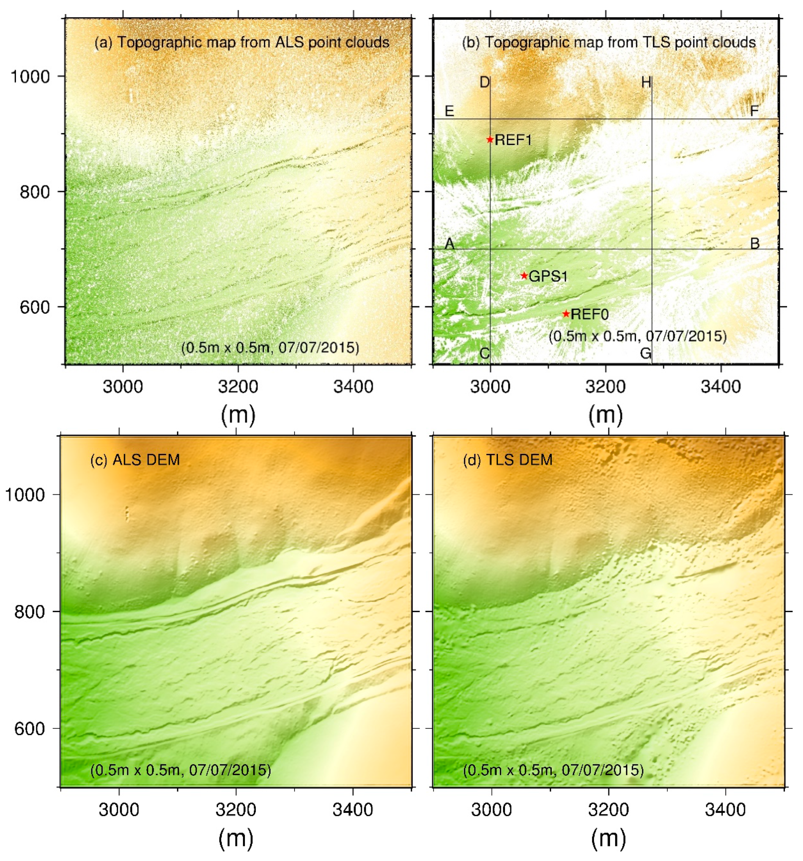
Figure 12.
Comparisons of the elevation measurements from the ALS and TLS datasets depicted in Figure 11. The left column is the elevations along profile AB; the right column is the elevations along profile CD. The root mean square of errors (RMSE) and mean values marked in subplots (e,f) are calculated from the datasets within the shaded areas where both ALS and TLS datasets have continuous data coverage.

Figure 13.
Comparisons of the elevation measurements from the ALS and TLS datasets depicted in Figure 11. The left column is for the elevations along profile EF; the right column is the elevations along profile GH. The RMSE and mean values marked in subplots are calculated from the datasets within the shaded areas that both ALS and TLS datasets have continuous data coverage.
© 2018 by the authors. Licensee MDPI, Basel, Switzerland. This article is an open access article distributed under the terms and conditions of the Creative Commons Attribution (CC BY) license (http://creativecommons.org/licenses/by/4.0/).
Share and Cite
MDPI and ACS Style
Xiong, L.; Wang, G.; Bao, Y.; Zhou, X.; Sun, X.; Zhao, R. Detectability of Repeated Airborne Laser Scanning for Mountain Landslide Monitoring. Geosciences 2018, 8, 469. https://doi.org/10.3390/geosciences8120469
AMA Style
Xiong L, Wang G, Bao Y, Zhou X, Sun X, Zhao R. Detectability of Repeated Airborne Laser Scanning for Mountain Landslide Monitoring. Geosciences. 2018; 8(12):469. https://doi.org/10.3390/geosciences8120469
Chicago/Turabian StyleXiong, Lin, Guoquan Wang, Yan Bao, Xin Zhou, Xiaohan Sun, and Ruibin Zhao. 2018. "Detectability of Repeated Airborne Laser Scanning for Mountain Landslide Monitoring" Geosciences 8, no. 12: 469. https://doi.org/10.3390/geosciences8120469
Note that from the first issue of 2016, this journal uses article numbers instead of page numbers. See further details here.