Abstract
Computation of Common Middle Point seismic sections and their subsequent time migration and diffraction imaging provides very important knowledge about the internal structure of 3D heterogeneous geological media and are key elements for successive geological interpretation. Full-scale numerical simulation, that computes all single shot seismograms, provides a full understanding of how the features of the image reflect the properties of the subsurface prototype. Unfortunately, this kind of simulations of 3D seismic surveys for realistic geological media needs huge computer resources, especially for simulation of seismic waves’ propagation through multiscale media like cavernous fractured reservoirs. Really, we need to combine smooth overburden with microstructure of reservoirs, which forces us to use locally refined grids. However, to resolve realistic statements with huge multi-shot/multi-offset acquisitions it is still not enough to provide reasonable needs of computing resources. Therefore, we propose to model 3D Common Middle Point seismic cubes directly, rather than shot-by-shot simulation with subsequent stacking. To do that we modify the well-known "exploding reflectors principle" for 3D heterogeneous multiscale media by use of the finite-difference technique on the base of grids locally refined in time and space. We develop scalable parallel software, which needs reasonable computational costs to simulate realistic models and acquisition. Numerical results for simulation of Common Middle Points sections and their time migration are presented and discussed.
1. Introduction
The major challenge in carbonates environments is how to map micro-heterogeneities, which have a significant impact on oil and gas production. In particular, in many carbonate reservoirs, matrix porosity contains the oil in place but the permeability is mainly provided by fracture corridors. In some carbonate reservoirs, the oil in place is essentially contained in karstic caves. Therefore, the ability to locate these microstructures and to characterize their properties is of a high importance. Recently various techniques to locate and characterize these structures have been developed through the analysis of scattered/diffracted elastic waves ([1]).
Traditional seismic processing and imaging are biased toward specular reflection events, and usually consider the diffractive component of the total wavefields as noise and ignore the information it contains. Any detail smaller than half the seismic wavelength cannot be interpreted in an objective, unambiguous way. Diffraction offers a different perspective on the seismic resolution. It is a reliable indicator of small structural characteristics. Also, under idealized circumstances (such as a low noise level), they allow recovery of sub-wavelength details. This makes diffractions the key to seismic super-resolution. Diffraction imaging aims to detect and delineate small-scale subsurface discontinuities and heterogeneities such as faults, unconformities, karsts, fracture swarms, buried channels etc. using seismic diffraction [1].
The first step in the development of any inversion/imaging procedure is an accurate numerical simulation of the wave field being scattered by fractures and caves. The numerical and computer constraints even on the very large clusters limit the resolution at which a model can be described. The current practice for finite-difference simulation of elastic waves propagation is to use grid cells of 0.1–0.2 of a dominant wavelength that is about 10–20 m for typical statements. Therefore, one needs to upscale heterogeneities associated with fracturing on a smaller scale (0.01–1 m), and to distribute them in an equivalent/effective medium. This effective medium will properly reproduce variations of travel-times and an average change of reflection coefficients but will absolutely cancel the scattered waves that are a subject of the recently developed methods of Diffraction/Scattering imaging for characterizing fracture distributions. The main issue with the multiscale simulation of cavernous/fractured (carbonate) reservoirs in a realistic environment is that one should take into account both macro- and microstructures, which means that the reference model will be represented with extremely excessive detailing.
From a computational point of view, this makes impossible a straightforward use of the finite difference method for modeling seismic waves’ propagation. In particular, a model of 10 km × 10 km × 10 km which is common for seismic explorations with a cell size of 0.5 m claims 8 × 10¹² cells and needs 350Tb of RAM. To overcome this issue we propose to use locally refined grids to describe small-scale heterogeneities within the target area [2]. Nevertheless, even the implementation of such adaptive grids needs significant computer resources to simulate realistic 3D seismic acquisition with thousands of sources. Therefore, we choose to simulate Common Middle Point (CMP) stack.
Common Middle Point (CMP) stack is one of the widely used approaches to time imaging of seismic data for complicated heterogeneous geological media. It brings knowledge about both geometrical (shape) and dynamical properties of the target objects and provides important input information for geological interpretation. Using the correct migration velocity, one can transfer these time sections to depth images by post-stack depth migration. Therefore, it would be very useful to compute synthetic CMP stack for realistic 3D heterogeneous media and to analyze how some specific features of the real medium, like small-scale heterogeneities (cavities, cracks and fractures and so far), are represented there.
To get this kind of synthetic 3D CMP stack for realistic multiscale heterogeneous media with reasonable computer resources we choose to supplement the use of finite-difference methods on adaptive grids with the concept of exploding reflectors (see chapter 1 of the Claerbout’s book [3] and the paper from Carcione with co-authors [4]). The basement of this choice is the common knowledge that CMP stack section computed with reasonable stacking velocities and amplitude control provides a rather good approximation of primary reflections generating by a zero-offset point-receiver acquisition, which, in turn, can be simulated on the base of exploding reflectors concept. Combination of this concept with the use of the finite-difference technique with local refinement in time and space opens the way to simulate seismic waves’ propagation through multiscale media and computation of diffraction/scattering images.
The joint use of the exploding reflectors concepts and multiscale finite-difference simulation on the base of locally refined grids for the first time opens up the possibility to simulate realistic 3D scattered/diffracted data. We use this data to validate diffraction imaging approach to detect and delineate small-scale subsurface heterogeneities. Unlike reflection, whose properties essentially depend on source-receiver separation parameter, diffraction properties are a function of the receiver distance from the diffraction object and thus, zero-offset simulation allows in practice to investigate all main features of the diffracted wavefield and diffraction imaging algorithms.
The paper has the following structure. We begin with a description of the finite-difference schemes with adaptive grids, then describe 3D realistic multiscale model (cavernous-fractured reservoir under 3D paleo-channel) and explain our approach to compute synthetic Common Middle Point Stack Sections (CMP) on the base of exploding reflectors principle. Finally, we present the method of diffraction/scattering imaging of small-scale heterogeneities with results computed for the aforementioned model. To conclude we summarize and discuss the results obtained and consider possible ways for further development.
2. Finite Difference Scheme with Locally Refined Grids
2.1. Problem Statement
As was aforementioned, the main challenge with a full-scale simulation of multiscale media like cavernous/fractured reservoirs in a realistic environment is a necessity to take into account both heterogeneities of different scales—microstructure of reservoirs and macro heterogeneities of overburden. A straightforward implementation of finite difference techniques gives an overly detailed description of the reference model. This leads to a huge amount of memory required for the simulation and, therefore, extremely high computational cost. The popular approach to reducing these demands is to refine the grid in space (see [2] for a detailed review), but it has at two main drawbacks:
- To ensure the stability of the finite-difference scheme the time step must be very small everywhere in the computational domain;
- Unreasonably small Courant ratio in the area with a coarse spatial grid leads to a noticeable increase in numerical dispersion.
Our solution is to use a mutually agreed local grid refinement in both time and space.
To construct the finite-difference we use the following velocity-stress formulation to simulate propagation of seismic waves in 3D heterogeneous media with density :
with vectors and =, describing displacement velocities and stresses within the medim. Here A, B, and C are rectangular 3 × 6 matrices with nonzero elements.
matrix D is square symmetric 6×6 with nonzero elements
where λ and μ are Lame parameters. We apply the standard second-order finite difference scheme [5], but modify its coefficients by the balance technique to guarantee the second order approximation of the elastic wave equation in heterogeneous elastic media like cavernous-fractured reservoirs. Our previous study proves this modification provides the second-order rate of convergence for reflection/transmission coefficients for solid-solid and solid-water interface with the arbitrary inclination [6]. Hence, implementation of this approach does not claim the explicit description of the solid-solid and solid-liquid interfaces, but needs in the distribution of the elastic coefficients and density on a uniform grid, which is necessary to modify coefficients of the finite-difference scheme and provide second order rate of convergence.
2.2. Formation of the Multiscale Geological Model
The approach on the base of the locally refined grids performs computations on different scales and needs the use of different seismic models: parameters of a reference medium given on a coarse grid and a detailed characterization of the immersed reservoir on a fine grid (see Figure 1). It is very important that there is absolutely no necessity to fit the interior structure of these two media—they just need to be uploaded as two different files containing the values of elastic parameters and density on two different grids. The coordinates of the opposite ends of its principal diagonal determine reservoir position. Thus, the formation of the multiscale model is to load two (or N 2, independence of the specific problem) files and the six (or 6N) digits that define the position of the target reservoir. Subdomains with both coarse and fine grids are again decomposed into elementary subdomains being assigned to individual Processor Unit (PU). Now these PU form two (or N 2) groups for grids of different scales, and special efforts should be applied in order to couple these groups.
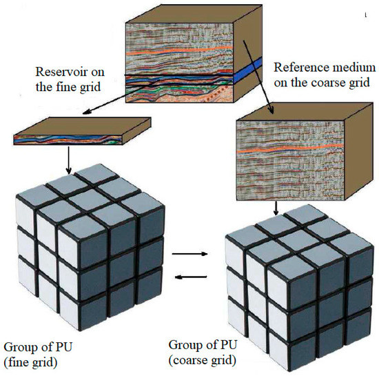
Figure 1.
Coarse—fine grid decomposition.
2.3. Coupling of Coarse and Fine Grids
Let us explain now how coarse and fine grids are coupled with each other. The necessary properties of the finite difference method based on a local grid refinement should be its stability and an acceptable level of artificial reflections. Scattered waves we are interested in have an amplitude of about 1% of the incident wave. Hence, artifacts should be at least about 0.1% of the incident wave. To achieve this level of artifacts we do the refinement in time and space by turn on two different surfaces surrounding the target area with microstructure (see Figure 2). This guarantees the stability of the finite-difference scheme and the desired level of artifacts [2].
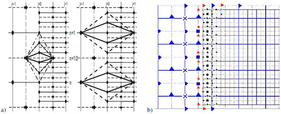
Figure 2.
The mutual disposition of fine and coarse grids. (a) In time, (b) In space.
We illustrate refinement in time with a fixed 1D spatial discretization in Figure 2a. Its modification for 2D and 3D media is straightforward (see [2] for more detail).
To refine the spatial grid, we use the Fast Fourier Transform (FFT) based interpolation. Let us explain this procedure for a 2D problem. The mutual disposition of a coarse and fine spatial grids is presented in Figure 2b), which corresponds to updating the stresses by velocities (updating velocities by stresses is implemented in the same manner). As can be seen, to update the stresses on a fine grid it is necessary to know the velocities at the points marked with small (red) triangles, which do not exist on the given coarse grid. Using the fact that all of them are on the same line (on the same plane for 3D statement), we seek the values of missing nodes by FFT based interpolation. Its main advantages are an extremely high performance and exponential accuracy. It is this accuracy allows us to provide the required low level of artifacts (about 0.001 with respect to the incident wave) generated on the interface of these two grids. For 3D statement, we again perform the FFT based interpolation but this time 2D.
2.4. Implementation of Multiscale Parallelization
Numerical simulation of seismic wave propagation in cavernous-fractured reservoirs needs parallel computations on both macro and micro scales. The simultaneous use of coarse and fine grids and the necessity of interaction between them makes it difficult to ensure a uniform load of Processor Units. Besides, the user should have the possibility to place the reservoir(s) anywhere in the background. As we already mentioned above (see Section 2.2), this problem is resolved by the use of different groups of Processor Units for different scales (Figure 3). One of them with the coarse grid is for the reference medium and the rest for a description of the reservoir. Therefore, each model scale is a set of elastic parameters and density defined on a uniform grid inside some parallelepiped and loaded as a set of corresponding binary files. Along with the loading, we perform Domain Decomposition (DD) of the current scale and assign each elementary subdomain of this DD to its individual PU. Altogether, these Processor Units form a group, which is responsible for numerical simulation on the current scale. It should be noted that this way of systematic description of multiscale media, in addition to its ease of implementation, greatly simplifies the provision of uniform loading of PU involved in computations at a different scale.
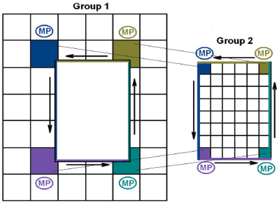
Figure 3.
Processor Units for the coarse (Left) and fine (Right) grids.
Next, we need to organize both exchanges between processes within each group and between the groups. The data exchange within a group is through the faces of the adjacent Processor Units by non-blocking iSend/iReceive procedures from the Message Passing Interface Library (MPI) in the manner explained in Section 2.2. The interaction between the groups is much more complicated. It is carried out not for data sending/receiving only, but for coupling coarse and fine grids as well.
Let us explain now how different scales are coupling with each other. For the sake of simplicity, we consider the data exchange between two groups: the first group with a coarse grid and the second one with a fine grid.
From coarse to fine: First is recovered Processor Units in the first group which surround the reservoir area, and grouped along each of the faces contacting the fine grid. At each of the faces on the coarse grids, the Master Processor (MP) is designated, which gathers the computed at this time step values of stresses/displacements and sends them to the relevant MP on the fine grid (see Figure 4). This MP provides all subsequent data processing providing the coupling of the coarse and fine grids. Later this MP sends interpolated data to each processor of the corresponding subgroup.
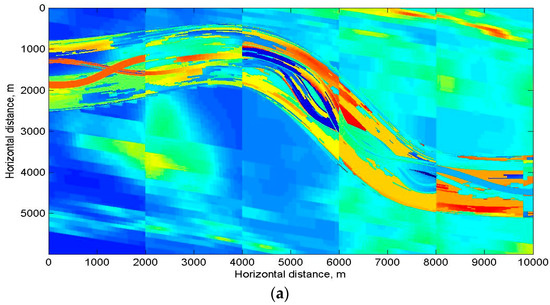
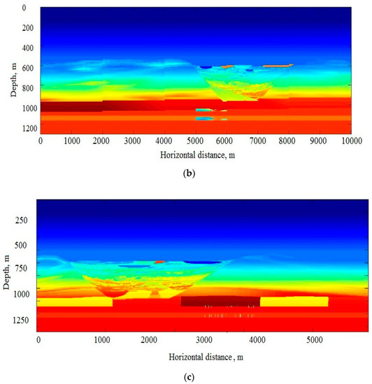
Figure 4.
3D heterogeneous multiscale geological model: paleo channel overrides fractured reservoir. (a) Horizontal cross-section at the depth 800 m, (b,c) two orthogonal vertical cross-sections through the middle of the model.
The choice to carry out interpolation by the MP of the second group essentially decreases the amount of sent/received data and, hence, the waiting (idle) time of processor units.
From fine to coarse.: As in the previous case, primarily we identify PU from the second group which performs computations on the faces covering the area with the fine grid. Next, again for each face is set up a Master Processor. This MP as its partner from the coarse grid collects data from the relevant face of the reservoir and performs their preprocessing before sending to the first group of PU (a coarse grid). Now we do not need all data in order to move to the next time, but only those of them, which fit the coarse grid. Formally, these data could be obtained by thinning out the fine grid, but our numerical experiments have proved that this way generates significant artifacts due to the loss of smoothness. Therefore, for this direction (from fine to coarse) we also use the FFT based interpolation implemented by the relevant MP of the second group (a fine grid). The data obtained are sent to the first group.
3. The Multiscale Model Used for Validation of the Method
To validate the approach for CMP computations via exploding reflectors concept and subsequent use of synthetic CMP for scattering imaging, we choose the multiscale model presented in Figure 4. This model describes some realistic 3D heterogeneous multiscale geological medium—a carbonate reservoir with fracture corridors imbedded under paleo-channel. The macroscale referent medium is made of a thick sub-horizontal layers with curvilinear heterogeneous paleo-channel. The 3D heterogeneous carbonate reservoir with fracture corridors can be seen under this macroscale overburden (see Figure 4).
This reservoir is the horizontal layer of 200 m thick and has two constituents: rock matrix and fracture corridors within this matrix. The rock matrix parameters are: , , density . It contains two layers of 30m thick each with fracture corridors (Figure 5. Fracture corridors are parallel randomly distributed within each layer. Each fracture corridor is given by a grid of 30 m × 1000 m × 50 m size with cells as small as 0.5 m × 0.5 m × 0.5 m (Figure 5d). The fracture density varies from zero in the non-fractured facies to maximal value equal to 0.3. Finally, we transform the fracture density to elastic parameters using the second order Hudson theory [7]. We fill fractures with gas, which diminishes the velocity down to 3600m/s the lowermost as compared to 4400 m/s in the matrix.
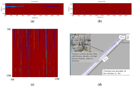
Figure 5.
Sketch of the reservoir. (a–c)—side and top views. (d) Upscaling of the fractures to fracture corridors.
4. Exploding Reflectors
Common Middle Point (CMP) stack section does not only transform multi-shot multi-offset seismic data to zero-offset data but also significantly reduces the multiples. In order to imitate this procedure, we need to apply some special smoothing of the background together with forming the so-called secondary sources. One must keep in the mind when implementing exploding reflectors two main features:
- The macro-velocity model should be reasonably smooth to produce significant reflections, but barely change global travel times;
- The secondary sources should possess proper intensity in order to generate reflected/scattered waves with correct amplitudes.
4.1. Smoothing of the Full Model
To provide the desired features of the model we need to keep in the mind the principal property of the propagator—it should not produce any significant, but save up to reasonable accuracy “global” travel times, in particular times from acquisition to target objects and backward. To guarantee these properties we use smoothing on the base of the Error Function [8]:
Smoothing of a function f(z) is done by means of its convolution with Gaussian kernel:
The detailed explanation of how to choose parameters α and we give in Appendix A.
We smooth the P- and S-slowness at each point x with respect to z. In Figure 6a,b we present the central vertical cross-section of the full initial model and its smoothed version.
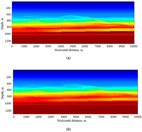
Figure 6.
The vertical cross-section of the paleo-channel model. (a) No smoothing (b) After smoothing.
Let us estimate the quality of the smoothing and start with the reflectivity, which we treat as a reflection coefficient for a normally incident plane wave:
In Figure 7a,b we compare reflectivity and travel-times for the models before and after smoothing. As one can see, the reflectivity after smoothing is negligible in comparison with its initial distribution, and the travel time perturbations do not exceed 1 ms.
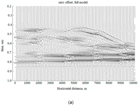
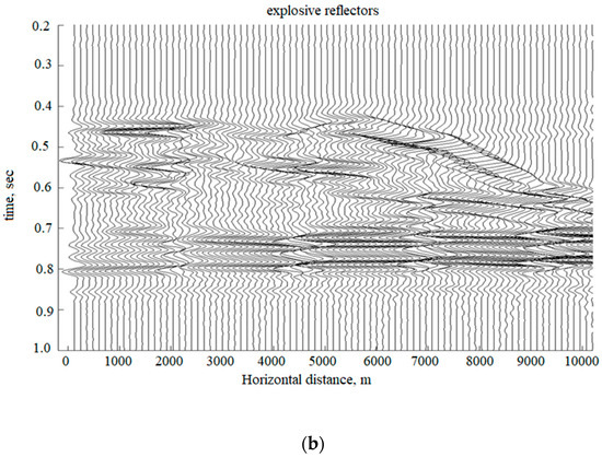
Figure 7.
Comparison of zero offset 2D seismogram computed for the full model (a) and the one computed by exploding reflectors technique, presented in Section 4 (b).
4.2. Secondary Sources
Here we derive new formulas to reformulate statement with a point source to the exploding reflectors. Let us analyze now the secondary sources, produced by propagator perturbations. To do that we consider the medium as a superposition of smooth propagator and its sharp perturbations, which we call a reflector:
The solution of the elastic wave equation we decompose in the same manner:
This leads to the following system of partial differential equations for wave’s propagation from volumetric point source:
From this point on, for us is more convenient to use the system of partial differential equations of the second order for displacement. The regularity of the forward map is well studied [9] and under some natural conditions, in particular, smoothness of the source function , the linearization procedure is correct and gives the following system of partial differential equations:
For the incident wavefield , propagating in the smooth background (propagator)
Operators and are given as follows:
For the reflected/diffracted/scattered wavefield :
with the same differential operators and , and new differential operators and given by:
To close (1) and (2) we add zero initial conditions:
In the time-frequency domain Equation (2) can be rewritten as:
A solution of this equation has the following integral representation:
with Green’s matrix .
In a smooth background/propagator volumetric source generates mainly P-wave in the following form [10]:
where is Fourier spectrum of the source function , is the amplitude of the incident wave, —travel-time from the source to the observation point and —polarization vector. Straightforward computations (see Appendix B) give the following equation for the backscattered wavefield for zero offset observations:
Let us remind, that is perturbation of the Lame parameter .
4.3. Numerical Experiments
To validate the results we present the results of the 2D numerical simulation. We compare zero offset seismogram computed for the full model presented in Figure 6a and exploded reflectors seismogram computed following the approach presented before: we do the smoothing of the model (see propagator in the Figure 6b) and compute the secondary source. These results one can see in the Figure 7a,b.
As one can see, there is no visible difference between two these seismograms, therefore to see that they do not coincide each other we present the zoomed version of some trace, computed by these methods in Figure 8. As one can see, there are really non-significant differences in arrival times and amplitudes of a few events.
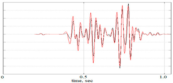
Figure 8.
Comparison of a zero offset trace, computed by full finite difference simulation (black) and exploding reflectors approach (red).
5. Diffraction Imaging
The exploding reflector scheme described above was used in order to compute the full 3D zero-offset cube for the model presented in Figure 4. In order to accurately account for small-scale reservoir elements such as fractures, local grid refinement in time and space is used within the finite-difference scheme. Figure 9 shows the general view of the computed cube. Main reflection events are clearly visible. Small-scale elements of the channel and numerous fractures give raise to seismic diffraction. It is worth mentioning that implementation of exploding reflectors scheme claims reasonable computer resources: it took 8 h on 240 cores computer.
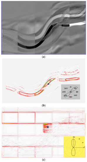
Figure 9.
(a) Poststack time migration image at t = 0.5 s. (b) Poststack time domain diffraction image at t = 0.5 s. (c) Poststack time domain diffraction image at t = 0.84 s.
In the Figure 10, we represent the 3D view of the regular time migration image (both reflection and diffraction) computed for exploding reflectors approximation.
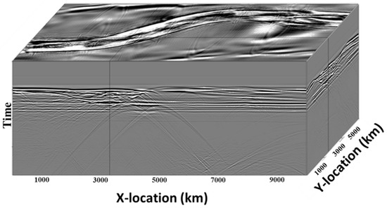
Figure 10.
Zero-offset cube computed by the adaptive FD scheme for the model shown in Figure 5.
For diffraction imaging, we used popular today the so-called dip angle common image gathers (CIG) which are computed in the reference system of the model domain [11]. In this coordinates there is a significant difference in the behavior of reflected and diffracted waves and this difference can be used for their separation [12]. In [11,13] they offered a separation and diffraction imaging method based on separation and migration. For full azimuth observations, azimuthal dependence of diffraction can be used to estimate fracture orientation [1].
We applied dip-angle based separation procedure to the computed data сube and then depth migrated the diffractive component only. Resulting diffraction imaging cube contains mostly focused diffraction energy and can be interpreted together with a standard structural cube to improve the reliability of interpretation of discontinuities and other small scale subsurface elements including fracture corridors. Figure 9 compares time sections at t = 0.5 s:
- (a)
- poststack time migration (PSTM);
- (b)
- time domain diffraction section.
At the Figure 9b (right bottom corner) we show the so-called diffraction rose-diagram for a point marked by a star on the diffraction image. The rose diagram determines the direction of maximal diffraction energy corresponding to the tangent to the channel and, hence, indicating the “edge diffraction” [14].
The next diffraction image (Figure 9c) corresponds to the time slice of t = 0.84 s. As one can see how the propagation of the maximal diffraction energy (see rose diagram in the right bottom corner of the figure) corresponds to the orientation of fracture corridors. The most reliable explanation of this fact is the heterogeneous interior structure of each corridor. As one can see in Figure 5, the interior of these corridors is highly irregular and therefore generates intensive diffraction. In other words, we observe two different types of diffraction—the first is generated mainly by the sharp edges of the paleochannel (Figure 9b), while the main source of the second (Figure 9c) is interior heterogeneity of the fracture corridors. Strictly speaking, it would be more correct, to associate the second case not with diffraction, but with scattering by the conglomerates of small-scale heterogeneities.
6. Discussion
This work combines two at the first glance different statements
- numerical simulation of seismic wave propagation in three-dimensional inhomogeneous multi-scale media;
- imaging of small-scale inhomogeneities by focusing the energy of diffracted/scattered waves.
However, in reality, these two tasks are very close to each other. Indeed, any imaging procedure requires its verification on a fairly complex, maximally realistic model. This requires synthetic wave fields, which will be used to build images. At the same time, the straightforward application of finite-difference methods for solving such a problem in the full statement of multi-shot multi-offset acquisition leads to the need to use an excessively small step and, consequently, to unrealistic requirements for the RAM and performance of the computing systems used.
We could avoid such excessive computers demands due to two factors:
- Use of grids with local grinding of a step in time and space;
- Modeling post stack seismic wave fields directly by applying exploded reflectors concept.
It should be noted that post stack data are widely used in the seismic analysis and occupy an important place processing and interpretation for studying the features of the geological structure. Undoubtedly, the advantage of this representation of the wave field is its rather small computer memory needed compared with the prestack data volume. At the same time, the main features of the geological structure, including the presence of small-scale inhomogeneities, manifest them very clearly, which is confirmed by the obtained results of diffraction imaging.
To stress the significance of the results obtained let us draw attention to the difference in diffraction images computed at the level of the paleochannel and at the level of the fractured reservoir. The main direction of diffracted energy propagation at the paleochannel level is oriented along the tangent to the coast line, which we associate with the appearance of the edge wave [14]. At the same time, at the reservoir level, the diffracted energy spreads both along and across the cracks. In our opinion, this is due to the fact that the cracks are not ideal parallelepipeds with smooth faces and edges, but are filled with small-scale inhomogeneities. Each of them is the object of diffraction\scattering, generating intense diffracted\scattered waves.
Thus, we can assert that cracks filled with geological rocks containing small-scale heterogeneities (for example, tectonic breccias) will generate diffracted\scattered waves propagating in different directions. These directions are governed by the size and orientation of the above-mentioned small-scale inhomogeneities. In this sense, the fundamental difference between diffracted\scattered waves formed at the edges of the paleochannel and interacting with tectonic cracks lies precisely in the objects generating them—the relatively smooth shores of the paleochannels and sharply changing in space small-scale inhomogeneities filling the cracks.
Here we would like to pay the special attention to the advantages we gain by using finite-difference schemes with local grid refinement in time and space. Of course, our approach to do that is not unique—there are various approaches, especially in computer fluid dynamics (see, e.g., [15]). However, in our opinion, the problem we deal with in seismic simulation is specific—the medium does not change in time and we do not need to change the grid from one time step to another. Hence, we can fix the grid and use the same refinement. Moreover, we never know the exact shape of microheterogeneities, and, hence, do not need to fit the grid with them. Therefore, we choose to use the usual Cartesian grid. Next, our approach aims to deal with sub-horizontal reservoirs, which can be placed within thin parallelepiped. Hence, the user needs to point out coordinates of the main diagonal of this parallelepiped and software will do refinement exactly within. This essentially facilitates preparation of the model and the way to implement computations.
7. Conclusions
To conclude, let us underline that in the paper we develop the closed cycle of mathematical simulation, which provides solution of the both direct and inverse problems of waves’ propagation in multiscale 3D heterogeneous elastic media. We did very interesting and important observation by the different nature of diffraction on the ancient coastline of the paleo channel and scattering by the small-scale heterogeneities within fracture corridors.
We see the following directions of the further development of the technique presented above:
- non-zero offset;
- viscoelastic media;
- anisotropic and visco anisotropic media.
Author Contributions
E.L. proposes the concept of application of exploding reflectors to the diffraction imaging. He also developed and implemented the diffraction imaging procedure for poststack 3D seismic data. V.T. derived the equations for exploding reflectors in multiscale elastic media. He proposed and validated the rule of construction of the correct secondary sources, providing the desired wavefield. G.R. proposed the algorithm of elastic wave simulation in multiscale media on the base of locally refined grids and developed corresponding parallel software.
Funding
Galina Reshetova and Vladimir Tcheverda have been supported by the Russian Science Foundation, project 17-17-01128.
Acknowledgments
We thank two anonymous reviewers for their careful reading of the manuscript and friendly and helpful remarks and comments.
Conflicts of Interest
The authors declare no conflict of interest.
Appendix A
The error function, also known as the Gauss error function, is a special function defined as [8]:
This function has a sigmoid shape and is analytical (Figure A1).

Figure A1.
Error function.
Smoothing of any function is done by means of its convolution with error funcion:
We need to smooth a model in a manner reducing reflections, but not perturbing travel times to some extent. In order to guarantee the last property let us search for parameters of transformation (4) saving constantly ith given accuracy:
In our considerations we choose , so and any constant after smoothing saves its value with single computer precision.
In particular, let us consider what happens with a piece-wise constant model being piece-wise constant with respect to :
Then the smoothed model for is equal to or respectively with single computer precision , while within (0,H) it looks like:
Appendix B
As we proved already in the Section 4.2 the scattered wavefield has the following integral representation (see Equation (A1)):
with Green’s matrix . As we mentioned in the same section in a smooth background/propagator volumetric source generates mainly P-wave in the following form:
where is Fourier spectrum of the source function , is the amplitude of the incident wave, —travel-time from the source to the observation point and —polarization vector. Let us suppose now that support of some specific perturbation is rather small so that the medium inside may be treated as homogeneous and is its “middle” point where would be assigned values of all variables. In particular, within this interior the incident wave can be written down as the following plane wave:
For the sake of simplicity we introduce a local Cartesian coordinates with parallel to and come to the following formulaes within support of perturbations of material parameters:
and the second term in the right hand side of definition ( ) can be written down as the vector
Finally we come to the following representation of the “secondary” sources:
We will assume that is supported in a small ball with center at and turns to zero on the . Then on the base of Gauss identity:
the formula (5) for a scattered wavefield can be rewritten as:
Therefore this wavefield can be treated as generated by the elementary secondary volumetric source, that is as a solution to the following equation:
Again, for rather smooth background/propagator we come to the representation of scattered wavefield
which for zero offset transforms to
and, taking into account reciprocity for travel-times and amplitudes, we have the following representation of zero-offset wavefield:
After introducing new time frequency this formula can be rewritten as
This relation proves that wavefield being generated by the source at and back scattered by the point scatterer at , can be treated as a solution to the following equation:
that is created by a secondary volumetric source at and amplitude , where is amplitude of the incident wave from the volumetric point source at .
References
- Landa, E. Seismic diffraction: Where’s the value? In Proceedings of the 2012 SEG Annual Meeting, Las Vegas, NV, USA, 4–9 November 2012; Society of Exploration Geophysicists: Houston, TX, USA, 2012. SEG-2012-1602. [Google Scholar]
- Lisitsa, V.; Reshetova, G.; Tcheverda, V. Finite-difference algorithms with local time-space grid refinement for simulation of waves. Comput. Geosci. 2012, 16, 39–54. [Google Scholar] [CrossRef]
- Claerbout, J. Introduction to imaging. In Imaging the Erath’s Interior; ACM Digital Library: Oxford, UK, 1985; pp. 1–13. ISBN 0-86542-304-0. [Google Scholar]
- Carcione, J.M.; Boehm, G.; Marchetti, A. Simulation of CMP seismic sections. J. Seism. Explor. 1994, 3, 381–396. [Google Scholar]
- Virieux, J. P-SV wave propagation in heterogeneous media: Velocity-stress finite difference method. Geophysics 1986, 51, 889–901. [Google Scholar] [CrossRef]
- Vishnevsky, D.; Lisitsa, V.; Tcheverda, V.; Reshetova, G. Numerical study of the interface errors of finite-difference simulations of seismic waves. Geophysics 2014, 79, T219–T232. [Google Scholar] [CrossRef]
- Mavko, G.; Mukerji, T.; Dvorkin, J. Rock Physics Handbook; Cambridge University Press: Cambridge, UK, 2009; pp. 266–346. ISBN 10: 0521861365. [Google Scholar]
- Cody, W.J. Rational chebyshev approximation for the error function. Math. Comput. 1969, 23, 631–638. [Google Scholar] [CrossRef]
- Bao, G.; Symes, W. Regularity of an inverse problem in wave propagation. Lect. Notes Phys. 1997, 486, 226–235. [Google Scholar]
- Červený, V. Seismic rays and travel times. In Seismic Ray Theory; Cambridge University Press: Cambridge, UK, 2001; pp. 99–233. [Google Scholar]
- Landa, E.; Fomel, S.; Reshef, M. Separation, Imaging, and Velocity Analysis of Seismic Diffractions Using Migrated Dip-Angle Gathers; Extended Abstract; SEG: Las Vegas, NV, USA, 2008; pp. 2176–2180. [Google Scholar]
- Reshef, M.; Landa, E. Post-stack velocity analysis in the dip-angle domain using diffractions. Geophys. Prospect. 2009, 57, 811–821. [Google Scholar] [CrossRef]
- Klokov, A.; Baina, R.; Landa, E. Separation and Imaging of Seismic Diffractions in Dip Angle Domain; Extended Abstract; EAGE: Barcelona, Spain, 2010. [Google Scholar]
- Keller, J.B. Geometrical theory of diffraction. J. Opt. Soc. Am. 1952, 52, 116–130. [Google Scholar] [CrossRef]
- Mao, S. A new hybrid adaptive mesh algorithm based on Voronoi tessellations and equi-distribution principle: Algorithms and numerical experiments. Comput. Fluids 2015, 109, 137–154. [Google Scholar] [CrossRef]
© 2018 by the authors. Licensee MDPI, Basel, Switzerland. This article is an open access article distributed under the terms and conditions of the Creative Commons Attribution (CC BY) license (http://creativecommons.org/licenses/by/4.0/).