Generating Observation-Based Snow Depletion Curves for Use in Snow Cover Data Assimilation


1
SAIC, Inc., McLean, VA 22101, USA
2
Department of Geography and Geoinformation Science, George Mason University, Fairfax, VA 22030, USA
*
Author to whom correspondence should be addressed.
Geosciences 2018, 8(12), 484; https://doi.org/10.3390/geosciences8120484
Submission received: 1 November 2018
/
Revised: 6 December 2018
/
Accepted: 10 December 2018
/
Published: 14 December 2018
(This article belongs to the Special Issue Remote Sensing of Snow and Its Applications)
Abstract
:Snow depletion curves (SDC) are functions that are used to show the relationship between snow covered area and snow depth or water equivalent. Previous snow cover data assimilation (DA) studies have used theoretical SDC models as observation operators to map snow depth to snow cover fraction (SCF). In this study, a new approach is introduced that uses snow water equivalent (SWE) observations and satellite-based SCF retrievals to derive SDC relationships for use in an Ensemble Kalman filter (EnKF) to assimilate snow cover estimates. A histogram analysis is used to bin the SWE observations, which the corresponding SCF observations are then averaged within, helping to constrain the amount of data dispersion across different temporal and regional conditions. Logarithmic functions are linearly regressed with the binned average values, for two U.S. mountainous states: Colorado and Washington. The SDC-based logarithmic functions are used as EnKF observation operators, and the satellite-based SCF estimates are assimilated into a land surface model. Assimilating satellite-based SCF estimates with the observation-based SDC shows a reduction in SWE-related RMSE values compared to the model-based SDC functions. In addition, observation-based SDC functions were derived for different intra-annual and physiographic conditions, and landcover and elevation bands. Lower SWE-based RMSE values are also found with many of these categorical observation-based SDC EnKF experiments. All assimilation experiments perform better than the open-loop runs, except for the Washington region’s 2004–2005 snow season, which was a major drought year that was difficult to capture with the ensembles and observations.
1. Introduction
Snow depletion curves (SDC) define the relationship between changes in snow cover area (SCA) and the snow pack, which can impact, for example, snow-albedo feedback in global climate models [1] and the amount of water storage and melt for hydrological models [2,3]. SDCs typically involve functions that are fit or tuned to a given set of snow-based observations or theoretical conditions. Currently, many hydrological, land surface models (LSMs), and climate models use simple to complex schemes to define this snow depth-cover relationship, with many models still using very simple schemes, which do not account for even regional or temporal changes [4]. Some approaches to estimating snow depth-snow cover relationships involve statistical approaches, from using simple fitted functions to more shape and scale parameter-based gamma and beta distributions [4,5,6,7,8]. Much of the snowpack depletion in mountainous regions relates to late winter and early spring peak snow water equivalent (SWE) melt energy and radiation spatial variations (e.g., [2,9]), even though SWE can decrease without decreasing areal snow cover.
Several SDC schemes have been used to map the predicted SWE or snow depth states to snow cover fraction (SCF) (or vice versa) for different snow cover data assimilation (DA) approaches [10,11,12]. The SDC scheme can be used as the observation operator, which relates the model variables to the observations. In this case, the SDC acts as the observation operator and converts snow-based model estimates (e.g., SWE) to be in the same units and similar value range as the snow cover observation estimates (e.g., snow cover fraction), for calculating the innovation and assimilation update. The innovation step is simply the difference taken between model-generated snow cover and the observed snow cover estimates. Some studies have utilized the Ensemble Kalman Filter (EnKF) to assimilate snow cover fraction or area observations [10,13,14], as it has been shown to perform overall better than simpler methods, e.g., direct insertion [15]. EnKF relies on an ensemble of model forecasts generated using error covariances. Snow cover assimilation using the EnKF method has been applied at different scales, including global [16], continental [13], and regional [10,14,15,17]. Other ensemble-based snow cover DA studies have used the ensemble square-root filter [18] and the particle filter [19].
A variety of SDC functions have been used as the observation operator in these past snow-cover DA studies. Cumulative density functions (CDFs) of beta distributions for varying conditions have been applied regionally [10], or tuning of a hyperbolic tangent formulation, using shape parameters and a snow density parameter [20], has been applied also for different scales [13,16]. Other studies have used, for example, a two-parameter based lognormal probability distribution function, where snow cover area was represented as a summation of areal SWE and the SDCs were tuned by varying different coefficient of variation (CV) parameters for melt and accumulation periods [18]. Such SDC-based observation operator schemes have accounted for varying conditions, such as elevation, vegetation and accumulation and ablation phases [10,13,17]. Accounting for the accumulation and ablation phases, also referred to as the hysteresis characteristic of snow, can be a very important aspect of the SDC scheme, since different curves can represent these phases and are reflected in the curve parameters (e.g., [10,17]).
Previous studies that have assimilated satellite-based snow cover to improve model snow states and other hydrological variables (e.g., streamflow) have utilized snow observations to tune the snow depletion curves. Despite these previous efforts, many of the SDCs used in snow cover assimilation may have been considered theoretically simplistic [12,14] or tuned with very coarse spatial scale snow observations [20], and these SDCs may not be suitable enough for assimilating snow cover data for finer scale, mountainous regions. Also, what if the snow observations themselves were used to derive the snow depletion curves to be used as the observation operators for snow cover assimilation? One recent study used satellite-based snow cover and five snow depth stations to derive SDC functions, based on the hyperbolic tangent formulation, to derive such observation operators for a mountainous catchment in China [17]. Xu et al. [17] generated curves separately for each station and the two snow phases, accumulation and ablation. Assimilating snow cover into an LSM using these highly tuned observational based observation operators improved the modeled snow depth states at those few sites [17]. Another recent study, which focused on generating SDCs at different scales by using observed SWE and satellite-based snow cover area, showed how using such observational information can help estimate better SWE conditions (e.g., peak SWE) when 100% snow cover occurs (for an area or grid cell), given the location or area being represented [2].
In this study, we present a new approach to estimating snow depletion curves and their application for assimilating snow cover fraction observations, using an EnKF data assimilation approach and a land surface model with a multi-layer snow physics scheme. Building upon these recent studies, we use observed SWE and snow cover fraction estimates to derive new SDCs, using a larger array of observations, spanning two different mountainous regions in the United States (U.S.). We refer to these new SDC-type observation operators as “observation-based” and benchmark their skill against the default, model-based SDC function. These new SDC observation-based observation operators are hypothesized to improve the model-based SCF forecasts and snow state analysis. A secondary goal in applying this SDC approach is to see how accounting for varying vegetation, elevation, and temporal conditions may better capture heterogeneous features related to the snowpack and snow cover patterns when assimilating snow cover observations. Finally, the new SDC-based observation operators are used to derive the observational errors, which are used in the EnKF method. Accounting for different errors related to the varying conditions provides different weighting of the snow cover observations against that of the model in the EnKF innovation and update steps.
The primary research question is: How do these new observation-based, SDC-type operational operators perform relative to a default model-based scheme when assimilating snow cover estimates? The secondary research question is: How does accounting for different temporal and physiographic conditions in relation to the new observation-based SDC impact the assimilation of the snow cover estimates? We address these questions throughout the paper within the following sections. Section 2 provides an overview of the study regions, and Section 3 provides several details of the snow observations, the multi-layer snow model, and data assimilation method used in this study. Section 4 describes the method on how the new observation-based SDCs are derived and applied in the EnKF assimilation approach, and Section 5 presents the results of the new SDCs applied as the observation operator when assimilating the snow cover observations. Finally, we discuss the results, benefits and challenges of this new SDC approach in the Discussion and Conclusions section.
2. Study Area
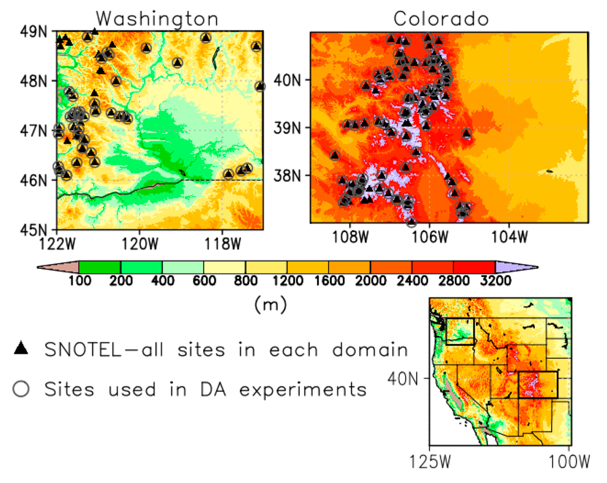
The study domains span the mountainous regions of Washington (WA) and Colorado (CO) states within the United States. The spatial grid is on an equirectangular projection with a resolution of 0.01 degree (~1 km) with bounding coordinates of the lower left corner (45.005° N, −121.995° W) and upper right corner (48.995° N, −116.995° W) for WA (400 latitudinal and 501 longitudinal points), and lower left corner (37.005° N, −108.995° W) and upper right corner (40.995° N, −102.005° W) for CO (400 latitudinal and 700 longitudinal points). The 0.01° gridcells are represented at the center of the gridcell, as reflected in the bounding coordinates. Figure 1 highlights the WA and CO study areas, depicting the areas’ high topographic variability (e.g., mountainous and low-land areas). The 0.01° elevation maps are derived from the 30 m U.S. Geological Survey (USGS) National Elevation Dataset (NED; https://lta.cr.usgs.gov/NED). Also, these areas have a wide range of soil and vegetation types (e.g., coniferous forests, grasslands, agricultural, etc.). The regions were selected to capture not only the topographic variability, but also variability in surface snow amounts. Figure 1 also shows each region’s associated in-situ U.S. Department of Agriculture’s (USDA) Natural Resources Conservation Service (NRCS) SNOwpack TELemetry (SNOTEL) measurement networks used in this study. After additional quality-control checks, 56 SNOTEL stations are identified as being within the WA domain, and 98 SNOTEL stations are within the CO domain (represented by black triangles). These stations are used in deriving and the new SDCs, as described in Section 4.1.
3. Data and Model Sources
3.1. Observational Datasets Used
The Terra MODIS Level 3, collection 5 (MOD10A1), daily 500 m snow cover fraction (SCF) product has been selected for the work presented here [21,22]. This product is derived from the MODIS Normalized Difference Snow Index (NDSI) to estimate an SCF value for each 500 m pixel [21,23]) The MODIS snow cover products are obtained from the National Snow and Ice Data Center (NSIDC) in Boulder, Colorado, USA (http://nsidc.org/data/mod10a1) [24]. The 500 m MODIS snow cover estimates have been shown to be sufficient in high mountain terrain [25]. The daily 500 m products come in a sinusoidal projection, which are resampled with the nearest neighbor using the MODIS Reprojection Tool [26] to a 0.01° geographic coordinate system (GCS) for our model and DA experiments. The original 500 m sinusoidal projection dataset is used for deriving the observation-based SDCs and observational errors, which are further described in Section 4.
The main SWE observation dataset used in this study is the SNOTEL network dataset [27]. The daily SNOTEL SWE measurements are observed using snow pillow instruments. The SNOTEL network is sometimes one of the only datasets available in mountainous areas in the U.S. to validate model estimates [28], which provide important information, like streamflow, in key water supply areas in the mountainous West [29]. The SNOTEL data used in this study include Water Years 2000–2010, which overlap the Terra/MODIS data period selected. Note: A water year (WY) is used in many hydrological studies and starts on October 1 and goes to September 30 of the following year, spanning one full snow season cycle. The SNOTEL stations are point measurements, but applied here as a representative over the gridcell (e.g., 0.01° cells). New SDCs are derived from the above MODIS SCF and SNOTEL SWE observations (which is further described in Section 4).
3.2. Land Surface Model Description and Setup
The LSM used in this study is the Community Land Model, version 2.0 (CLM2) [30,31,32]. CLM2 is run in an off-line mode, uncoupled to any atmospheric or other modeling component, and driven within the Land Information System (LIS) framework [33]. The use of LIS allows us to take advantage of its many DA, observational, and model interface capabilities. At the time of this study, later versions of CLM were not available in LIS though CLM2 was already implemented and well tested. The model contains ten soil layers with varying thickness, and a five-layer snow scheme, which accounts for liquid, ice, and heat energy storages and changes within each layer. The water balance equations are mass conserving with inputs provided mainly by precipitation and outputs associated through evapotranspiration sources (e.g., vegetation and soil) and runoff. The snow parameterizations are adapted mostly from other studies [34,35,36]. The snow scheme’s layers can grow and collapse, with the number of layers and a layer’s thickness being dependent on snow depth. Any solid precipitation (i.e., snowfall) is automatically integrated with surface snow or soil layers, and any rainfall is incorporated after fluxes and temperatures are updated [32].
Snow cover fraction affects surface albedo, net shortwave radiation, and almost all subsequent model energy and temperature calculations. Despite being such an important model component, it is parameterized in CLM2 and other LSMs as a predicted variable, dependent mainly on total snow depth (m). Therefore, any knowledge of snow cover from the previous timestep is only retained via the depth of the snowpack. CLM2’s SCF calculation employs a single, nonlinear formula that is a function of both the snow depth state and momentum of roughness parameter (m) for soil, which is set to a default value of 0.01 m. The snow fraction value is then used in the overall direct and diffuse beam ground albedo calculations and subsequent energy and moisture flux predictions. Comparison studies have shown CLM2 to perform well in different regions and settings, especially for snow [31,37,38]. Subsequent versions of CLM (3.5 and greater) have incorporated additional updates to the snow physics with varying improvement (e.g., [20,39]) and will be made available in future releases of LIS.
The meteorological forcing dataset used to drive the CLM2 simulations is from the North American Land Data Assimilation System (NLDAS) [40]. The University of Maryland (UMD) land classification dataset, derived from the Terra MODIS (collection 4) UMD land cover classification product is used [41]. The CLM2’s plant function type classification scheme and parameters were mapped to the UMD classification. For the elevation map, the 1 km NED elevation dataset is used. For further details of the CLM2 model set up and its use for this study, please see Arsenault et al. [15].
3.3. Data Assimilation Method and Experiment Setup
To assimilate the MODIS snow cover fraction estimates into CLM2, the 1-D Ensemble Kalman Filter (EnKF) method is used in this study, as adapted from Reichle et al. [42,43], which is also part of the LIS DA framework [44]. The SWE and snow depth states are perturbed, along with forcing fields that more effectively drive snow dynamics (e.g., precipitation, shortwave radiation), to generate the ensemble of model forecast conditions with 12 members. The DA methods and parameters used in this study are further outlined and described in De Lannoy et al. [14] and Arsenault et al. [15]. The MODIS SCF observations are also perturbed, as done with the EnKF method. The Terra MODIS SCF product is assimilated into CLM2 close to its local overpass time near 10:00 am local overpass time. Additional details of the snow cover assimilation, observation operators, and observation errors are further described in Section 4 and Section 5.
An open-loop (OL) simulation was generated, which is a baseline simulation where no observations are assimilated, and is used as the benchmark experiment to compare the assimilated runs against. The CLM2 OL and DA experiments include a spin-up time period from 30 September 1999, to 30 September 2003. For the OL and DA experiments, a slightly smaller number of stations were used, since CLM2 was found to build “glacier-like” points (i.e., snowpack does not completely melt off during the summer months), due to (1) a cold-bias in the NLDAS temperature field, especially when brought to finer elevation scales (e.g., 1 KM); and (2) an absence of blowing snow represented in the model, which can be a major snow removal process near mountain terrain peaks [45]. Eliminating these “glacier” type points from the DA and analysis restricts the evaluation of the new SDC-based observation operators to the more normally varying snow accumulation and melt grid points. The reduction in stations resulted in a final 40 stations for WA and 78 for CO, versus the original 56 and 98, respectively, used in deriving the observation-based SDCs. These final stations and corresponding gridcells are highlighted with open grey circles in Figure 1, and they are used for the DA experiments and statistical results, shown in Section 5.
4. Methods
4.1. Deriving the Snow Depletion Curves from Snow Observations
To help capture the range of observed SWE and SCF relationships, a histogram analysis is introduced that allows for reducing the dispersion of data and retaining most measurements within the analysis. A binned scatterplot method is used where SNOTEL SWE observations (along the x-axis) are grouped in to bins of equal length (e.g., 40 mm of SWE) and the corresponding MODIS SCF observations are averaged within the given bin. This approach allows for highlighting relationships that may otherwise be masked in a normal scatter plot (e.g., [46,47]). For each bin, a boxplot can be produced to reflect the spread in MODIS SCF values for that given bin and be represented by that bin’s statistics (mean, median, minimum/maximum, etc.). Figure 2 presents the full scatter across the different SNOTEL SWE and MODIS SCF observation ranges and the SCF averages per 40 mm SWE bin for the WA and CO domains. For this study, the average SCF (arithmetic mean) of each SWE bin is used.
For the period of interest, WYs 2000–2010, two years were selected, WY2004 and 2005, for the validation period, since they represent a range of snow conditions for the two domains. For both CO and WA, WY2004 experienced slightly less than average annual SWE. However, for WY2005, CO experienced above normal SWE and WA had very low SWE amounts. The years used for the binning and SDC equations include WYs 2000–2003 and 2006–2010, which are considered the “training” dataset. The WYs 2004–2005 are only included for the main DA experiments and validation period (see Section 5).
Figure 2 shows the range of MODIS SCF values (y-axis) in relation to the SNOTEL SWE points (x-axis) as scatter points. The large range of observed SCF and SWE values is noted here as a representative of the different snowpack and cover conditions that can occur in mountainous regions, e.g., low SWE amounts with high SCF during the accumulation phase. MODIS SCF values of 0% are excluded, and zero-valued SWE values are not included in the 40 mm bins. Some bins are removed from the curves if less than five MODIS SCF measurements were in a bin or were considered extreme outliers, resulting in a total of four bins removed for WA region and one for the CO region. The WA region scatterplot points (red) reveal much higher SNOTEL SWE values (greater than 2500 mm) than the CO SWE points. Since the points are scattered and weighted in a logarithmic fashion, logarithmic functions were fitted to the points to estimate relationships between the values. The WA logarithmic-regression line (red) indicates less change in SCF as SWE increases than the CO regressed line (green). Regression equations and coefficient of determination, R2, values are highlighted in the lower right-hand corner boxes, where the red (green) box corresponds to WA (CO). The logarithmic equations and R2 values shown here were generated within a Microsoft Excel Spreadsheet analysis. For the binned average values, logarithmic functions are linearly regressed onto them, producing high R2 values: 0.822 and 0.931 for WA and CO, respectively. With binning the SWE observations and averaging the corresponding SCF values within each bin, much of the high data variability and spread is reduced with the binned averages, thus providing a greater “signal”, as reflected with the R2 values.
To show the robustness of this approach, other histogram tests were applied to the data to see if the relationships between the SWE bin and SCF average would change with different bin sizes or input data. First, an equal number of SNOTEL SWE observations were grouped per bin (1000 per bin) with SCF averaged across each new SWE bin. Another test was also applied where the SNOTEL observation sites were separated into two separate groups, thus two groups of 23 for WA (56 total sites) and 49 for CO (98 total) were set. These tests provided support for the use of the binned scatterplot approach in deriving the SDC-type relationships between the SNOTEL SWE and Terra MODIS SCF observations. For more details of these results, please see Section S1 of the Supplementary Material.
4.2. Applying the New Snow Depletion Curves as Observation Operators
In this section, the focus is on incorporating the logarithmic fitted functions, of the SWE-bin averaged SCF values, as new observation operators within the EnKF method. The observation operator used in the EnKF and other DA approaches, is typically represented with the symbol, H or h, which is used here as a vector function to transform the model SWE or snow depth states into the predicted SCF estimates, equivalent to the SCF observations. These two new annual-based, SDC-type observation operators for both the WA and CO regions are considered observation-based and referred to hereinafter as obs-h functions. We compare these new observation-based operators with the default, CLM2 model-based snow depletion curve, referred to hereinafter as the model-h observation operator. The 40 mm SWE binned SCF averages are plotted against predicted SCF values estimated with the CLM2 function, which is used as the default model-based SDC or observation-operator. The default CLM2 SDC function requires snow depth as the main input to calculate SCF. Thus, to compare it and its shape against the new observation-based SDC logarithmic functions on the same plot, we convert the 40 mm SWE bin values to snow depth, which requires a snow density estimate. Figure 3 compares these different SDC observation operators over the range of the 40 mm SWE-bin values, used as inputs to the model curve. For CLM2, three different bulk snow densities (100, 250, 400 kg m−3) were used to derive snow depth values from the SWE bin inputs to show the impact on the predicted SCF values in relation to the observation-based functions.
In this comparison, the CLM2 range of density-dependent curves tend to have a greater rate of change in SCF for the first 400 mm of SWE in relation to the range of observation-based points (for both WA and CO). These differences translate into how model predicted SWE is converted into predicted SCF for the EnKF updates. In addition to the default CLM2 SDC function, the CLM version 4 (CLM4) SDC function, developed by Niu and Yang (2007; referred here as NY07), is included in Figure 3, using its default settings that have been used in some global climate model simulations [17] and snow cover DA studies [13]. For the CLM4 curve, only the bulk snow density of 250 kg m−3 was used, and shown in Figure 3; however, observation-based snow densities have been estimated to be between 175 and 320 kg m−3 at coarser scales (at 1.0° × 1.0°) by Niu and Yang [20]. For their data assimilation experiments, Su et al. [13] tuned the melt factor shape parameter and set the minimum snow density to 100 kg m−3. The main difference in the CLM4 equation and that used in CLM2 is that the CLM4 hyperbolic tangent function reaches a value of 1, whereas the CLM2 function only approaches 1. Other studies have used the NY07 SDC type formulation for snow cover DA experiments, and either tuned the parameters or used the default model formulation [16].
The CLM4 NY07 SDC function would predict very high SCF values, even overpredict, for higher resolutions applications, such as used in this study with a 0.01° grid size. The CLM4 SDC was originally tuned to coarser scale SCF and snow depth observations (e.g., 1.0° grid size), so the higher predicted SCF values, shown in Figure 3, would not be as applicable to our high-resolution snow cover data assimilation study. The observation-based SDC logarithmic functions do suggest lower predicted SCF, with WA averages barely extending above 90% fractional snow coverage. Though it is argued here that the observation-based SDCs may reflect more realistic SCF estimates, these curves do not take in to account specific density changes, nor underestimation that can occur with the presence of dense forests and highly variable terrain, both major issues that impact MODIS SCF detection. The noticeable differences between the WA and CO binned SCF averages is most likely a result of such detection issues in WA, where there are especially much thicker and darker forest canopies than found in CO.
Next, we apply these different observation operators with the EnKF method and added new options in LIS to handle the two new obs-h functions for WA and CO. These two functions are considered representative of annually based climatologies and are therefore considered static in nature, encompassing a range of snow conditions, similar to the CLM2 model-h curves. In Figure 2, the two logarithmic functions shown were derived using a minimum of five observations per histogram bin. To impose a slightly stricter constraint in generating these equations, a minimum of ten observations per SWE bin was applied in generating the final SDC-type observation operator equations used in the data assimilation step. The final two annual observation-based obs-h logarithmic equations are:
where f denotes the model forecast and i denotes the ensemble member. Though the slope intercepts of these two logarithmic Equations (1) and (2), and what is shown in Figure 2 and Figure 3, occur around 40 to 50% SCF when SWE is shown to be at the 0 value. However, when the model predicted SWE is at 0., the predicted SCF is also set to 0. Thus, when the predicted SWE goes above 0, Equation (1) or Equation (2), depending on the region, is applied as the observation operator in the DA innovation step, when comparing with the MODIS SCF estimate.
WA: SCFif = 5.7928 * ln(SWEif) + 43.0622,
CO: SCFif = 6.8359 * ln(SWEif) + 45.8553,
4.3. Generating Temporal and Physiographic Varying Snow Depletion Curves
Physiographic conditions are known to be a major control on larger spatial patterns of snow cover distribution, especially topography [2,3,48,49]. Also, snow cover patterns vary greatly throughout the year with extensive (lower) snow cover and low (high) snowpack depths in fall (spring), affected by snow accumulation (snowmelt) processes. As similarly derived for the annually representative observation-based SDC equations (described in the two previous sections), additional obs-h SDC relationships are derived and evaluated for different temporal and physiographic conditions, e.g., elevation bands and vegetation type, for the two regions, Washington and Colorado. The observation-based operators derived in the previous section will be referred to hereinafter as the annual based obs-h operators, to distinguish them from the ones that are derived here for the varying conditions.
Similar to the description in Section 4.1, the binned scatterplot approach is applied, but for varying elevation bands, vegetation types, and calendar months for both WA and CO. The SNOTEL SWE and MODIS SCF measurements are used in the same manner but binned for specific cases. The scatter-bins and logarithmic functions are generated for each case (see Supplementary Material for more information). For time of year, an obs-h curve is derived for each month, and separately for each region. The summer months were found in different calculations to average near zero, so no observed curves were fit for this season, and the CLM2 model-h curve is used instead when a MODIS SCF observation is present. For vegetation type, only the vegetation types associated with the MODIS-based UMD landcover map and collocated with a SNOTEL station (related to the equivalent gridcell location) are included. For WA and CO, five overlapping UMD classes resulted from the group of SNOTEL sites, so bins and curves were derived for those types. These five landcover types include evergreen needleleaf, mixed forest, woodland, open shrub and grassland. For CO, there was also one deciduous broadleaf case found collocated with a SNOTEL site. This was not included in the final DA experiment and the mixed forest SDC was applied at this location.
For elevation bands, elevation ranges were based on SNOTEL elevation values with near average mid-points of elevation taken as a cutoff value to distinguish higher versus lower elevation bands, as similarly done in Andreadis and Lettenmaier [10] and Su et al. [13]. For WA, the average midpoint elevation is about 1500 m and used to set the lower elevation range as 1000–1500 m and higher elevation range as 1501–2000 m. For CO, the two elevation band ranges are 2500–3000 m for the lower and 3001–3600 m for the upper band. These two bands represent the range of elevation conditions involving the SNOTEL sites, even though higher elevations extend above the highest SNOTEL station. Applying the scatterbin plot approach to each group of elevation points, two sets of logarithmic curves are generated like before for each region, one reflecting a lower and the other a higher elevation band. Table 1 presents an overview of the different model experiments and naming conventions used.
Additional details, figures, and formulas for the newly fitted curves for the different conditions and regions are provided in the Supplementary Material, Section S2, that accompany this paper. Please refer to that published material for how the vegetation type, elevation band, and 12-month binned and fitted SDC functions were derived.
4.4. Estimating the Observational Standard Errors
To estimate the total observational standard error, σtotal, associated with each of these SDC-based observation operators, a method is followed that is similar to what is outlined in Arsenault et al. (2013). Using SNOTEL SWE and MODIS SCF measurements for WYs 2000–2003 and WYs 2006–2010, the new estimated σtotal values for the obs-h are: 33.04% for WA, and 28.67% for CO. For the model-h estimated σtotal values, they are 37.60% for WA, and 27.3% for CO. Previous studies have used a static 10% observational standard error [10,13,16], while others used a more dynamic or calibrated set of observational errors when assimilating MODIS snow cover [14,17]. It is hypothesized that by using the MODIS SCF observations themselves to derive new SDC formulas for the EnKF approach, should bring the model SCF predictions in line with the SCF observations. In a way, this is considered an observation bias reduction approach for the filter, by using observation operators that more closely match the observational averages.
For the different temporal and physiographic type observation-based operators, corresponding observation standard errors, σtotal, were also estimated by using these new logarithmic curves along with the available SNOTEL SWE and MODIS SCF observations for the period, WYs 2000–2003 and 2006–2010, which is outside of the data assimilation experiment window. The new σtotal values are calculated for the different monthly, vegetation and elevation conditions and for each region by inputting the SNOTEL SWE values in to the new logarithmic functions and then compared to the MODIS SCF estimates. This is again to capture both the errors in the SCF detection rates and newly derived observation operator functions. As shown in Figure 4, the results for both CO (blue bars on the right) and WA (red bars on the left) are compared side-by-side to examine the regional differences in the estimated observation errors. CO-associated errors are lower overall than WA, especially during the winter months. When these observational errors are lower, again more dependence on the observations is given, and thus through the EnKF updates, the model will draw closer to the observations. Stronger responses to the SCF observations are then expected in CO than in WA region for the DA results.
5. Results
5.1. Applying the SDC Observation Operators to the Data Assimilation Experiments
Using observations outside of the assimilation experiment period to derive the SDC formulas should test the new observation operators’ ability to improve the snow state analysis. Here, the two obs-h based logarithmic functions, derived for WA and CO, are applied with the EnKF algorithm and compared with the model-h based EnKF experiments. As an initial comparison between these two EnKF experiments, Figure 5 and Figure 6 provide timeseries of spatially averaged SWE and RMSE of SWE values (both in mm), respectively, across the SNOTEL validation points for the two regions and two Water Years (2004, 2005). For all four cases, the obs-h EnKF experiment produces higher averaged SWE conditions over the model-h EnKF run, especially for CO, bringing it in closer agreement with the SNOTEL spatially averaged SWE (Figure 5). The patterns of averaged accumulation and melt are similar to that of averaged SNOTEL SWE, just the magnitudes are lower for both the model-h and obs-h experiments, relative to the open-loop (OL) run. In addition, greater reduction in spatially averaged RMSE values corresponds to the obs-h based experiment (Figure 6), with most of the reduction in RMSE shown for CO.
5.2. Annual- vs. Varying Conditions based Observation Operators
Previous snowcover DA studies have accounted for physiographic and seasonal-varying snow differences in their observation operators, however, they did not explore their overall impact on their EnKF experiments (e.g., [13]). In this section, the previously derived SDC logarithmic functions, representing different physiographic and temporal conditions, are explored as observation-based observation operators in a suite of EnKF experiments. Each group of physiographic- and temporal-varying conditions represents only a few categories (e.g., five UMD vegetation classes of thirteen total). The SDC function parameters, slope and intercept, and observational errors are mapped to other classes or bands similar in nature. For example, each vegetation class, like evergreen needleleaf forest, has its own set of function parameters and errors to better represent each set of separate conditions (e.g., snow conditions differ between leafless deciduous and needled conifer-based trees). Similarly, for elevation bands, elevations lower than the lower band limit used (e.g., an 800 m elevation pixel below the 1000 m lower limit for WA) use the function parameters and errors for that lower elevation band. Again, this might not truly reflect low elevation locations in mountainous areas, especially where MODIS SCA pixels are not known to detect snow cover presence as well (e.g., [50]).
By investigating the different conditions, e.g., vegetation types separate from elevation bands, we can see what individual impacts they may have versus all lumped together. For each region, three additional EnKF experiments were generated that incorporate the monthly, vegetation class, and elevation band type SDC functions, separately. Thus, for the EnKF experiment employing the vegetation class function parameters, the EnKF analysis updates will reflect the effects of those varying vegetation SDCs only. The same applies for the different months and elevation bands. To distinguish the different EnKF experiment types, they are simply named by their characteristic and that they are obs-h function types: Monthly, vegetation type (veg), and elevation (elev) obs-h, as highlighted in Table 1. The three different experiments are run for WYs 2004–2005, and compared with the model-h based EnKF experiments.
The first set of results are summarized in Table 2, which include overall means, standard deviation, RMSE, and correlation coefficient values between the simulation SWE results and SNOTEL SWE observations. These results are based on the reduced number of SNOTEL locations, 40 stations for WA and 78 for CO, since CLM2 was found to produce “glacier-like” points (i.e., lack of snowmelt in summer months) at the other 16 WA and 20 CO station gridcell locations. Table 2 shows lower RMSE values for many of the obs-h EnKF experiments, especially for CO in both years and less of an impact for WA, like WY2004. The lower RMSE values for CO’s WY2005, noted as an anomalously positive snow year (from our eleven observation years), may be related to the curve parameters, especially for the vegetation type obs-h EnKF experiment, which would be dominated by lower SCF average values for CO. With it being a higher snow year than the 11-year average (2000–2010), higher MODIS SCF values would then “add” more snow to the model SWE analysis, thus resulting in higher SWE values and closer agreement to the observations.
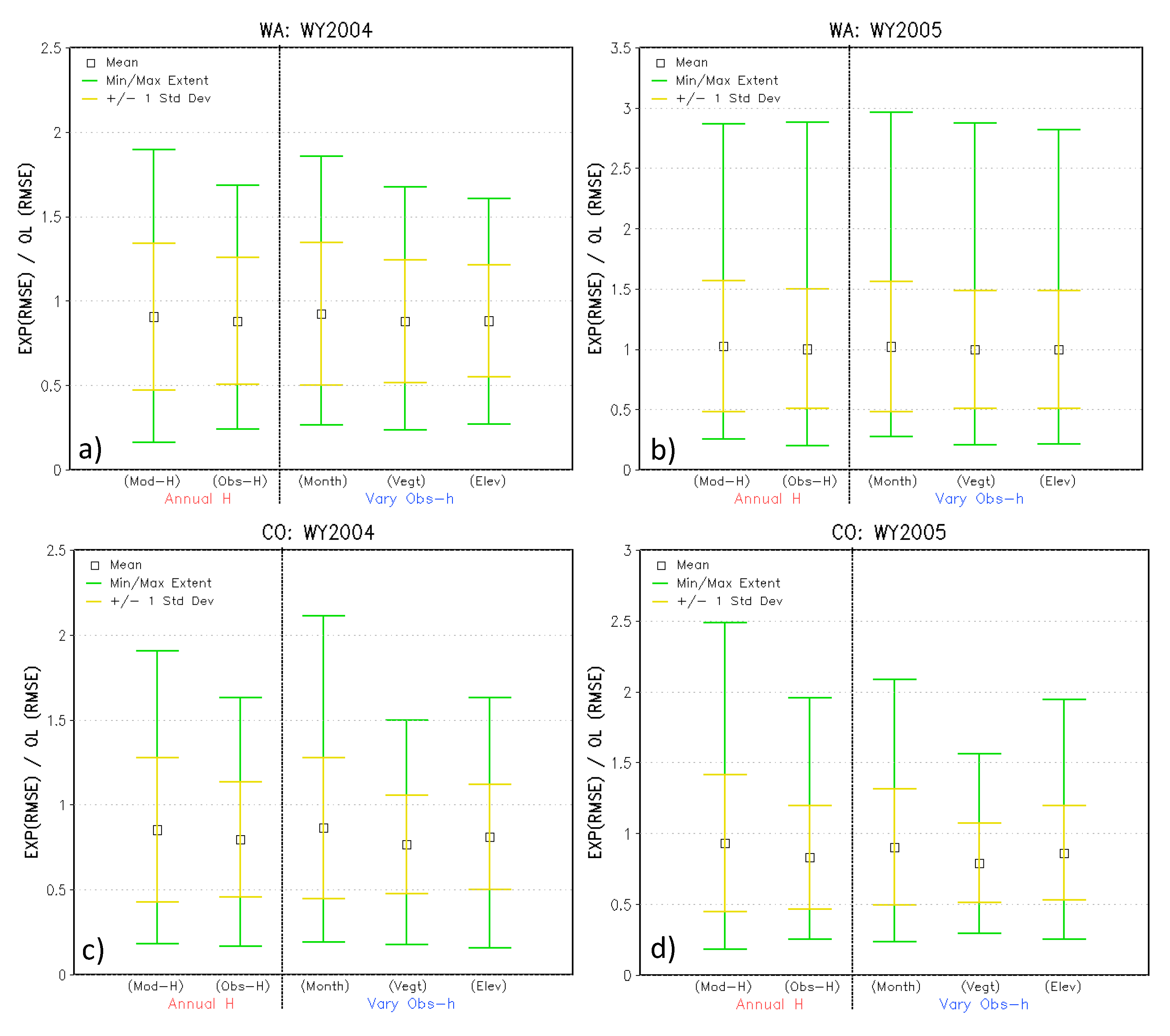
To show how the RMSE values of each DA experiment relate to the open-loop run, Figure 7 shows each experiment’s SWE-based RMSE values normalized with respect to those of the open-loop based on [51]. A normalized RMSE value less than one indicates the experiment may perform better than its control run, which is the open-loop in this case [51]. All experiments perform better than the open-loop runs, except for WA’s WY2005, which was a major drought year and difficult to capture with the ensembles and observations. Also, the ±1 standard deviation values (inner yellow error bars) in Figure 7 show smaller ranges for many of the obs-h experiments, especially the vegetation obs-h case for CO.
To see how this performance translates into EnKF metrics, the normalized innovation means and standard deviations for each experiment and water year are provided in Table 3. The means tend slightly closer to 0 for the obs-h than the model-h based experiments, indicating differences between the individual MODIS SCF values and model predicted SCF values were overall smaller. This may suggest that the obs-h curves predicted SCF values that were in slightly better agreement with the MODIS observations. The exception again was WY2005 for WA where there were greater differences, indicated by much higher negative mean values. This may relate to the shape of the curves and thus predicting higher SCF forecast values than the MODIS estimates. For the normalized innovation standard deviations, the values increase to near 1 with almost all the obs-h experiments, which may indicate that the model errors and observational errors may be more consistent in the filter (e.g., [52]) than those associated with the model-h EnKF experiments. This could possibly indicate better agreement in MODIS SCF values with the model predicted SCF produced by the obs-h curves.
6. Discussion
In this study, we have explored how different observation-based snow depletion curve (SDC) characteristics can be derived and used as observation-based observation operators in EnKF assimilation updates when assimilating MODIS, or other satellite-based, snow cover fraction estimates. Different SDC logarithmic functions, representing different physiographic and temporal conditions, were also explored as observation-based observation operators in a full suite of EnKF experiments. Using logarithmic functions with a y-axis intercept value, not set to 0, means that MODIS SCF values may not be assimilated below that value (e.g., 40% SCF). In a way, this acts as a cutoff for lower MODIS SCF values (e.g., less than 30%), which could contain contaminated SCF values, due to unresolved patchiness in a pixel and NDSI algorithm pixel discrimination issues [53]. Also, the fact that many of the logarithmic curves never fully reach 100% SCF could allow MODIS SCF pixels that are near 100% to have an impact on the snow analysis, when the model SCF forecasts are much lower than 100%. This situation can work well when the LSM consistently underestimates SWE, relative to the in situ SWE observations. Therefore, for LSMs with a low SWE bias or precipitation input bias (e.g., an undercatch issue), this SDC approach can partly compensate for the low bias, especially when assimilating snow cover in higher mountain catchments locations. However, if an LSM or snow model has a high SWE bias compared to the observations, then this observed type SDC could contribute to overestimating and adding too much snow to the model.
In other snow cover data assimilation studies, most curves are designed to reach 100% SCF, even for coarser grid scale experiments [13]. If model SWE forecast conditions remain high enough that the predicted SCF ensemble forecasts remain at 100%, with little ensemble spread in SCF, then there can be very little to no impact on the SWE analysis if the observed SCF is much less than 100%, e.g., partial coverage for the gridcell [14]. Another minor downside to having an SDC-type observation operator reach 100% snow cover, like the case for many LSM curves, the EnKF-based model SCF forecast ensemble can become underestimated, if perturbations force the members to fall below 100%, even if both the MODIS and model predicted SCF were originally at 100%. This can also occur when perturbing the MODIS SCF observations. When the observed SCF is at 100%, this can also reduce that value when perturbed, leading to underestimated SWE analysis [14]. Rules can be applied in the EnKF method as to how the ensemble members, e.g., within the observation-perturbed ensemble, get distributed or updated near the 100% SCF point. This could include a set of rules for reducing the SWE analysis by a certain fraction when there is a partial amount of observed SCF or by modifying the observation error covariance, σtotal, that controls the ensemble or uncertainty spread [based on 14]. One slight advantage to the SNOTEL-MODIS observation-based observation operators, obs-h, is that they reflect an average SCF percentage of what the satellite detects for a given range of conditions. Thus, if the predicted SCF is 80% and is the upper threshold in the SDC function, then 20% of the area could be considered exposed vegetation cover or average SCF conditions, for say, lower elevation regions.
Based on the filter statistics shown in Table 2 and Table 3, there still remains some large differences between the magnitudes of the model predicted SCF and the MODIS SCF observations. One approach to address these innovation biases would be to scale the MODIS SCF values to reflect higher ones, bringing them into closer agreement with the predicted SCF values [54]. Another option would be to place additional constraints on the observation operators or SCF observations themselves, or to further tune the observations or the curves towards the other, so that the filter statistics reflect less bias between observations and the model. In this study, by deriving the observation-based observation operators with the MODIS SCF observations, it helps to bring the predicted SCF values closer in agreement to the observations. With almost all data assimilation approaches, tuning may be the unavoidable course to be taken, so the final analysis may reflect the best that both the model and observations have to offer.
7. Conclusions
In this study, we presented a new approach to estimating snow depletion curves and their application for assimilating snow cover fraction observations, using an EnKF approach and a land surface model with a multi-layer snow physics scheme. We use observed SWE and snow cover fraction estimates to derive new SDCs, using a larger array of observations than previous studies, spanning two different mountainous regions in the U.S., in Washington and Colorado. We refer to these new SDC observation operators as “observation-based” and benchmarked their skill against the default, model-based SDC function. The SDC observation-based observation operators showed improvement over the default model-based SCF forecasts and snow state analysis. A secondary goal of this study was to apply this SDC-type approach to see how accounting for varying vegetation, elevation, and temporal conditions may better capture heterogeneous features related to the snowpack and snow cover patterns when assimilating snow cover observations. Vegetation-based curves showed improvement over the lumped annual observation-based SDC, especially for Colorado. Finally, the new SDC-based observation operators are used to derive the observational errors, which were used in the EnKF method’s snow cover observation perturbations. Accounting for different errors related to the varying conditions provides different weighting of the snow cover observations against that of the model in the EnKF innovation and update steps.
These results along with other previous SCA DA studies do show promise in that there are positive impacts without much tuning, but additional testing with the observation operators, model, and observations is still needed [10,18]. In future work, more a priori information about the MODIS SCF predictions could be included to deriving and tuning functions, like the ones developed here for this DA application. For example, determining error information with regard to MODIS SCF 100% estimates in connection with the meteorological forcing fields, e.g., ability to estimate snowfall for same observed 100% SCF events or the role that temperature can play in MODIS SCA errors [55]. Also, more adaptive type SDC schemes, which could be more representative at a point, could be developed that adjust relative to changing conditions. Different approaches could be applied to optimize these observational based SDCs and improve the overall performance of the EnKF system.
Supplementary Materials
The following are available online at https://www.mdpi.com/2076-3263/8/12/484/s1, Figure S1: Presenting the binned scatterplots for the two mountain regions. Figure S2: Showing the robustness of the scatterbin histogram approach for deriving the SDCs. Figure S3: Monthly SDC relationships derived from binned scatterplot approach for the Washington state domain. Figure S4: Similar to Figure S3, but for Colorado state domain. Figure S5: SDC relationships derived for two different elevation bands for Washington domain. Figure S6: Similar to Figure S5, but for the Colorado domain. Figure S7: SDC relationships derived for different vegetation types from binned scatterplot approach for Washington. Figure S8: Similar to Figure S7, but for Colorado. Figure S9: Independent check on the snow water equivalent bins for different dominant vegetation types and in relation to elevation, for Washington domain. Figure S10: Similar to Figure S9, but for Colorado. Figure S11: Timeseries comparison of the experiments’ spatially averaged predicted SCF (in %) for the different observation operators and SCF observations, presented for the melt season. Figure S12: Individual SNOTEL site comparisons between different SDC-type observation operators.
Author Contributions
Much of the work, including methodology, code development, validation and analysis, was performed by K.R.A., and overall supervision and funding acquisition was provided by P.R.H. The original draft preparation and writing was done by K.R.A., and review and editing was done by P.R.H.
Funding
This research was originally funded by grants given by the U.S. National Oceanic and Atmospheric Administration and the National Aeronautics and Space Administration.
Acknowledgments
We want to acknowledge the original support and computing resources provided by The Center for Ocean-Land-Atmosphere Studies (COLA) at George Mason University in Fairfax, Virginia, U.S.A.
Conflicts of Interest
The authors declare no conflict of interest.
References
- Qu, X.; Hall, A. Assessing Snow Albedo Feedback in Simulated Climate Change. J. Clim. 2006, 19, 2617–2630. [Google Scholar] [CrossRef] [Green Version]
- Fassnacht, S.R.; Sexstone, G.A.; Kashipazha, A.H.; Lopez-Moreno, J.I.; Jasinski, M.F.; Kampf, S.K.; Von Thaden, B.C. Deriving snow-cover depletion curves for different spatial scales from remote sensing and snow telemetry data. Hydrol. Process. 2016, 30, 1708–1717. [Google Scholar] [CrossRef]
- Driscoll, J.M.; Hay, L.E.; Bock, A. Spatiotemporal Variability of Snow Depletion Curves Derived from SNODAS for the Conterminous United States, 2004–2013. J. Am. Water Resour. Assoc. 2017, 53, 655–666. [Google Scholar] [CrossRef]
- Liston, G.E. Representing subgrid snow cover heterogeneities in regional and global models. J. Clim. 2004, 17, 1381–1397. [Google Scholar] [CrossRef]
- Anderson, E.A. National Weather Service River Forecast System: Snow Accumulation and Ablation Model; NWS HYDRO-17; NOAA Technical Memorandum; NOAA: Silver Spring, MD, USA, 1973.
- Donald, J.R.; Soulis, E.D.; Kouwen, N.; Pietroniro, A. A land cover-based snow cover representation for distributed hydrologic-models. Water Resour. Res. 1995, 31, 995–1009. [Google Scholar] [CrossRef]
- Kolberg, S.A.; Gottschalk, L. Updating of snow depletion curve with remote sensing data. Hydrol. Process. 2006, 20, 2363–2380. [Google Scholar] [CrossRef]
- Shamir, E.; Georgakakos, K.P. Estimating snow depletion curves for American River basins using distributed snow modeling. J. Hydrol. 2007, 334, 162–173. [Google Scholar] [CrossRef]
- DeBeer, C.M.; Pomeroy, J.W. Influence of snowpack and melt energy heterogeneity on snow cover depletion and snowmelt runoff simulation in a cold mountain environment. J. Hydrol. 2017, 553, 199–213. [Google Scholar] [CrossRef]
- Andreadis, K.M.; Lettenmaier, D.P. Assimilating remotely sensed snow observations into a macroscale hydrology model. Adv. Water Resour. 2006, 29, 872–886. [Google Scholar] [CrossRef]
- Kolberg, S.; Rue, H.; Gottschalk, L. A Bayesian spatial assimilation scheme for snow coverage observations in a gridded snow model. Hydrol. Earth Syst. Sci. 2006, 10, 369–381. [Google Scholar] [CrossRef] [Green Version]
- Zaitchik, B.; Rodell, M. Forward-looking assimilation of MODIS-derived snow-covered area into a land surface model. J. Hydrometeorol. 2009, 10, 130–148. [Google Scholar] [CrossRef]
- Su, H.; Yang, Z.-L.; Niu, G.-Y.; Dickinson, R.E. Enhancing the estimation of continental-scale snow water equivalent by assimilation MODIS snow cover with the ensemble Kalman filter. J. Geophys. Res. 2008, 113, D08120. [Google Scholar] [CrossRef]
- De Lannoy, G.J.M.; Reichle, R.H.; Arsenault, K.R.; Houser, P.R.; Kumar, S.; Verhoest, N.E.C.; Pauwels, V.R.N. Multiscale assimilation of Advanced Microwave Scanning Radiometer-EOS snow water equivalent and Moderate Resolution Imaging Spectroradiometer snow cover fraction observations in northern Colorado. Water Resour. Res. 2012, 48, W01522. [Google Scholar] [CrossRef]
- Arsenault, K.R.; Houser, P.R.; De Lannoy, G.J.M.; Dirmeyer, P.A. Impacts of snow cover fraction data assimilation on modeled energy and moisture budgets. J. Geophys. Res. Atmos. 2013, 118, 7489–7504. [Google Scholar] [CrossRef] [Green Version]
- Zhang, Y.-F.; Hoar, T.J.; Yang, Z.-L.; Anderson, J.L.; Toure, A.M.; Rodell, M. Assimilation of MODIS snow cover through the Data Assimilation Research Testbed and the Community Land Model version 4. J. Geophys. Res. Atmos. 2014, 119, 7091–7103. [Google Scholar] [CrossRef] [Green Version]
- Xu, J.; Zhang, F.; Shu, H.; Zhong, K. Improvement of the Snow Depth in the Common Land Model by Coupling a Two-Dimensional Deterministic Ensemble Model with a Variational Hybrid Snow Cover Fraction Data Assimilation Scheme and a New Observation Operator. J. Hydrometeorol. 2017, 18, 119–138. [Google Scholar] [CrossRef]
- Clark, M.P.; Slater, A.G.; Barrett, A.P.; Hay, L.E.; McCabe, G.J.; Rajagopalan, B.; Leavesley, G.H. Assimilation of snow-covered area information into hydrologic and land-surface models. Adv. Water Resour. 2006, 29, 1209–1221. [Google Scholar] [CrossRef]
- Thirel, G.; Salamon, P.; Burek, P.; Kalas, M. Assimilation of MODIS snow cover area data in a distributed hydrological model using the particle filter. Remote Sens. 2013, 5, 5825–5850. [Google Scholar] [CrossRef]
- Niu, G.-Y.; Yang, Z.-L. An observation-based formulation of snow cover fraction and its evaluation over large North American river basins. J. Geophys. Res. 2007, 112, D21101. [Google Scholar] [CrossRef]
- Salomonson, V.V.; Appel, I. Estimating fractional snow cover from MODIS using the normalized difference snow index. Remote Sens. Environ. 2004, 89, 351–360. [Google Scholar] [CrossRef]
- Hall, D.K.; Riggs, G.A. Accuracy Assessment of the MODIS snow products. Hydrol. Process. 2007, 21, 1534–1547. [Google Scholar] [CrossRef]
- Salomonson, V.V.; Appel, I. Development of the Aqua MODIS NDSI fractional snow cover algorithm and validation results. IEEE Trans. Geosci. Remote Sens. 2006, 44, 1747–1756. [Google Scholar] [CrossRef]
- Hall, D.K.; Riggs, G.A. MODIS/Terra Snow Cover Daily L3 Global 500 m Grid, Version 5; NASA National Snow and ICE Data Center Distributed Active Archive Center: Boulder, CO, USA, 2011. [CrossRef]
- Parajka, J.; Holko, L.; Kostka, Z.; Bloschl, G. MODIS snow cover mapping accuracy in a small mountain catchment—Comparison between open and forest sites. Hydrol. Earth Syst. Sci. 2012, 16, 2365–2377. [Google Scholar] [CrossRef]
- Dwyer, J.; Schmidt, G. The MODIS Reprojection Tool. In Earth Science Satellite Remote Sensing; Qu, J.J., Gao, W., Kafatos, M., Murphy, R.E., Salomonson, V.V., Eds.; Springer: Berlin/Heidelberg, Germany, 2006. [Google Scholar]
- National Climatic Data Center. Data Documentation for Dataset 6430 (DSI-6430), USDA/NRCS SNOTEL—Daily Data; Text Reports; NCDC: Asheville, NC, USA, 2002.
- Pan, M.; Sheffield, J.; Wood, E.F.; Mitchell, K.E.; Houser, P.R.; Schaake, J.C.; Robock, A.; Lohmann, D.; Cosgrove, B.; Duan, Q.; et al. Snow process modeling in the North American Land Data Assimilation System (NLDAS): 2. Evaluation of model simulated snow water equivalent. J. Geophys. Res. 2003, 108. [Google Scholar] [CrossRef] [Green Version]
- Serreze, M.C.; Clark, M.P.; Armstrong, R.L.; McGinnis, D.A.; Pulwarty, R.S. Characteristics of the western United States snowpack from snowpack telemetry (SNOTEL) data. Water Resour. Res. 1999, 35, 2145–2160. [Google Scholar] [CrossRef] [Green Version]
- Bonan, G.B.; Oleson, K.W.; Vertenstein, M.; Levis, S.; Zeng, X.; Dai, Y.; Dickinson, R.E.; Yang, Z.-L. The land surface climatology of the Community Land Model coupled to the NCAR Community Climate Model. J. Clim. 2002, 15, 3123–3149. [Google Scholar] [CrossRef]
- Dai, Y.; Zeng, X.; Dickinson, R.E.; Baker, I.; Bonan, G.B.; Bosilovich, M.G.; Denning, A.S.; Dirmeyer, P.A.; Houser, P.R.; Niu, G.; et al. The Common Land Model. Bull. Am. Meteorol. Soc. 2003, 84, 1013–1023. [Google Scholar] [CrossRef]
- Oleson, K.W.; Dai, Y.; Bonan, G.; Bosilovich, M.; Dickinson, R.; Dirmeyer, P.; Hoffman, F.; Houser, P.; Levis, S.; Niu, G.-Y.; et al. Technical Description of the Community Land Model (CLM); NCAR Technical Note; NCAR/TN-461+STR; Center for Atmospheric Research: Boulder, CO, USA, 2004. [Google Scholar]
- Kumar, S.V.; Peters-Lidard, C.D.; Tian, Y.; Houser, P.R.; Geiger, J.; Olden, S.; Lighty, L.; Eastman, J.L.; Doty, B.; Dirmeyer, P.; et al. Land Information System—An Interoperable Framework for High Resolution Land Surface Modeling. Environ. Model. Softw. 2006, 21, 1402–1415. [Google Scholar] [CrossRef]
- Anderson, E.A. A Point Energy and Mass Balance Model of a Snow Cover; NOAA Technical Report NWS 19; Office of Hydrology, National Weather Service: Silver Spring, MD, USA, 1976.
- Jordan, R. A One-Dimensional Temperature Model for a Snow Cover: Technical Documentation for SNTHERM.89; Special Report 91-16; U.S. Army Cold Regions Research and Engineering Laboratory: Hanover, NH, USA, 1991. [Google Scholar]
- Dai, Y.; Zeng, Q. A land surface model (IAP94) for climate studies. Part I: Formulation and validation in off-line experiments. Adv. Atmos. Sci. 1997, 14, 433–460. [Google Scholar]
- Feng, X.; Sahoo, A.; Arsenault, K.; Houser, P.; Luo, Y.; Troy, T.J. The Impact of Snow Model Complexity at Three CLPX Sites. J. Hydrometeorol. 2008, 9, 1464–1481. [Google Scholar] [CrossRef]
- Rutter, N.; Essery, R.; Pomeroy, J.; Altimir, N.; Andreadis, K.; Baker, I.; Barr, A.; Bartlett, P.; Boone, A.; Deng, H.; et al. Evaluation of forest snow process models (SnowMIP2). J. Geophys. Res. 2009, 114, D06111. [Google Scholar] [CrossRef]
- Wang, A.; Zeng, X. Improving the treatment of vertical snow burial fraction over short vegetation in the NCAR CLM3. Adv. Atmos. Sci. 2009, 26, 877–886. [Google Scholar] [CrossRef]
- Cosgrove, B.A.; Lohmann, D.; Mitchell, K.E.; Houser, P.R.; Wood, E.F.; Schaake, J.C.; Robock, A.; Marshall, C.; Sheffield, J.; Duan, Q.; et al. Real-time and retrospective forcing in the North American Land Data Assimilation System (NLDAS) project. J. Geophys. Res. 2003, 108, 8842. [Google Scholar] [CrossRef]
- Friedl, M.A.; McIver, D.K.; Hodges, J.C.F.; Zhang, X.Y.; Muchoney, D.; Strahler, A.H.; Woodcock, C.E.; Gopal, S.; Schneider, A.; Cooper, A.; et al. Global land cover classification at 1km spatial resolution using a classification tree approach. Remote Sens. Environ. 2002, 83, 287–302. [Google Scholar] [CrossRef]
- Reichle, R.H.; McLaughlin, D.B.; Entekhabi, D. Hydrologic data assimilation with the Ensemble Kalman filter. Mon. Weather Rev. 2002, 130, 103–114. [Google Scholar] [CrossRef]
- Reichle, R.H.; Bosilovich, M.G.; Crow, W.T.; Koster, R.D.; Kumar, S.V.; Mahanama, S.P.P.; Zaitchik, B.F. Recent Advances in Land Data Assimilation at the NASA Global Modeling and Assimilation Office. In Data Assimilation for Atmospheric, Oceanic and Hydrologic Applications; Park, S.K., Xu, L., Eds.; Springer: New York, NY, USA, 2009; pp. 407–428. [Google Scholar] [CrossRef]
- Kumar, S.V.; Reichle, R.H.; Peters-Lidard, C.D.; Koster, R.D.; Zhan, X.; Crow, W.T.; Eylander, J.B.; Houser, P.R. A land surface data assimilation framework using the land information system: Description and applications. Adv. Water Resour. 2008, 31, 1419–1432. [Google Scholar] [CrossRef]
- Bowling, L.C.; Pomeroy, J.W.; Lettenmaier, D.P. Parameterization of blowing-snow sublimation in a macroscale hydrology model. J. Hydrometeorol. 2004, 5, 745–762. [Google Scholar] [CrossRef]
- Jacko, J.A.; Stephanidis, C. (Eds.) Human-Computer Interaction: Theory and Practice; Lawrence Erlbaum and Associates: Mahwah, NJ, USA, 2003. [Google Scholar]
- Seo, H.; Miller, A.J.; Roads, J.O. The Scripps Coupled Ocean-Atmosphere Regional (SCOAR) Model, with Applications in the Eastern Pacific Sector. J. Clim. 2007, 20, 381–402. [Google Scholar] [CrossRef]
- Jost, G.; Weiler, M.; Gluns, D.R.; Alila, Y. The influence of forest and topography on snow accumulation and melt at the watershed-scale. J. Hydrol. 2007, 347, 101–115. [Google Scholar] [CrossRef]
- Anderton, S.P.; White, S.M.; Alvera, B. Evaluation of spatial variability in snow water equivalent for a high mountain catchment. Hydrol. Process. 2004, 18, 435–453. [Google Scholar] [CrossRef]
- Molotch, N.P.; Margulis, S.A. Estimating the distribution of snow water equivalent using remotely sensed snow cover data and a spatially distributed snowmelt model: A multi-resolution, multi-sensor comparison. Adv. Water Res. 2008, 31, 1503–1514. [Google Scholar] [CrossRef]
- Crow, W.T.; Ryu, D. A new data assimilation approach for improving runoff prediction using remotely-sensed soil moisture retrievals. Hydrol. Earth Syst. Sci. 2009, 13, 1–16. [Google Scholar] [CrossRef] [Green Version]
- Whitaker, J.S.; Hamill, T.M.; Wei, X.; Song, Y.; Toth, Z. Ensemble data assimilation with the NCEP Global Forecast System. Mon. Weather Rev. 2008, 136. [Google Scholar] [CrossRef]
- Déry, S.J.; Salomonson, V.V.; Stieglitz, M.; Hall, D.K.; Appel, I. An approach to using snow areal depletion curves inferred from MODIS and its application to land surface modelling in Alaska. Hydrol. Process. 2005, 19, 2755–2774. [Google Scholar] [CrossRef]
- Xu, L.; Dirmeyer, P. Snow-atmosphere coupling strength. Part I: Effect of model biases. J. Hydrometeorol. 2013, 14, 389–403. [Google Scholar] [CrossRef]
- Dong, J.; Peters-Lidard, C. On the relationship between temperature and MODIS snow cover retrieval errors in the Western U.S. IEEE J. Sel. Top. Appl. Earth Obs. Remote Sens. 2010, 3, 132–140. [Google Scholar] [CrossRef]
Figure 1.
Elevation maps of Washington and Colorado domains, from the U.S. Geological Survey (USGS) National Elevation Dataset (NED) dataset. All SNOwpack TELemetry (SNOTEL) site (black triangles) are used in generating the observation-based snow depletion curves (SDCs), and a reduced amount of site locations are used only in the model experiments and validation (grey open circles).

Figure 2.
The binned scatterplot bin averages for Washington (WA) (large red squares) and Colarado (CO) (larger green triangles) imposed over all scatter plot points that are used in generating the bins. Logarithmic functions are fitted here to the binned snow cover fraction (SCF) averages with the red (green) line corresponding to the equation and R2 value in the lower right-hand side red (green) box for WA (CO).

Figure 3.
Comparison of the different SDC-observation operators (h), including the Community Land Model-based SDCs (CLM2 and CLM4-Niu and Yang (2007; NY07), and the observation-based observation operators (obs-h) for WA (maroon dashes) and CO (orange dashes). The 40 mm snow water equivalent (SWE) values are used in the CLM curves (model-h) to derive SCF estimates for this comparison. For the CLM2 curve, three different snow densities are used to show snow-depth to SWE (100, 250, 400 kg m−3) ranges in SCF estimates, and the NY07 curve for just the 250 kg m−3 snow density value is used (navy blue diamonds).

Figure 4.
A bar plot of the varying observation standard error values, σtotal, (in % of SCF) for each given set of derived observation-based observation operators, obs-h, including annual-based, monthly, vegetation type and elevation band. Blue (red) bars indicate observation errors associated with CO (WA).

Figure 5.
Spatially averaged SWE comparison is made between SNOTEL observations (open circles), the OL run (grey line), model-h EnKF experiment (red line), and obs-h EnKF (green line) experiments for both (a) WA and (b) CO regions. Values given within the parentheses indicate the σtotal values for the experiment.

Figure 6.
Spatially averaged RMSE SWE values (in mm) for both (a) WA and (b) CO for the OL run (grey line), model-h EnKF (red line) and obs-h EnKF (green line) experiments.
Figure 6.
Spatially averaged RMSE SWE values (in mm) for both (a) WA and (b) CO for the OL run (grey line), model-h EnKF (red line) and obs-h EnKF (green line) experiments.

Figure 7.
Comparison of each experiment’s SWE RMSE values normalized by the open-loop (OL) RMSE values for the five experiments: Model-h EnKF run, and the annual, monthly, vegetation, and elevation varying obs-h EnKF experiments for WA (a,b) and CO (c,d) for WY2004 (left) and WY2005 (right). Black open squares indicate the statistical mean, yellow error bar lines indicate ±1 stdev unit from mean, and green error bar lines indicate the maximum and minimum extents of the normalized statistic. Values below 1 suggest improvement over the OL run.


Table 1.
A summary table of the different baseline and data assimilation-based experiments and the naming convention used for each experiment. Same experiments were conducted for both WA and CO domains over the water years, 2004 and 2005.
Table 1.
A summary table of the different baseline and data assimilation-based experiments and the naming convention used for each experiment. Same experiments were conducted for both WA and CO domains over the water years, 2004 and 2005.
| Experiment Name | Description |
|---|---|
| Open-loop (OL) | The baseline ensemble model experiment with no snow cover assimilation performed. |
| EnKF: Model-h | Snow cover assimilation using EnKF and the default model-based SDC as the observation operator. |
| EnKF: Annual obs-h | Snow cover assimilation using EnKF and the annual observation-based SDC as the observation operator. |
| EnKF: Month-based obs-h | Snow cover assimilation using EnKF and the monthly-varying, observation-based SDCs as the observation operator. |
| EnKF: Vegetation-based obs-h | Snow cover assimilation using EnKF and the vegetation-type, observation-based SDCs as the observation operator. |
| EnKF: Elevation band-based obs-h | Snow cover assimilation using EnKF and the elevation-band, observation-based SDCs as the observation operator. |
Table 2.
Comparison of summary SWE statistics for the period, October-June, between observation operator experiments. Bold numbers indicate experiments with reduced RMSE values relative to the open-loop and model-h EnKF experiments. SD refers to standard deviation.
Table 2.
Comparison of summary SWE statistics for the period, October-June, between observation operator experiments. Bold numbers indicate experiments with reduced RMSE values relative to the open-loop and model-h EnKF experiments. SD refers to standard deviation.
| Observation Operator Comparison Statistics | ||||||||
|---|---|---|---|---|---|---|---|---|
| Average | SD | RMSE | Correl | Average | SD | RMSE | Correl | |
| (mm) | (mm) | (mm) | (-) | (mm) | (mm) | (mm) | (-) | |
| WA (40 Sites) | 2004 | 2005 | ||||||
| Observations | 221.85 | 216.19 | - | - | 61.19 | 66.56 | - | - |
| Open-loop | 247.01 | 188.17 | 168.22 | 0.79 | 64.30 | 61.14 | 65.09 | 0.74 |
| EnKF: Model-h | 183.54 | 184.21 | 138.54 | 0.87 | 34.62 | 40.38 | 60.29 | 0.75 |
| EnKF: Annual obs-h | 194.09 | 191.40 | 140.13 | 0.87 | 40.11 | 45.38 | 57.46 | 0.75 |
| EnKF: Month obs-h | 191.09 | 191.31 | 145.33 | 0.85 | 37.27 | 42.89 | 58.29 | 0.74 |
| EnKF: Veg. obs-h | 195.79 | 192.18 | 140.28 | 0.87 | 40.60 | 45.77 | 57.31 | 0.75 |
| EnKF: Elev. obs-h | 199.91 | 193.46 | 142.41 | 0.87 | 40.80 | 46.07 | 57.83 | 0.75 |
| CO (78 Sites) | 2004 | 2005 | ||||||
| Observations | 132.74 | 127.26 | - | - | 187.20 | 168.07 | - | - |
| Open-loop | 143.75 | 115.63 | 107.00 | 0.72 | 180.14 | 132.52 | 127.97 | 0.79 |
| EnKF: Model-h | 94.01 | 92.34 | 81.57 | 0.89 | 119.57 | 109.58 | 116.57 | 0.89 |
| EnKF: Annual obs-h | 108.00 | 105.82 | 79.24 | 0.88 | 139.72 | 127.99 | 103.69 | 0.91 |
| EnKF: Month obs-h | 111.15 | 109.82 | 86.21 | 0.86 | 145.82 | 134.43 | 109.96 | 0.89 |
| EnKF: Veg. obs-h | 114.26 | 111.18 | 76.91 | 0.88 | 147.93 | 134.33 | 99.51 | 0.91 |
| EnKF: Elev. obs-h | 112.60 | 109.71 | 81.74 | 0.87 | 144.87 | 132.64 | 108.19 | 0.90 |
Table 3.
Table of normalized innovation values, including the mean and standard deviation (SD) for the different observation operator, h, experiments.
Table 3.
Table of normalized innovation values, including the mean and standard deviation (SD) for the different observation operator, h, experiments.
| Normalized Innovation Analysis | ||||||||
|---|---|---|---|---|---|---|---|---|
| WA | CO | |||||||
| 2004 | 2005 | 2004 | 2005 | |||||
| Experiment | Mean | SD | Mean | SD | Mean | SD | Mean | SD |
| CLM2 mod-h | −0.43 | 0.89 | −0.39 | 0.81 | −0.43 | 0.92 | −0.37 | 0.87 |
| Annual obs-h | −0.41 | 0.99 | −0.57 | 0.95 | −0.42 | 0.98 | −0.34 | 0.94 |
| Monthly obs-h | −0.41 | 0.97 | −0.59 | 0.98 | −0.38 | 1.02 | −0.31 | 0.93 |
| Veg. obs-h | −0.41 | 1.02 | −0.58 | 0.95 | −0.39 | 1.01 | −0.30 | 0.97 |
| Elev. obs-h | −0.41 | 1.00 | −0.57 | 0.95 | −0.41 | 1.02 | −0.32 | 0.99 |
© 2018 by the authors. Licensee MDPI, Basel, Switzerland. This article is an open access article distributed under the terms and conditions of the Creative Commons Attribution (CC BY) license (http://creativecommons.org/licenses/by/4.0/).
Share and Cite
MDPI and ACS Style
Arsenault, K.R.; Houser, P.R. Generating Observation-Based Snow Depletion Curves for Use in Snow Cover Data Assimilation. Geosciences 2018, 8, 484. https://doi.org/10.3390/geosciences8120484
AMA Style
Arsenault KR, Houser PR. Generating Observation-Based Snow Depletion Curves for Use in Snow Cover Data Assimilation. Geosciences. 2018; 8(12):484. https://doi.org/10.3390/geosciences8120484
Chicago/Turabian StyleArsenault, Kristi R., and Paul R. Houser. 2018. "Generating Observation-Based Snow Depletion Curves for Use in Snow Cover Data Assimilation" Geosciences 8, no. 12: 484. https://doi.org/10.3390/geosciences8120484
Note that from the first issue of 2016, this journal uses article numbers instead of page numbers. See further details here.