Geomorphology and Late Pleistocene–Holocene Sedimentary Processes of the Eastern Gulf of Finland

Abstract
:1. Introduction
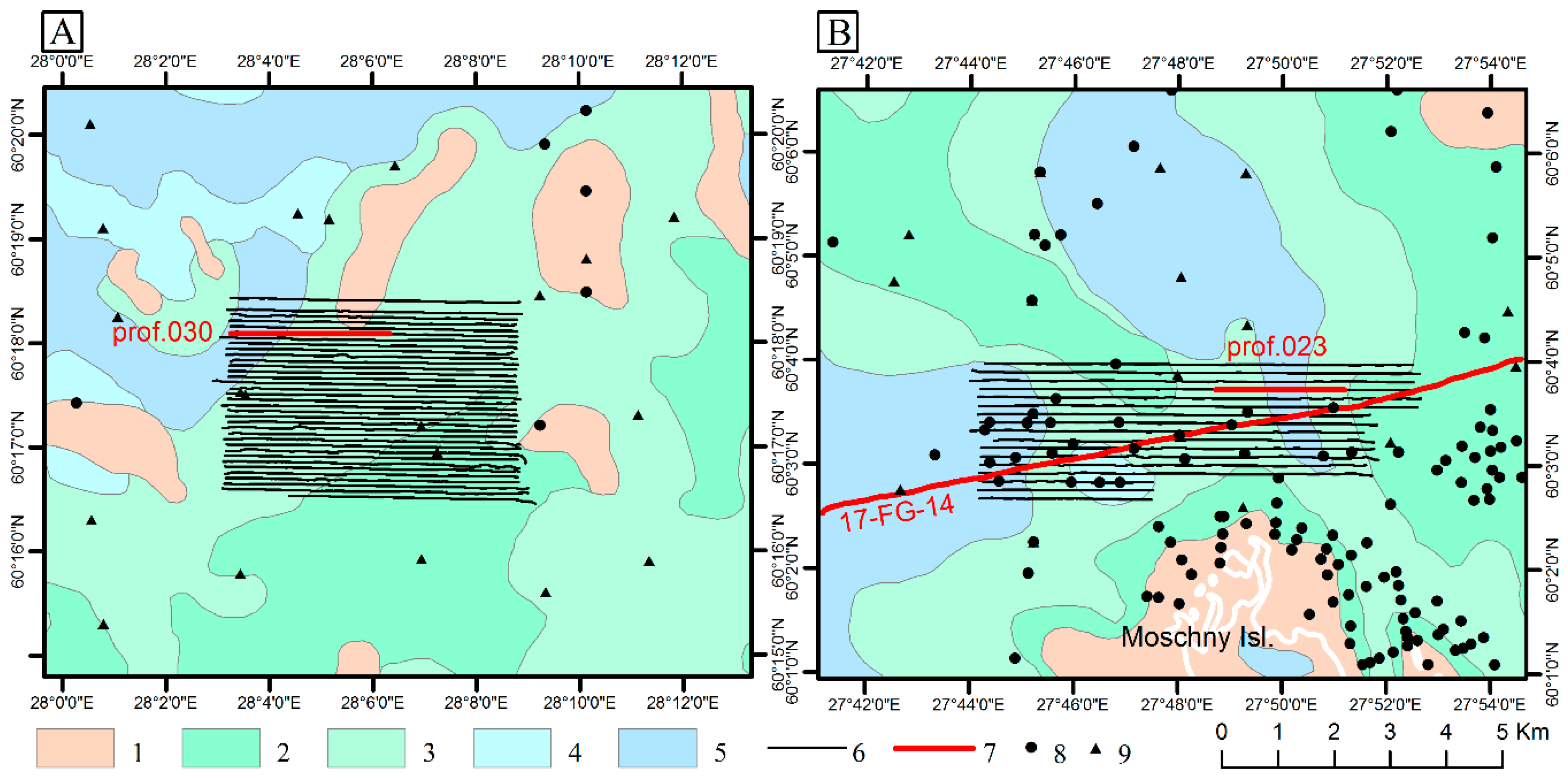
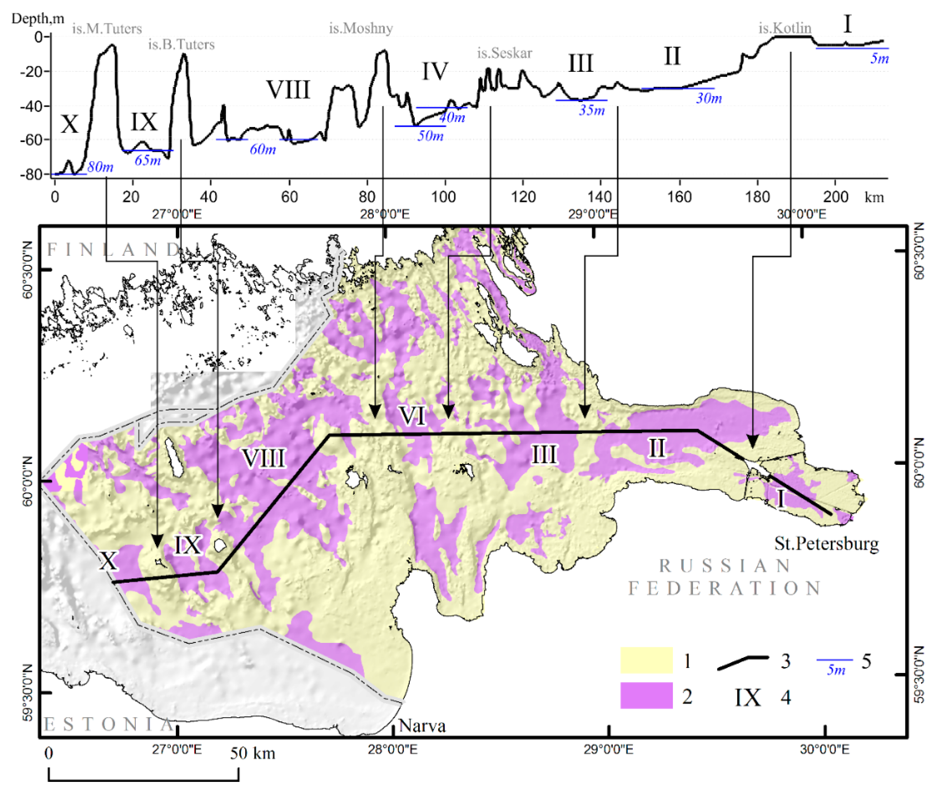
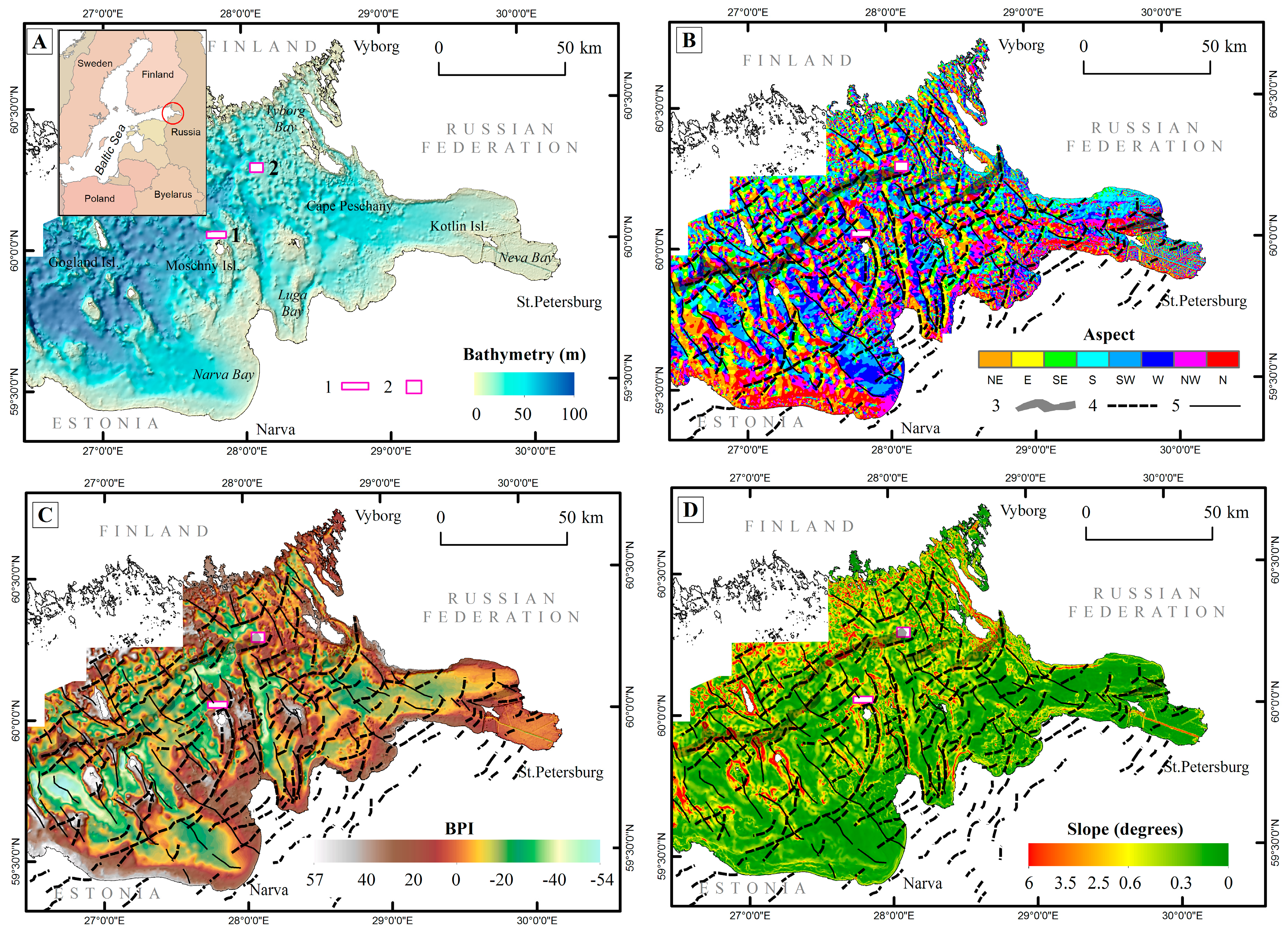
Study Area
2. Material and Methods
2.1. Broad-Scale Data Analysis
2.2. Multibeam Echosounding and Acoustic-Seismic Profiling Equipment
2.3. Calibration
2.4. Multibeam Bathymetry Data Processing
2.4.1. Stage 1. Initial Data Processing Using the Default Software Package, PDS2000
2.4.2. Stage 2. Data Import into ArcGIS and Generation of the Digital Bathymetric Model (DBM)
2.4.3. Stage 3. Reduction of Bathymetric Data Artefacts with the Use of the ArcGIS Software
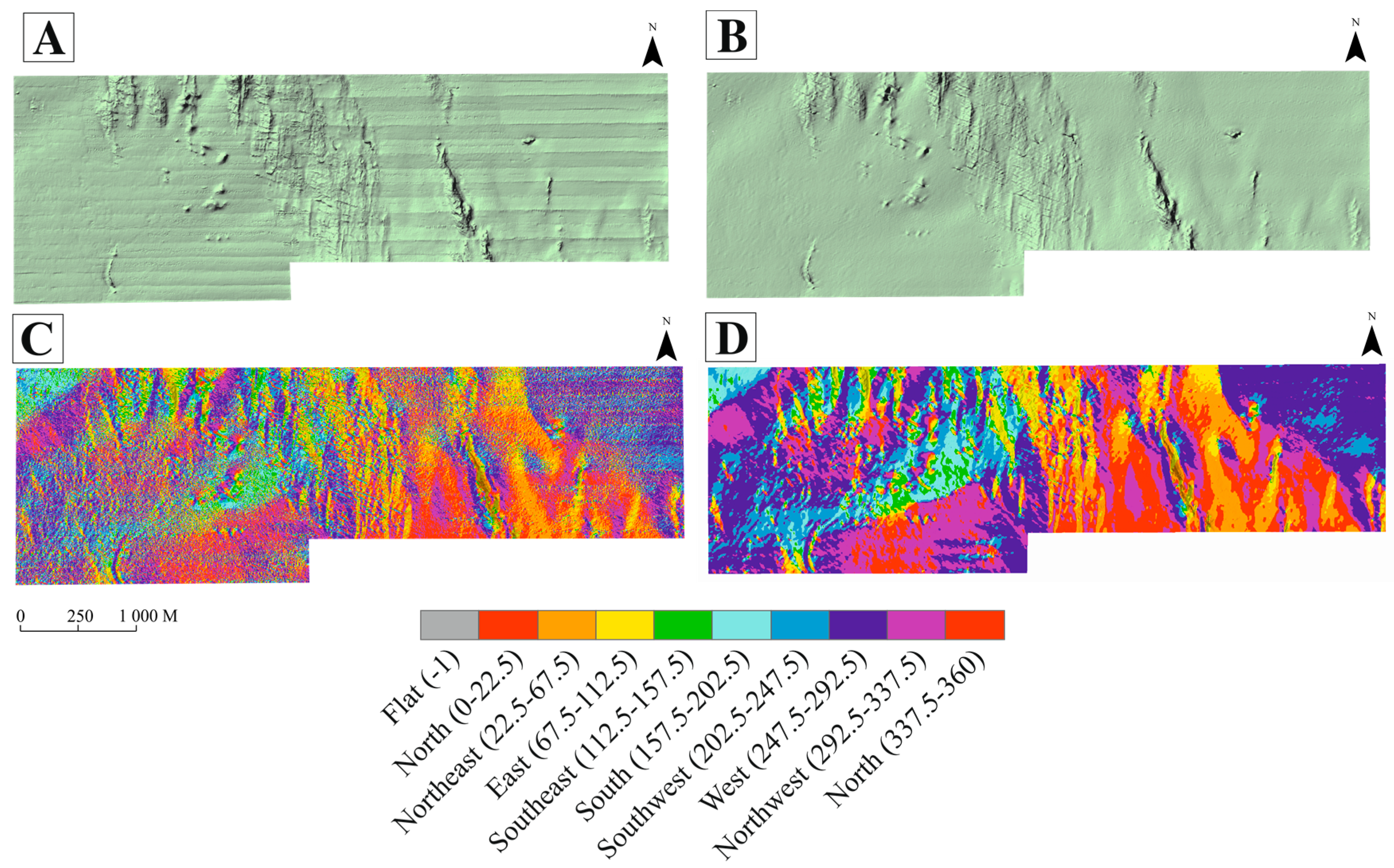
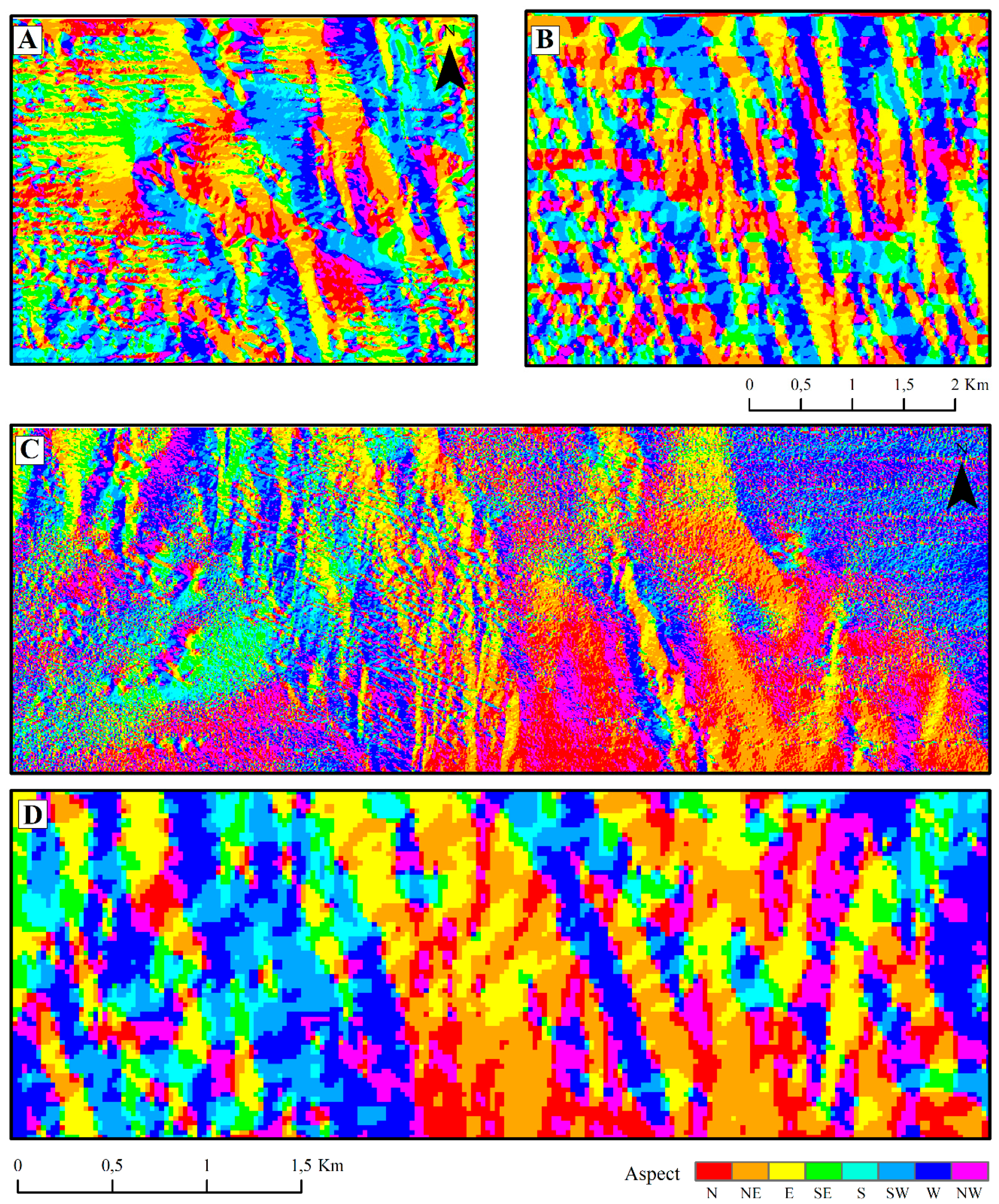
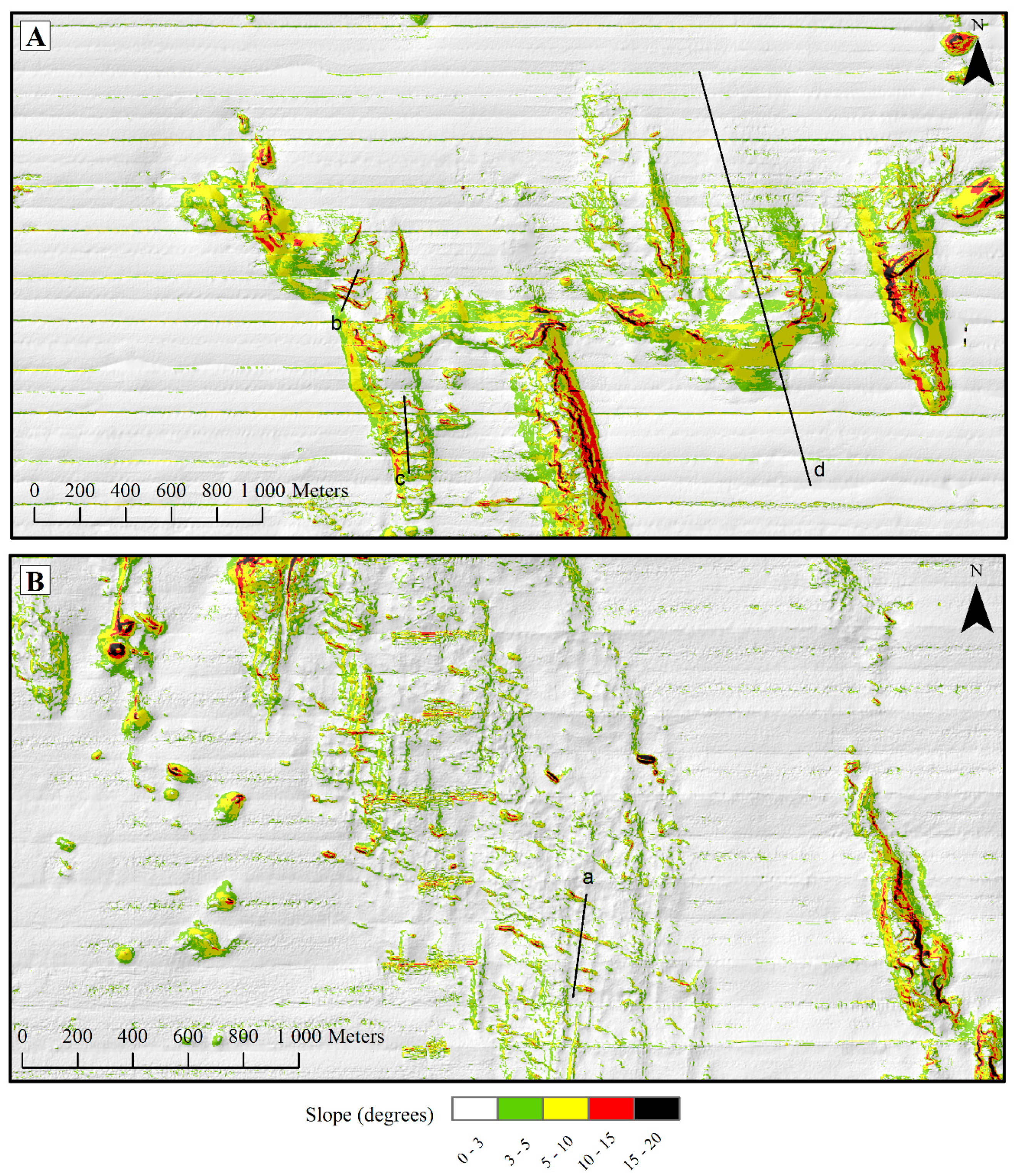
2.5. GIS Analyses of Bottom Relief
SBP Data Processing
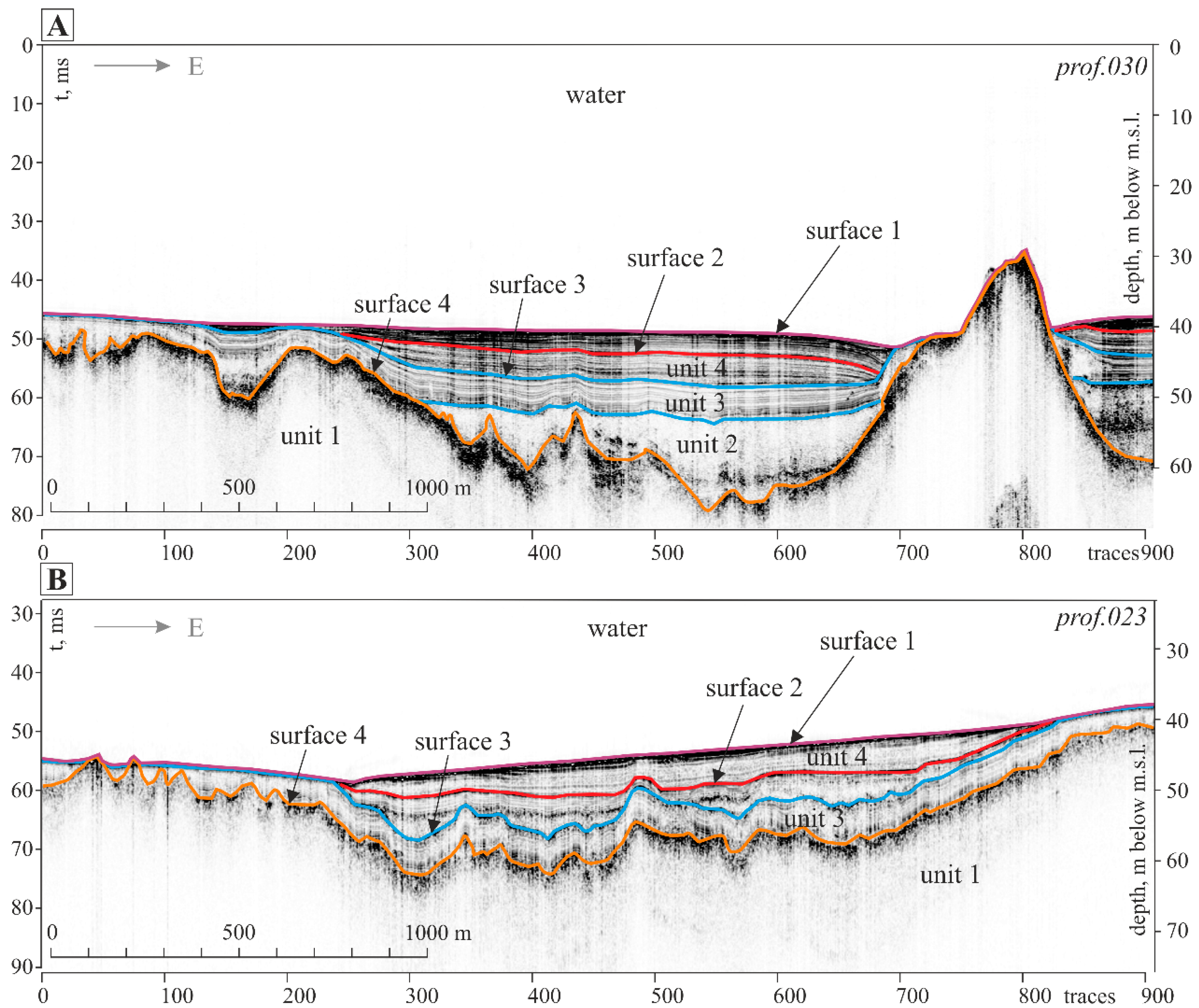
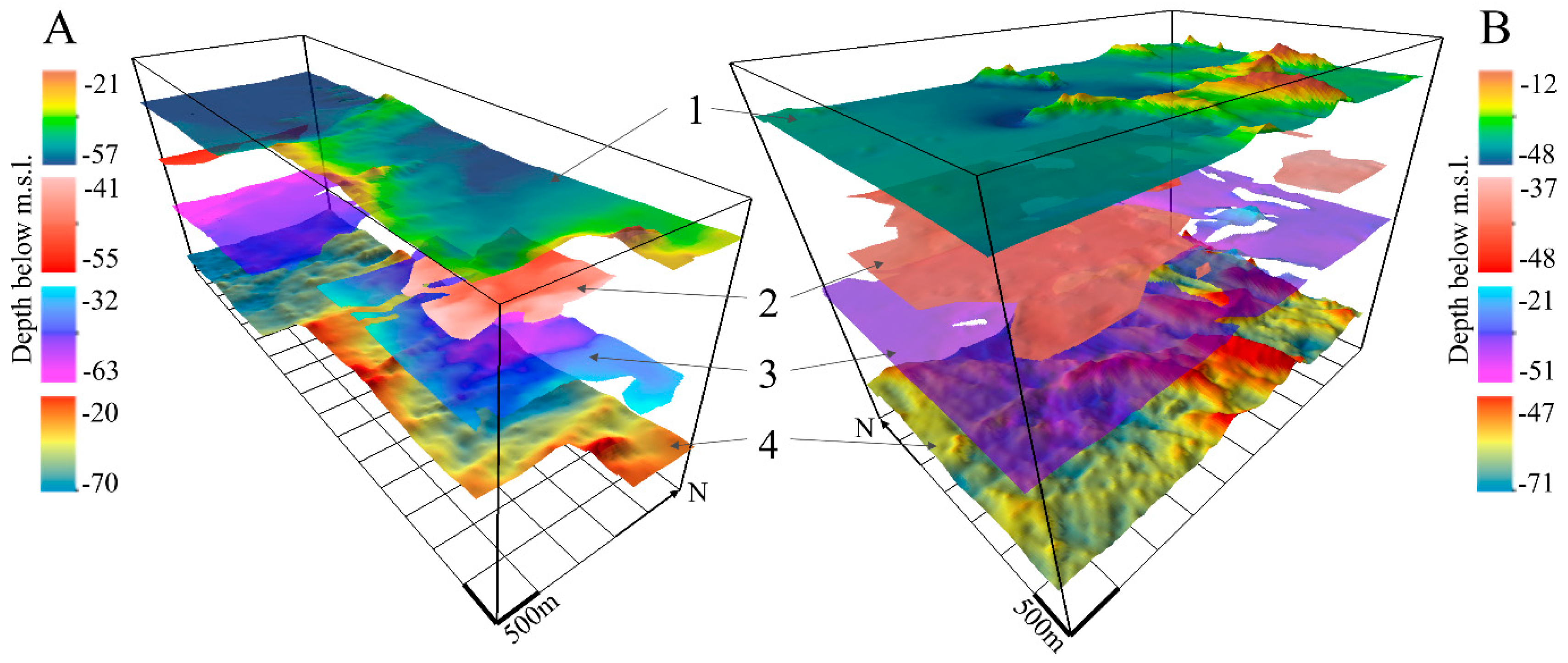
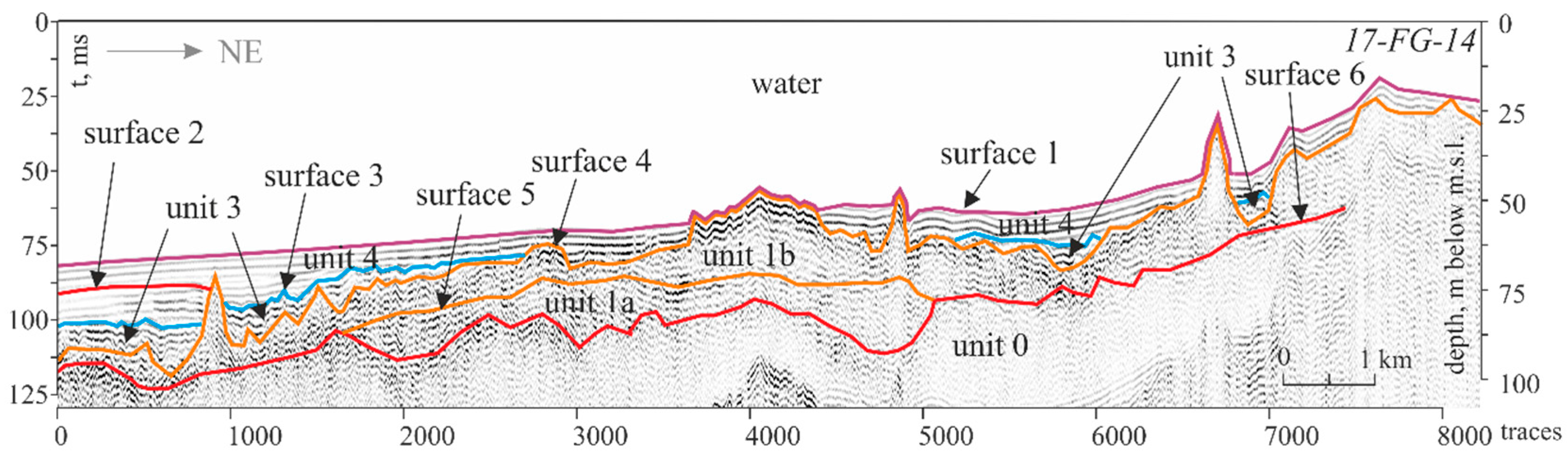
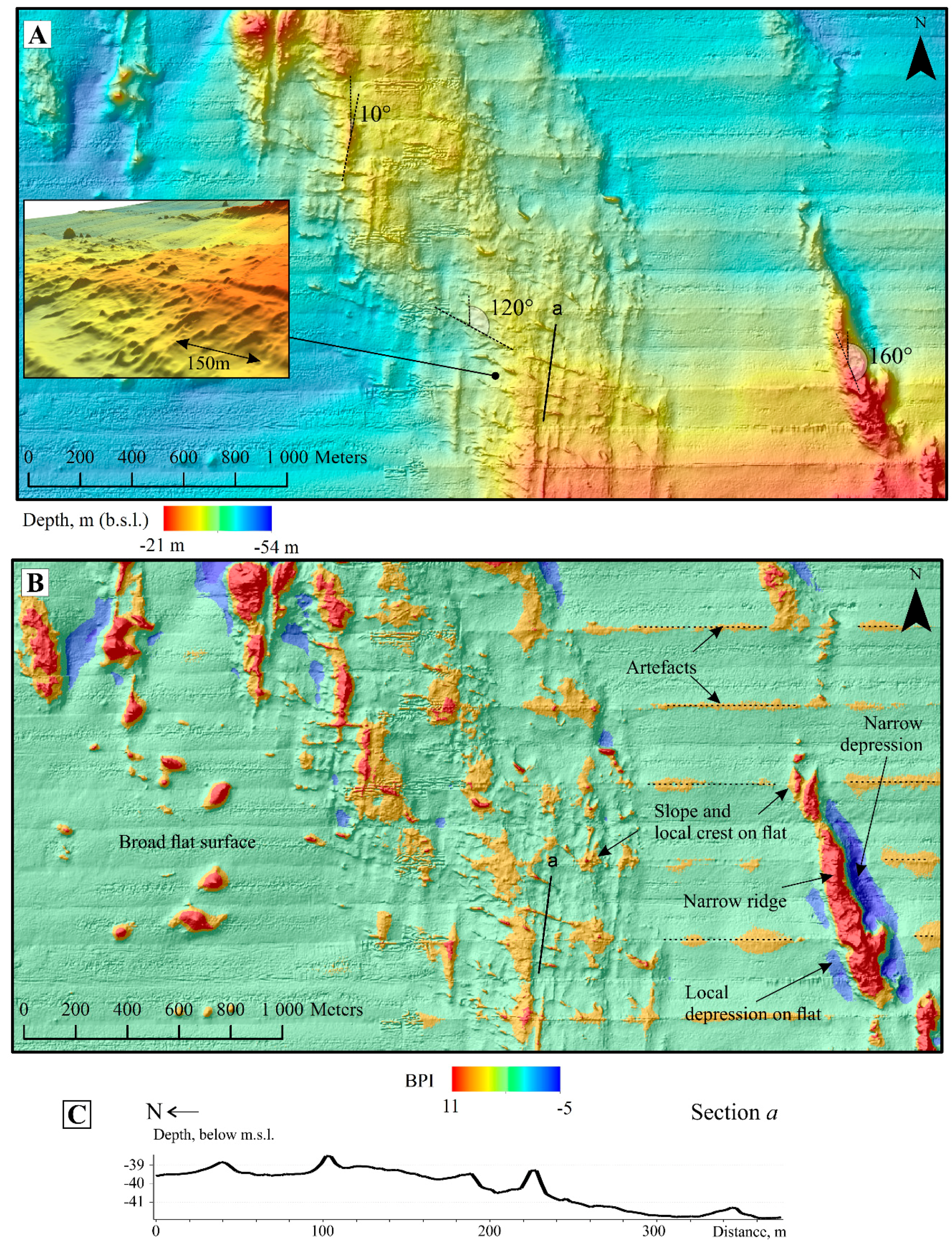
3. Results
4. Discussion
5. Conclusions
- Geophysical research in key areas of Vyborg Bay and north of Moschny Island using high-resolution MBES and SBP data revealed, for the first time, well-defined streamlined moraine ridges, De Geer moraines, and end-moraine ridges. Mapping of these glacial features established the location and orientation of the ice sheet margins during different stages of deglaciation in the Eastern (Russian) Gulf of Finland.
- Our interpretations of high-resolution seismic-reflection profiles and 3D models of the till surfaces, Late Pleistocene sediments, and the mapping of the modern seafloor relief indicate that a significant fall in the water level in the Early Holocene and that, most likely, several water-level fluctuations occurred, documented by erosion surfaces (acoustic unconformable horizons) in silty-clay mud.
- We conclude that the distribution and thickness of Holocene silty-clay mud mapped within our study areas indicates a drastic change in sedimentation since the beginning of the Ancylus Lake stage. Since the Ancylus, accumulation occurred within local sedimentary basins, while conditions of large bottom areas of the Gulf of Finland remained starved of sediment or suffered from erosion. Modern silty-clay accumulation in the Eastern Gulf of Finland occurs in local sedimentary basins, located at depths from 5 to 6 m in Neva Bay, to 80 m south of Gogland Island, which are separated by vast sediment starved and/or erosional areas.
Acknowledgments
Author Contributions
Conflicts of Interest
References
- Harff, J.; Björck, S.; Hoth, P. The Baltic Sea Basin: Introduction. The Baltic Sea Basin Central and Eastern European Development Studies (CEEDES); Springer: Berlin/Heidelberg, Germany, 2011; pp. 3–9. [Google Scholar]
- Uścinowicz, S. Geochemistry of the Baltic Sea Surface Sediments; Polish Geological Institute—National Research Institute: Warsaw, Poland, 2011; p. 356. ISBN 978-83-7538-814-5. [Google Scholar]
- Kaskela, A.; Rousi, H.; Ronkainen, M.; Orlova, M.; Babin, A.; Gogoberidze, G.; Kostamo, K.; Kotilainen, A.; Neevin, I.; Ryabchuk, D.; et al. Linkages between benthic assemblages and physical environmental factors: The role of geodiversity in Eastern Gulf of Finland ecosystems. Cont. Shelf Res. 2017, 142, 1–13. [Google Scholar] [CrossRef]
- Uścinowicz, S. Relative Sea Level Changes, Glacio-Isostatic Rebound and Shoreline Displacement in the Southern Baltic; Polish Geological Institute: Warsaw, Poland, 2003; Volume 10, p. 79. [Google Scholar]
- Lampe, R.; Meter, H.; Ziekur, R.; Janke, W.; Endtmann, E. Holocene Evolution of the Irregularly Sinking Baltic Sea Coast and the Interactions of the Sea-Level Rise, Accumulation Space and Sediment Supply. In SINCOS–Sinking Coasts. Geosphere, Ecosphere and Anthroposhere of the Holocene Southern Baltic Sea; Harff, J., Luth, F., Eds.; Bericht der Romisch-Germanischen Kommission; Philipp von Zabern: Darmstadt, Germany, 2007; pp. 15–46. [Google Scholar]
- Harff, J.; Meyer, M. Coastlines of the Baltic Sea–Zones of Competition Between Geological Processes and a Changing Climate: Examples from the Southern Baltic; The Baltic Sea Basin Central and Eastern European Development Studies (CEEDES) Book Series; Springer: Berlin/Heidelberg, Germany, 2011; pp. 149–164. [Google Scholar]
- Hyttinen, O.; Kotilainen, A.T.; Virtasalo, J.J.; Kekäläinen, P.; Snowball, I.; Obrochta, S.; Andrén, T. Holocene stratigraphy of the Ångermanälven River estuary, Bothnian Sea. Geo-Mar. Lett. 2016, 37, 273–288. [Google Scholar] [CrossRef]
- Gordeeva, S.; Malinin, V. Gulf of Finland Sea Level Variability; RSHU Publishers: St. Petersburg, Russia, 2014; p. 179. ISBN 978-5-86813-403-6. (In Russian) [Google Scholar]
- Rosentau, A.; Veski, S.; Kriiska, A.; Aunap, R.; Vassiljev, J.; Saarse, L.; Hang, T.; Heinsalu, A.; Oja, T. Palaeogeographic Model for the SW Estonian Coastal Zone of the Baltic Sea; The Baltic Sea Basin Central and Eastern European Development Studies (CEEDES) book series; Springer: Berlin/Heidelberg, Germany, 2011; pp. 165–188. [Google Scholar]
- Rosentau, A.; Muru, M.; Kriiska, A.; Subetto, D.A.; Vassiljev, J.; Hang, T.; Gerasimov, D.; Nordqvist, K.; Ludikova, A.; Lõugas, L.; et al. Stone Age settlement and Holocene shore displacement in the Narva-Luga Klint Bay area, eastern Gulf of Finland. Boreas 2013, 42, 912–931. [Google Scholar] [CrossRef]
- Sandgren, P.; Subetto, D.A.; Berglund, B.E.; Davydova, N.N.; Savelieva, L.A. Mid-Holocene Littorina Sea transgressions based on stratígraphíc studies in coastal lakes of NW Russia. GFF 2004, 126, 363–380. [Google Scholar] [CrossRef]
- Miettinen, A.; Savelieva, L.; Subetto, D.; Dzhinoridze, R.; Arslanov, K.; Hyvärinen, H. Palaeoenvironment of the Karelian Isthmus, the easternmost part of the Gulf of Finland, during the Litorina Sea stage of the Baltic Sea history. Boreas 2007, 36, 441–458. [Google Scholar] [CrossRef]
- Ryabchuk, D.; Zhamoida, V.; Amantov, A.; Sergeev, A.; Gusentsova, T.; Sorokin, P.; Kulkova, M.; Gerasimov, D. Development of the coastal systems of the easternmost Gulf of Finland, and their links with Neolithic–Bronze and Iron Age settlements. Geol. Soc. Lond. Spec. Publ. 2016, 411, 51–76. [Google Scholar] [CrossRef]
- Petrov, O.V. Atlas of Geological and Geoecological Maps of the Russian Part of the Baltic Sea; VSEGEI: St. Petersburg, Russia, 2010; 78p. [Google Scholar]
- Virtasalo, J.J.; Ryabchuk, D.; Kotilainen, A.T.; Zhamoida, V.; Grigoriev, A.; Sivkov, V.; Dorokhova, E. Middle Holocene to present sedimentary environment in the easternmost Gulf of Finland (Baltic Sea) and the birth of the Neva River. Mar. Geol. 2014, 350, 84–96. [Google Scholar] [CrossRef]
- Ryabchuk, D.; Hyttinen, O.; Zhamoida, V.; Kotilainen, A.; Sergeev, A.; Amantov, A.; Budanov, L.; Moskovtsev, A. Deglaciation of the Eastern Gulf of Finland basin. Unpublished manuscript. 2017. [Google Scholar]
- Krasnov, I.I.; Duphorn, K.; Voges, A. (Eds.) International Quaternary Map of Europe 1:2,500,000; Sheet 3, Nordkapp; UNESCO: Hanover, Germany, 1971. [Google Scholar]
- Zarina, E.P. Geochronology and Paleogeography of Late Pleistocene of the North-West of Russia. In Periodization and Paleogeography of Late Pleistocene; VSEGEI: Leningrad, Soviet Union, 1970; pp. 27–33. (In Russian) [Google Scholar]
- Kvasov, D.D. Late Quaternary History of the Large Lakes and Inner Seas of the Eastern Europe; Nauka: Leningrad, Russia, 1975; p. 278. (In Russian) [Google Scholar]
- Raukas, A.; Hyvärinen, H. (Eds.) Geology of the Gulf of Finland; Valgus: Tallinn, Estonia, 1991; p. 422. [Google Scholar]
- Subetto, D.A. Lake Sediments: Paleolimnological Reconstructions; Herzen Russian State Pedagogical University: St. Petersburg, Russia, 2009; p. 339. ISBN 978-5-8064-1444-2. (In Russian, resume in English). [Google Scholar]
- Vassiljev, J.C.B.C.; Saarse, L.; Rosentau, A. Palaeoreconstruction of the Baltic Ice Lake in the Eastern Baltic; The Baltic Sea Basin Central and Eastern European Development Studies (CEEDES) Book Series; Springer: Berlin/Heidelberg, Germany, 2011; pp. 189–202. [Google Scholar]
- Hughes, A.L.C.; Gyllencreutz, R.; Lohne, Ø.S.; Mangerud, J.; Svendsen, J.I. The last Eurasian ice sheets — A chronological database and time-Slice reconstruction, DATED-1. Boreas 2016, 45, 1–45. [Google Scholar] [CrossRef] [Green Version]
- Dorschel, B.; Wheeler, A.J.; Monteys, X.; Verbruggen, K. On the Irish Seabed. Atlas of the Deep-Water Seabed; Springer: New York, NY, USA, 2010; p. 164. [Google Scholar]
- Harris, P.T.; Baker, E.K. GeoHab Atlas of Seafloor Geomorphic Features and Benthic Habitats. Seafloor Geomorphology as Benthic Habitat; Elsevier: Amsterdam, Netherlands, 2012; pp. 871–890. [Google Scholar]
- Diesing, M.; Green, S.L.; Stephens, D.; Lark, R.M.; Stewart, H.A.; Dove, D. Mapping seabed sediments: Comparison of manual, geostatistical, object-based image analysis and machine learning approaches. Cont. Shelf Res. 2014, 84, 107–119. [Google Scholar] [CrossRef] [Green Version]
- Dove, D.; Arosio, R.; Finlayson, A.; Bradwell, T.; Howe, J.A. Submarine glacial landforms record Late Pleistocene ice-Sheet dynamics, Inner Hebrides, Scotland. Quat. Sci. Rev. 2015, 123, 76–90. [Google Scholar] [CrossRef] [Green Version]
- Lecours, V.; Dolan, M.F.J.; Micallef, A.; Lucieer, V.L. A review of marine geomorphometry, the quantitative study of the seafloor. Hydrol. Earth Syst. Sci. 2016, 20, 3207–3244. [Google Scholar] [CrossRef]
- Flemming, N.C.; Harff, J.; Moura, D.; Burgess, A.; Bailey, G.N. (Eds.) Submerged Landscapes of the European Continental Shelf; John Wiley & Sons, Inc.: Hoboken, NJ, USA, 2017; p. 533. ISBN 9781118922132. [Google Scholar]
- Petrov, O.V.; Lygin, A.M. (Eds.) Information Bulletin on Geological Environment Assessment of the Near-Shore Areas of the Barents, White and Baltic Seas; VSEGEI: St. Petersburg, Russia, 2014; p. 136. (In Russian) [Google Scholar]
- Raateoja, M.; Setälä, O. The Gulf of Finland Assessment; Reports of the Finnish Institute Series; Finnish Environment Institute: Helsinki, Finland, 2016; Volume 27, p. 363. [Google Scholar]
- Zhamoida, V.; Grigoriev, A.; Ryabchuk, D.; Evdokimenko, A.; Kotilainen, A.T.; Vallius, H.; Kaskela, A.M. Ferromanganese concretions of the eastern Gulf of Finland–Environmental role and effects of submarine mining. J. Mar. Syst. 2017, 172, 178–187. [Google Scholar] [CrossRef]
- Sibson, R. Chapter 2: A Brief Description of Natural Neighbor Interpolation. In Interpolating Multivariate Data; John Wiley & Sons: New York, NY, USA, 1981; pp. 21–36. [Google Scholar]
- Demyanov, V.; Savelyeva, E. Geostatistics: Theory and Practice; Nauka: Moscow, Russia, 2010; p. 327. ISBN 978-5-02-037478-2. [Google Scholar]
- Oimoen, M.J. An Effective Filter for Removal of Production Artifacts in U.S. Geological Survey 7.5-Minute Digital Elevation Models. In Proceedings of the Fourteenth International Conference on Applied Geologic Remote Sensing, Las Vegas, NV, USA, 6–8 November 2000; pp. 311–319. [Google Scholar]
- Peregro, A. SRTM DEM Destriping with SAGA GIS: Consequences on Drainage Network Extraction. Available online: http://www.webalice.it/alper78/saga_mod/destriping/destriping.html (accessed on 7 December 2017).
- Wright, D.J.; Lundblad, E.R.; Larkin, E.M.; Rinehart, R.W.; Murphy, J.; Cary-Kothera, L.; Draganov, K. ArcGIS Benthic Terrain Modeler. Available online: http://www.csc.noaa.gov/products/btm/ (accessed on 20 January 2017).
- Lundblad, E.; Wright, D.J.; Miller, J.; Larkin, E.M.; Rinehart, R.; Battista, T.; Anderson, S.M.; Naar, D.F.; Donahue, B.T. A benthic terrain classification scheme for American Samoa. Mar. Geod. 2006, 29, 89–111. [Google Scholar] [CrossRef]
- Bulletin de la Commission Pour L’etude du Quaternaire. Available online: http://ginras.ru/library/pdf/2_1930_bull_quatern_comission.pdf (accessed on 10 November 2017).
- Donner, J. The Quaternary History of Scandinavia; Cambridge University Press: London, UK, 1995; p. 200. ISBN 978-0-521-01831-9. [Google Scholar]
- Saarnisto, M.; Saarinen, T. Deglaciation chronology of the Scandinavian Ice Sheet from the Lake Onega Basin to the Salpausselkä End Moraines. Glob. Planet. Chang. 2001, 31, 387–405. [Google Scholar] [CrossRef]
- Hang, T. A local clay-Varve chronology and proglacial sedimentary environment in glacial Lake Peipsi, eastern Estonia. Boreas 2003, 32, 416–426. [Google Scholar] [CrossRef]
- Kalm, V. Pleistocene chronostratigraphy in Estonia, southeastern sector of the Scandinavian glaciation. Quat. Sci. Rev. 2006, 25, 960–975. [Google Scholar] [CrossRef]
- Vassiljev, J.; Saarse, L. Timing of the Baltic Ice Lake in the eastern Baltic. Bull. Geol. Soc. Finl. 2013, 85, 9–18. [Google Scholar] [CrossRef]
- Breilin, O.; Kotilainen, A.; Nenonen, K.; Virransalo, P.; Ojalainen, J.; Stén, C.-G. Geology of the Kvarken Archipelago. Appendix 1 to the application for nomination of the Kvarken Archipelago to the World Heritage list. In Metsähallitus Western Finland Natural Heritage Services, West Finland Regional Environment Centre; Regional Council of Ostrobothnia: Vaasa, Finland, 2004; p. 12. [Google Scholar]
- Breilin, O.; Kotilainen, A.; Nenonen, K.; Räsänen, M. The unique moraine morphology, stratotypes and ongoing geological processes at the Kvarken Archipelago on the land uplift area in the western coast of Finland. In Quaternary Studies in the Northern and Arctic Regions of Finland, Proceedings of the Workshop Organized within the Finnish National Committee for Quaternary Research (INQUA), Kilpisjärvi Biological Station, Finland, 13–14 January 2005; Ojala, A.E.K., Ed.; Special Paper 40; Geological Survey of Finland: Espoo, Finland, 2005; pp. 97–111. [Google Scholar]
- Kotilainen, A.T.; Kaskela, A.M. Comparison of airborne LiDAR and shipboard acoustic data in complex shallow water environments: Filling in the white ribbon zone. Mar. Geol. 2017, 385, 250–259. [Google Scholar] [CrossRef]
- Karukäpp, R.; Raukas, A. Deglaciation History. In Geology and Mineral Resources of Estonia; Raukas, A., Teedumäe, A., Eds.; Estonian Academy Publishers: Tallinn, Estonia, 1997; pp. 263–267. ISBN 9985-50-185-3. [Google Scholar]
- Talviste, P.; Hang, T.; Kohv, M. Glacial varves at the distal slope of Pandivere-Neva ice-Recessional formations in western Estonia. Bull. Geol. Soc. Finl. 2012, 84, 7–19. [Google Scholar] [CrossRef]
- Glückert, G. The First Salpausselkä at Lohja, southern Finland. Bull. Geol. Soc. Finl. 1986, 58, 45–55. [Google Scholar] [CrossRef]
- Donner, J. The Younger Dryas age of the Salpausselkä moraines in Finland. Bull. Geol. Soc. Finl. 2010, 82, 69–80. [Google Scholar] [CrossRef]
- Uścinowicz, S. Moreny De Geera na Ławicy Slupskiej-nowe dowody na subakwalną deglacjację obszaru południowego Bałtyku. In Proceedings of the XVIII Konferencja Naukowo-Szkoleniowa. Stratigrafia Plejstocenu Polski, Stara Kiszewa, Poland, 5–9 January 2011. (In Polish). [Google Scholar]
- Todd, B.J. De Geer moraines on German Bank, southern Scotian Shelf of Atlantic Canada. Geological Society, London, UK. Memoirs 2016, 46, 259–260. [Google Scholar] [CrossRef]
- Bradwell, T.; Stoker, M.S.; Golledge, N.R.; Wilson, C.K.; Merritt, J.W.; Long, D.; Everest, J.D.; Hestvik, O.B.; Stevenson, A.G.; Hubbard, A.L.; et al. The northern sector of the last British Ice Sheet: Maximum extent and demise. Earth-Sci. Rev. 2008, 88, 207–226. [Google Scholar] [CrossRef] [Green Version]
- Amantov, A.V.; Amantova, M.V. Modeling of postglacial development of Lake Ladoga and eastern part of the Gulf of Finland. Reg. Geol. Metallog. 2017, 69, 5–14. (In Russian) [Google Scholar]
- Spiridonov, M.; Ryabchuk, D.; Kotilainen, A.; Vallius, H.; Nesterova, E.; Zhamoida, V. The Quaternary deposits of the Eastern Gulf of Finland. In Holocene Sedimentary Environment and Sediment Geochemistry of the Eastern Gulf of Finland, Baltic Sea; Vallius, H., Ed.; Geological Survey of Finland: Espoo, Finland, 2007; pp. 5–18. ISBN 978-951-69-09-953. [Google Scholar]
- Amantov, A.V.; Zhamoida, V.A.; Ryabchuk, D.V.; Spiridonov, M.A.; Sapelko, T.V. Geological structure of submarine terraces of the eastern Gulf of Finland and modeling of their development during postglacial time. Reg. Geol. Metallog. 2012, 50, 5–27. (In Russian) [Google Scholar]
- Amantov, A.; Ryabchuk, D.; Fjeldskaar, W.; Zhamoida, V.; Amantova, M. Possible role of Hydroisostasy in Peculiarities of Late Glacial-Postglacial Sedimentation of the Eastern part of the Gulf of Finland and Lake Ladoga. In EGU General Assembly, Geophysical Research Abstracts; EGU General Assembly: Vienna, Austria, 2013; Volume 15. [Google Scholar]
- Sergeev, A.; Ryabchuk, D.; Gusentsova, T.; Sorokin, P.; Nesterova, E.; Zhamoida, V.; Spiridonov, M.; Kulkova, M.; Glukhov, V. Reconstruction of the paleorelief of the Littorina Sea coastal zone within St. Petersburg based on a study of the archaeological site Okhta 1.59. Ger. Anz. Romis.-Ger. Kom. Deutsch. Archaologischen Inst. 2014, 92, 33–59. [Google Scholar]


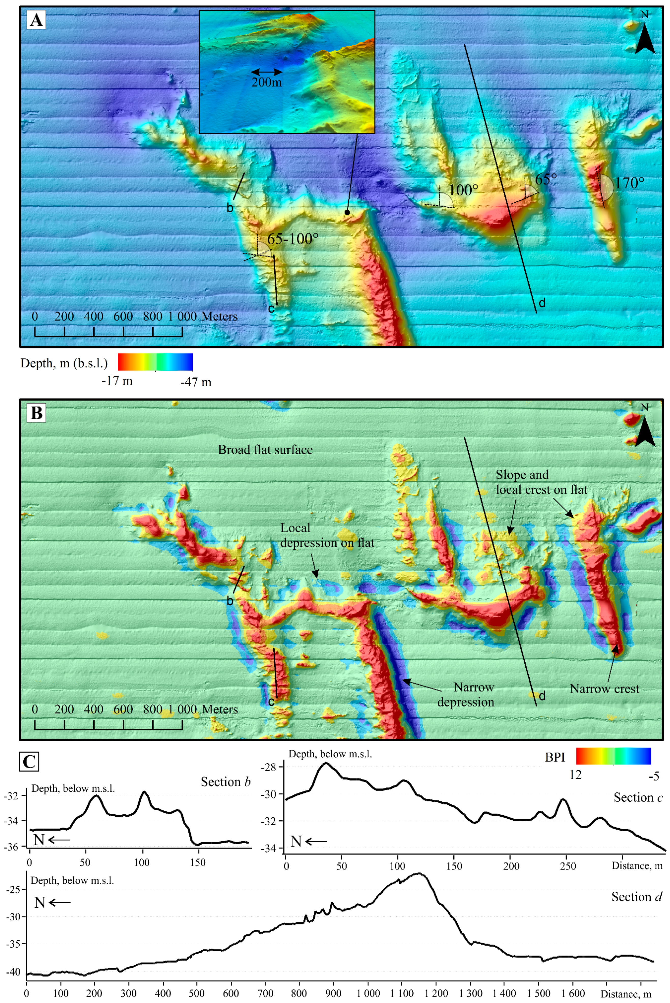
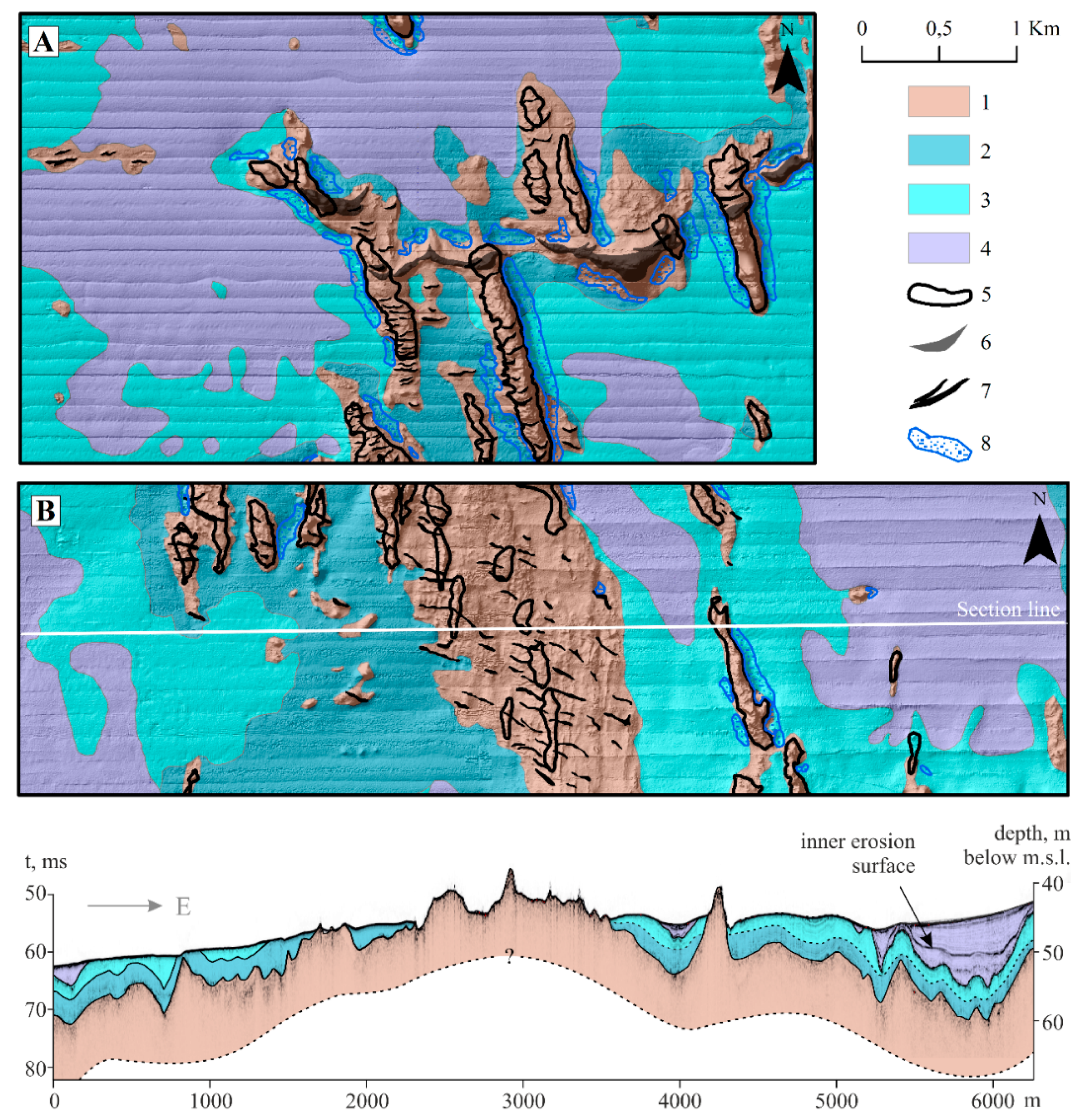
| Location | Shape | Direction (Azimuth) | Height Above Around Seafloor, m | Height of Ridge Above Its Base, m | Width of Ridge Base, m | Length of Ridge, m | Slope, Degrees | Crests Interval, m | Geological Interpretation |
|---|---|---|---|---|---|---|---|---|---|
| Isl. Moschny | Linear | NNE–SSW (10°) | 0.5–1 | - | 20–60 | 1200 | 1–3° | - | Glacial erosion ridges |
| Linear | SSE–NNW (160°) | 5–8 | 15–20 | 100 | 1000 | 5–20° | - | Streamlined moraine ridges | |
| Linear | SE–NW (120°) | 0.5–1.5 | 1–2 | 8–10 | 1300 | 5–15° | 50–150 (av.85) | De Geer moraine | |
| Vyborg Bay | Linear | SSE–NNW (170°) | 10–15 | 15–20 | 130–170 | 1000 | 5–20° | - | Streamlined moraine ridges |
| Crescent | NE–SW and SE–NW (65° and 100°) | 10–20 | 10–25 | from 70–200 to 300–1000 | more than 4300 | 3–4° N slope 10° S slope | - | End-moraine ridges | |
| Crescent | NE–SW and SE–NW (65° and 100°) | 0.5–1.5 | 1–2 | 8–10 | 300 | 5–20° | 50 | De Geer moraine |
© 2018 by the authors. Licensee MDPI, Basel, Switzerland. This article is an open access article distributed under the terms and conditions of the Creative Commons Attribution (CC BY) license (http://creativecommons.org/licenses/by/4.0/).
Share and Cite
Ryabchuk, D.; Sergeev, A.; Krek, A.; Kapustina, M.; Tkacheva, E.; Zhamoida, V.; Budanov, L.; Moskovtsev, A.; Danchenkov, A. Geomorphology and Late Pleistocene–Holocene Sedimentary Processes of the Eastern Gulf of Finland. Geosciences 2018, 8, 102. https://doi.org/10.3390/geosciences8030102
Ryabchuk D, Sergeev A, Krek A, Kapustina M, Tkacheva E, Zhamoida V, Budanov L, Moskovtsev A, Danchenkov A. Geomorphology and Late Pleistocene–Holocene Sedimentary Processes of the Eastern Gulf of Finland. Geosciences. 2018; 8(3):102. https://doi.org/10.3390/geosciences8030102
Chicago/Turabian StyleRyabchuk, Daria, Alexander Sergeev, Alexander Krek, Maria Kapustina, Elena Tkacheva, Vladimir Zhamoida, Leonid Budanov, Alexandr Moskovtsev, and Aleksandr Danchenkov. 2018. "Geomorphology and Late Pleistocene–Holocene Sedimentary Processes of the Eastern Gulf of Finland" Geosciences 8, no. 3: 102. https://doi.org/10.3390/geosciences8030102
APA StyleRyabchuk, D., Sergeev, A., Krek, A., Kapustina, M., Tkacheva, E., Zhamoida, V., Budanov, L., Moskovtsev, A., & Danchenkov, A. (2018). Geomorphology and Late Pleistocene–Holocene Sedimentary Processes of the Eastern Gulf of Finland. Geosciences, 8(3), 102. https://doi.org/10.3390/geosciences8030102