Article

Numerical Modeling of Remediation Scenarios of a Groundwater Cr(VI) Plume in an Alpine Valley Aquifer

Department of Earth and Environmental Sciences, University of Milano-Bicocca, Piazza della Scienza 1, 20126 Milan, Italy
*
Author to whom correspondence should be addressed.
Geosciences 2018, 8(6), 209; https://doi.org/10.3390/geosciences8060209
Submission received: 3 May 2018 / Revised: 6 June 2018 / Accepted: 7 June 2018 / Published: 8 June 2018
(This article belongs to the Special Issue Groundwater Pollution)

Abstract

:
This work presents the numerical modeling of remediation scenarios aimed at containing and attenuating the groundwater pollution by Cr(VI) sourced from a steelworks area that affects the Alpine aquifer system in the Aosta Plain (N Italy). Here, groundwater is used for drinking water supply and food and beverage production, so the adoption of remediation works is urgently needed. More specifically, three remediation scenarios were modeled using MODFLOW-2000 and MT3DMS: (a) the activation of a hydraulic barrier to contain the pollution within the source area (Scenario 1); (b) the removal of the pollution sources and the natural attenuation of the residual groundwater plume (Scenario 2); and (c) a combination of the previous two works (Scenario 3). Model results for Scenario 1 showed that a hydraulic barrier composed of five wells located along the eastern border of the steelworks area would contain Cr(VI) concentrations above 5 µg/L (i.e., the Italian regulatory limit) within the steelworks area; the barrier would have a total discharge of 27,500 m3/day, which could be compensated by the deactivation of three steelworks wells; the hydraulic barrier would drop the Cr(VI) concentrations below 5 µg/L in the areas downstream of the steelworks after ~3 years from its start of operation. Results for Scenario 2 highlighted that the removal of the Cr(VI) sources would drop the Cr(VI) concentrations below 5 µg/L in the areas downstream of the steelworks after ~2.5 years, and lead to a full remediation of the Cr(VI) groundwater plume (i.e., total Cr(VI) mass in the aquifer close to zero) after 17 years. Results for Scenario 3 showed that the removal of the Cr(VI) sources accompanied by the activation of the hydraulic barrier would led to a faster remediation within the first 14 years from the starting of the remediation works, with concentrations below 5 µg/L in the areas downstream of the steelworks obtained after ~2.3 years.

1. Introduction

The use of numerical models to support the management of groundwater resources is increasing in the last decades. Groundwater flow and contaminant transport models can represent a valid decision support tool for handling a variety of problems in hydrogeology, ranging from the depletion of groundwater resources to groundwater quality concerns. The implementation of numerical modeling allows for the joint consideration of several aspects that could have different weights on the evaluation of the quantity and quality of groundwater resources. Overall, groundwater models provide the chance, on one hand, to improve the comprehension of the behavior of the hydrogeological system and, on the other hand, to implement more suitable management policies for groundwater resources.
One of the most used codes for simulating 3D groundwater flow in hydrogeology studies is MODFLOW (McDonald & Harbaugh [1] and successive versions), which uses a various number of packages to simulate the different elements of the hydrogeological system (e.g., river, drain, pumping well, no-flow zone, etc.) and their mutual relationships. Furthermore, many other MODFLOW-related codes exist for evaluating a large variety of aspects related to groundwater. For example, the MODPATH code [2] allows tracking of the advective component of the groundwater flow, the MT3DMS code [3] is able to simulate the fate of dissolved contaminants, taking into account the advective-dispersive transport equation together with some basilar physicochemical reactions, whereas the SEAWAT [4] code is able to simulate variable density groundwater flow, therefore allowing one to deal with saltwater intrusion and related problems.
Many recent works [5,6,7,8,9,10] reported the implementation of flow and transport models through the family of MODFLOW-related codes, in order to support the management of groundwater resources and environmental problems. Along these lines, the present study involves the numerical modeling of remediation scenarios of the hexavalent chromium (Cr(VI)) plume in the aquifer system of the Aosta Plain (N Italy) using MODFLOW-related codes. Many works reporting the modeling of transport and remediation works of Cr(VI) groundwater pollution exist in the literature [11,12,13,14,15,16,17,18,19]. The main aim here is to present some examples of operations that could be done for remediating the Cr(VI) pollution in order to improve the groundwater quality and protect the health of the population living in the area. Indeed, the Cr(VI) is a carcinogenic species, and its concentration in groundwater should be kept as low as possible. Moreover, groundwater in the Aosta Plain is used to fulfill many human needs, such as drinking water supply and production of food and beverage. The need of an urgent remediation of the Cr(VI) pollution in the aquifer of the Aosta Plain is also highlighted by the recent work by Tiwari and De Maio [20] that assessed a high potential cancer risk for the local population related to the Cr(VI) groundwater pollution.

2. Materials and Methods
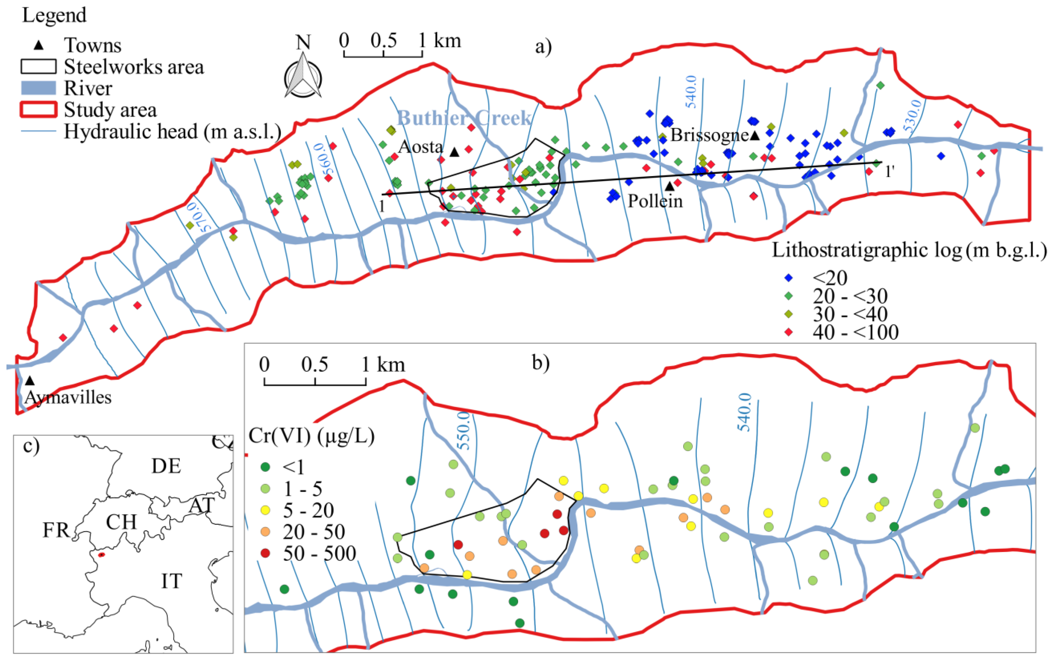
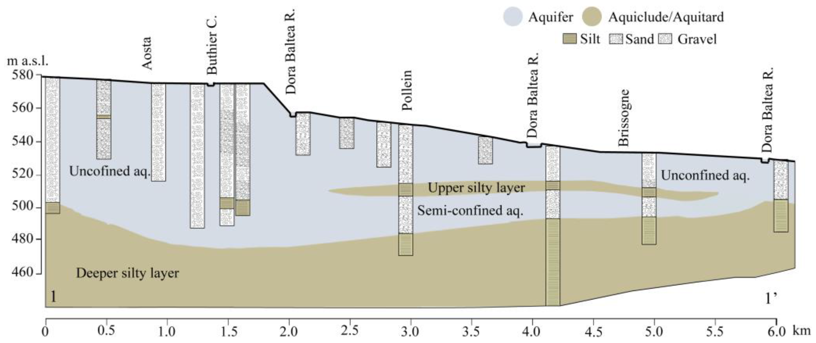
2.1. Study Area

The present work is referred to the aquifer system of the Aosta Plain, located within the Aosta Valley Region, NW Italy (Figure 1). More precisely, the study area covers ~30 km2 around the town of Aosta, between the villages of Aymavilles and Brissogne, and it is crossed from west to east by the Dora Baltea River (Figure 1a). Within the study area, this river collects water from 14 tributaries, among which the most important is the Buthier Creek, which crosses the town of Aosta from north to south (Figure 1a). The geological and hydrogeological features of this area were exhaustively described by many previous studies [20,21,22,23,24,25,26,27,28,29,30], so only a brief summary is given in the following. The aquifer system is formed by fluvioglacial, alluvial, lacustrine, and fan deposits, which overlay a deep crystalline basement. The exploited unconfined aquifer has a thickness of ~85–90 m; in the eastern part of the area, the thickness decreases up to 50 m, and the aquifer is subdivided by a silty layer located at around 20 m b.g.l., into a shallower unconfined and a deeper semi-confined aquifer (Figure 2). The aquifer system is recharged by ice and snow melt, precipitation, and losing surface water bodies and discharges by well extraction, gaining surface water bodies, and downstream outflow. In particular, the Dora Baltea River plays an important role in the groundwater balance [27]: it is losing in the western part of the area, i.e., upstream of the town of Aosta, and becomes gaining moving downstream in the eastern part of the area. Groundwater flow is mainly directed from west to east with hydraulic heads and a hydraulic gradient that vary from ~580 to ~526 m a.s.l. and from 0.6 to 0.3 %, respectively (Figure 1a). Groundwater table depth ranges between 20 to 30 m b.g.l. in the western part of the study area, and 3–4 m b.g.l. in the eastern part, where the Dora Baltea River is gaining. Concerning the hydrochemistry, the groundwater has oxic conditions, and is mainly of the CaHCO3 type, with a shift toward the SO4–HCO3 type, due to the interaction with evaporites in the area south of the town of Aosta [24]. Furthermore, the studied aquifer is affected by Cr(VI) pollution, with concentrations up to ~440 µg/L [25] in the source area, which is a steelworks located in the southern part of the town of Aosta, that decreases 3.5 km downstream of the source area down to 1 µg/L (Figure 1b). The source of the Cr(VI) pollution is assumed to be the unsaturated zone beneath some areas of the steelworks used in the past years as open slag dumps, as the product of rainfall leaching, and accumulation in the unsaturated zone [21]; nowadays, the slag dumps were removed and those areas were subjected to capping to prevent rainwater infiltration and Cr(VI) leaching from the polluted unsaturated zone to groundwater. This Cr(VI) plume affects the groundwater quality of the whole aquifer system in the Aosta Plain so much that, according to the EU Water Framework Directive [31], its chemical status was assessed as poor [32].

2.2. Numerical Modeling

This work presents a 3D numerical modeling of some remediation works for containing and attenuating the Cr(VI) groundwater pollution in the study area using MODFLOW-2000 [33] and MT3DMS [3] through the graphical user interface Groundwater Vistas 6® (Environmental Simulations, Inc., Leesport, PA, USA). In particular, three scenarios were simulated:
  • Scenario 1—the simulation of a hydraulic barrier in order to contain the Cr(VI) plume within the area of the steelworks.
  • Scenario 2—the simulation of the natural attenuation of the dissolved Cr(VI) plume in groundwater after a complete removal of the Cr(VI) source from the unsaturated zone, by means of in situ or ex situ remediation, was achieved.
  • Scenario 3—a combination of the previous two remediation works.
The modeling of these scenarios is based on previous groundwater flow and Cr(VI) transport models [21,22]. The latter is hereafter called Scenario 0. Details on the settings and results of these previous models are described in the following subsections, together with the settings of the present models for simulating the remediation scenarios.

2.2.1. Groundwater Flow Modeling

The flow (and transport) model grid had 243 rows, 655 columns (uniform cell spacing of 20 m × 20 m) and 20 layers. The last 17 layers had a constant thickness of 5 m, whereas within the first three layers, the thickness can vary depending on the variation of the DEM that was used as top surface of layer 1. The 3D reconstruction of hydraulic conductivity (K) was made using geostatistics: the 176 lithologs from boreholes located in the Aosta Plain (Figure 1a) and stored in the TANGRAM database [34] were coded [35] and interpolated by kriging through a quasi-3D stratified approach [36] using GOCAD® (Emerson, St. Louis, MO, USA), as done in previous works [37,38]. The coding and attribution of K values made by TANGRAM were calibrated using eight previous pumping tests made in the study area [39,40], that led to K values for the unconfined sandy/gravelly aquifer ranging between 87.5 and 233.5 m/day; the calibration of the coding procedure led to attributing the K values of 432 m/day for well-sorted gravel and 57.6 m/day for well-sorted sand. The resulted 3D distribution of K values was then discretized into 10 zones; each zone was defined through the analysis of the frequency distribution of K. Finally, K values of each zone were adjusted during flow model calibration, leading to maximum and minimum values of 475 and 0.0864 m/day for Kx and Ky, and 47.5 and 0.00864 m/day for Kz, respectively [21]. The following boundary conditions were used [22]: (a) no flow (Neumann boundary condition) for reconstructing the “V” shape of the crystalline basement; (b) general head boundary (GHB; Cauchy boundary condition) for simulating the groundwater inflow and outflow through model margins at the western and eastern model edges, respectively; (c) recharge (Neumann boundary condition) through four zones with maximum and minimum values of 1.69 × 10⁻³ and 6.02 × 10⁻⁴ m/day [22]; these values were calculated as the water average surplus obtained by the Thornthwaite–Mather’s method, starting from the average monthly precipitation and temperature data; (d) Neumann boundary conditions through the multinode well (MNW) package for simulating the active wells in the area (i.e., 27 wells with ~63,000 m3/day of total discharge); (e) Cauchy boundary conditions through the streamflow-routing (SFR2) package [41] for simulating surface water bodies, in particular, the Dora Baltea River. Concerning the latter, since the SFR2 package is not supported by MT3DMS, before running the transport model, the SFR2 was substituted with the DRAIN package along the gaining segments of the Dora Baltea River. The flow model was run in steady-state conditions [22]. The flow model calibration was done by trial and error using 25 head and 1 flow targets, referred to January 2009, that can be considered as representative of average hydraulic conditions of the studied aquifer, since maximum and minimum hydraulic heads are registered during summer and spring, respectively [22]. The values of K and riverbed conductivity were the most sensitive, and they were adjusted in the calibration process.
The simulated heads in the area affected by the Cr(VI) plume are reported in Figure 3. Groundwater mainly flows from W to E with local perturbations due to well abstractions, particularly in and around the town of Aosta, and in the proximity of the steelworks. The hydraulic heads and groundwater table depths range from 554 m a.s.l. and 10–20 m b.g.l. just upstream of the steelworks, to 532 m a.s.l. and 3–4 m b.g.l. in the eastern part of the area, respectively; the gaining behavior of the Dora Baltea River can be clearly seen starting from the 540 m a.s.l. contour line and continues downstream. The error of the model mass balance was 0.0097%, and the scaled root mean square error was ~1% [21,22], highlighting the goodness of obtained fit.

2.2.2. Cr(VI) Transport Modeling (Scenario 0)

The transport model for Scenario 0 was based on the flow solution described in the previous section (Section 2.2.1). Concerning the setting of hydrodispersive and chemical parameters, effective porosity values were set through 10 zones, with the same extent of those used for discretizing K values, ranging between 0.05 and 0.28 [21]. The longitudinal dispersivity (αL) was 200 m; this value was calculated through the Mercado equation [42] considering the plume length of ~3500 m. The transversal (αT) and vertical dispersivity (αV) were 20 and 0.005 m, respectively. An equilibrium adsorption, represented by the Henry’s adsorption isotherm, was considered; the values for distribution coefficient (Kd), bulk density (ρb), and total porosity (n) were 0.05 L/kg, 1.7 g/cm3, and 0.3, respectively [21]. No degradation reactions were simulated, since Cr(VI) can be considered conservative under the oxic conditions, which feature the aquifer of the study area (see Section 2.1). Concerning the transport boundary conditions, the Cr(VI) sources were imposed through a Dirichlet boundary condition (i.e., constant concentration) inserting seven source areas. The concentration and location of these Cr(VI) source areas were chosen considering (a) the highest concentrations measured in the steelworks in January 2009, that is, the reference period for the flow model (see Section 2.2.1) and (b) the location of the capping works (Figure 3a), which indicate where the slag was accumulated in the past (see Section 2.1). However, the concentration, extent and location of the 7 Cr(VI) source areas were the focus of the transport model calibration and they were adjusted accordingly. The calibrated extent of the Cr(VI) source areas, varying from 1 to 17 model cells, and their calibrated location, are reported in Figure 3a, whereas their calibrated concentrations ranged between 80 and 40 µg/L. The calibration was done by trial and error using 29 groundwater samples collected for Cr(VI) analysis in January 2009 by the Regional Environmental Protection Agency of Aosta Valley (ARPA) from the groundwater monitoring network of the Aosta Plain (Figure 3b). These samples were collected from piezometers and wells tapping the aquifer from 15 to 25 m b.g.l. (corresponding to model layers 3 and 4), in and around the steelworks area, and from 3 to 40 m b.g.l. (i.e., model layers from 1 to 8) in the eastern part. The transport model was run for 20 years allowing the plume to reach a quasi-steady state. The total variation diminishing (TVD) scheme [3] was used for solving the transport equation.
Transport model results for Scenario 0 are displayed in Figure 3b, which shows the modeled Cr(VI) plume in model layer 3 (the first saturated layer beneath the source area) and the location of calibration targets with their respective residual values (i.e., measured minus modeled Cr(VI) concentrations). Concerning the steelworks area (i.e., source area), a dilution effect of the Buthier Creek, which is losing, can be clearly seen, splitting the plume core. The Cr(VI) plume moves downstream until the Dora Baltea River becomes gaining; here, the river drains the Cr(VI), thereby limiting the groundwater plume extent eastwards. The vertical extension of the plume is shown in Figure 4. Within the source area, the plume reaches a depth of ~35 m b.g.l., which increases up to ~50 m b.g.l. moving downstream. Outside the steelworks area, the depth of the plume becomes stable at ~530 m a.s.l., then, moving downstream, the plume slightly rises up, likely due to the gaining effects of the Dora Baltea River. In the eastern part of the area, where the aquifer is subdivided by the silty layer (see Section 2.1), the plume affects only the shallower unconfined aquifer, leaving the deeper semi-confined aquifer unpolluted by Cr(VI). The analysis of the transport model mass balance indicates that from the total Cr(VI) mass entering the aquifer from the seven source areas, 22% remains dissolved in groundwater, whereas 78% exits the aquifer through sinks, which are the Dora Baltea River in its gaining stretch and the existing pumping wells. Most of the latter are those located within the steelworks area (Figure 3a) that are used for the steelworks industrial processes. The error of the transport model mass balance was 0.036%, and the scaled root mean square error was 3.7%, confirming the goodness of fit obtained.

2.2.3. Model Settings for Remediation Scenarios

In order to simulate the three remediation scenarios assumed, some modifications of both previous flow and transport models were done.
Concerning Scenario 1, which considers the implementation of a hydraulic barrier formed by pumping wells within the steelworks area, the previous flow model was modified only with regard to the pumping wells. The steelworks have 12 wells that are currently used for its industrial processes (Figure 3a), with ~52,800 m3/day of total well discharge (data for January 2009). The aim of the modeling for Scenario 1 is to design the hydraulic barrier in order to (a) contain, within the steelworks area, the Cr(VI) concentrations above 5 µg/L (i.e., the Italian regulatory limit [43]), and (b) optimize the well discharge of the hydraulic barrier, compensating the increase of the discharge needed by the barrier with a decrease of discharge in some steelworks wells; this is for limiting the impact of the hydraulic barrier on groundwater resource quantity. Therefore, the number, location, depth of screen interval, and discharge value of the hydraulic barrier wells, together with the steelworks wells to be deactivated, were chosen by trial and error, in order to fulfill the abovementioned requirements. Concerning the transport model for Scenario 1, the settings were the same as the Scenario 0 (Section 2.2.2), the only modification done was to import the modeled concentrations of the Scenario 0 at the end of the simulation period (i.e., 20 years) as initial concentrations. A monitoring network composed of 6 piezometers with depth of 60–70 m was inserted in the model (using the monitoring well option of Groundwater Vistas 6®) for testing the effectiveness of the barrier in containing the Cr(VI) plume below 5 µg/L downstream of the steelworks area. The location of these 6 monitoring piezometers is reported in Figure 3a. The flow model for Scenario 1 was run in steady state for 20 years, accordingly, the transport model for Scenario 1 was run for 20 years.
Concerning Scenario 2, the advection, dispersion, and dilution of the residual groundwater plume, after the removal of the Cr(VI) source in the unsaturated zone, were simulated. The removal of the Cr(VI) from the unsaturated zone would be done by in situ remediation, such as the reductive immobilization of Cr(VI) using stabilized zero-valent iron nanoparticles [44], or the biosorption of Cr(VI) using native bacteria [45], or ex situ remediation either on-site or off-site, such as the mechanical removal of the polluted soil and its transfer to landfill. However, a detailed simulation of the Cr(VI) source removal from the unsaturated zone is out of the scope of this work, and would require additional modeling codes, since MT3DMS is able to simulate only the transport of dissolved species in the saturated zone. Therefore, the transport model for Scenario 2 considered that a full remediation of the unsaturated zone was already achieved, and simulated the natural attenuation of the residual dissolved plume in the saturated zone. No modification in the settings of the previous flow model were made to simulate this scenario, whereas for the transport model, the following changes with respect to Scenario 0 were done: (a) the transport boundary conditions (constant concentrations) for simulating the Cr(VI) sources were deleted, and (b) the modeled concentrations for Scenario 0 at the end of the simulation period were imported as initial concentrations. Analogously to Scenario 1, flow and transport models for Scenario 2 were run for 20 years.
Concerning Scenario 3, it simulated both the hydraulic barrier and the removal of the Cr(VI) sources in the unsaturated zone, in order to make the remediation process faster. Also in this case, the flow and transport models were run for 20 years.

2.3. Dora Baltea River Sampling

According to the results of the transport modeling (see Section 2.2.2), a sampling survey was conducted in February 2016 along the Dora Baltea River, in order to monitor the Cr(VI) concentrations in the river water. Four samples were collected (Figure 3b): one sample upstream of the Cr(VI) groundwater plume and three samples in the zone where the Dora Baltea River gains the Cr(VI) groundwater plume. Sampling and laboratory analysis were made using standard technique with the support of ARPA. The Cr(VI) was analyzed using the diphenylcarbazide spectrophotometric method. The method detection limit (DL) was 1.12 µg/L.

3. Results and Discussion

3.1. Cr(VI) in the Dora Baltea River
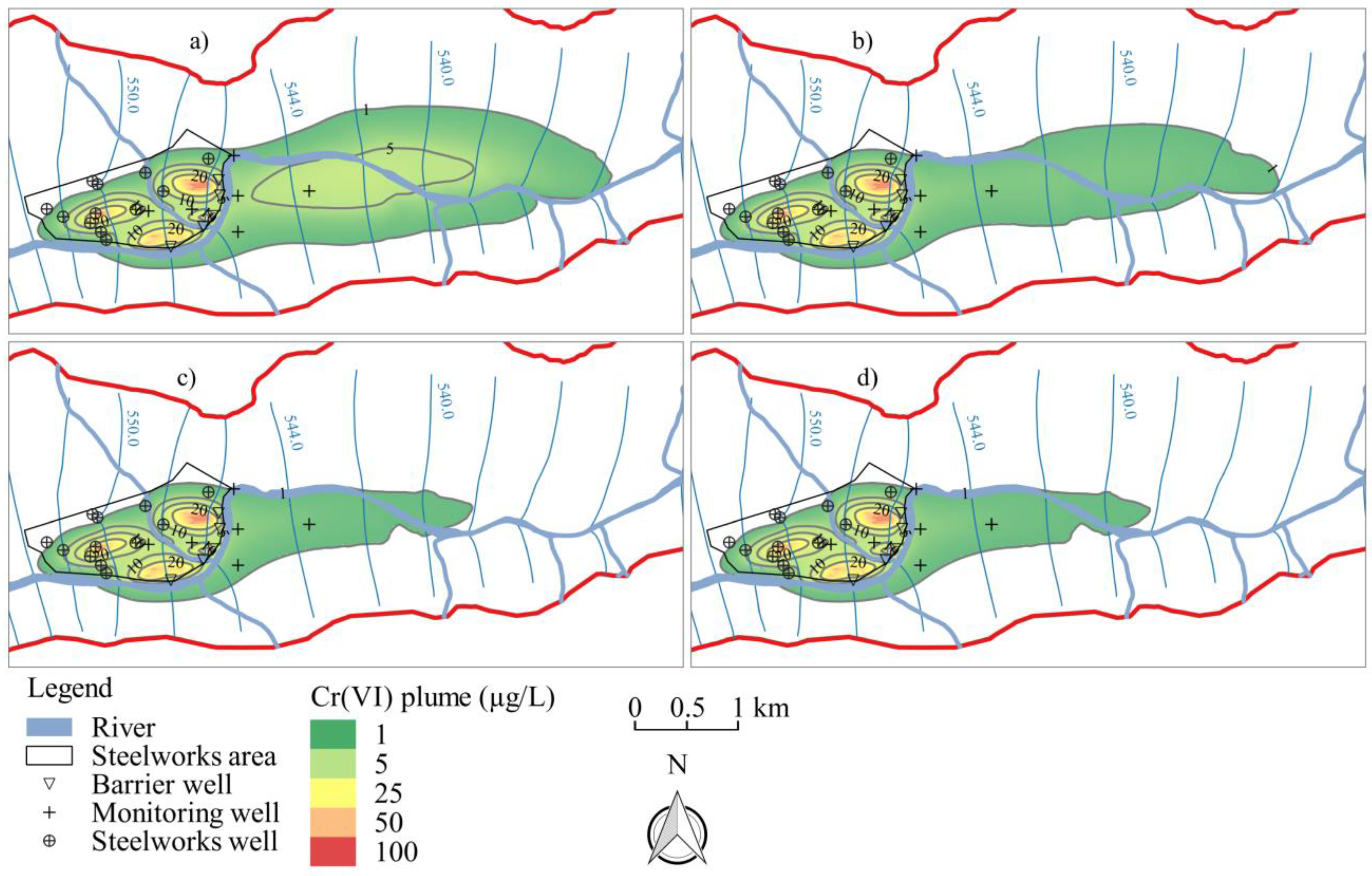
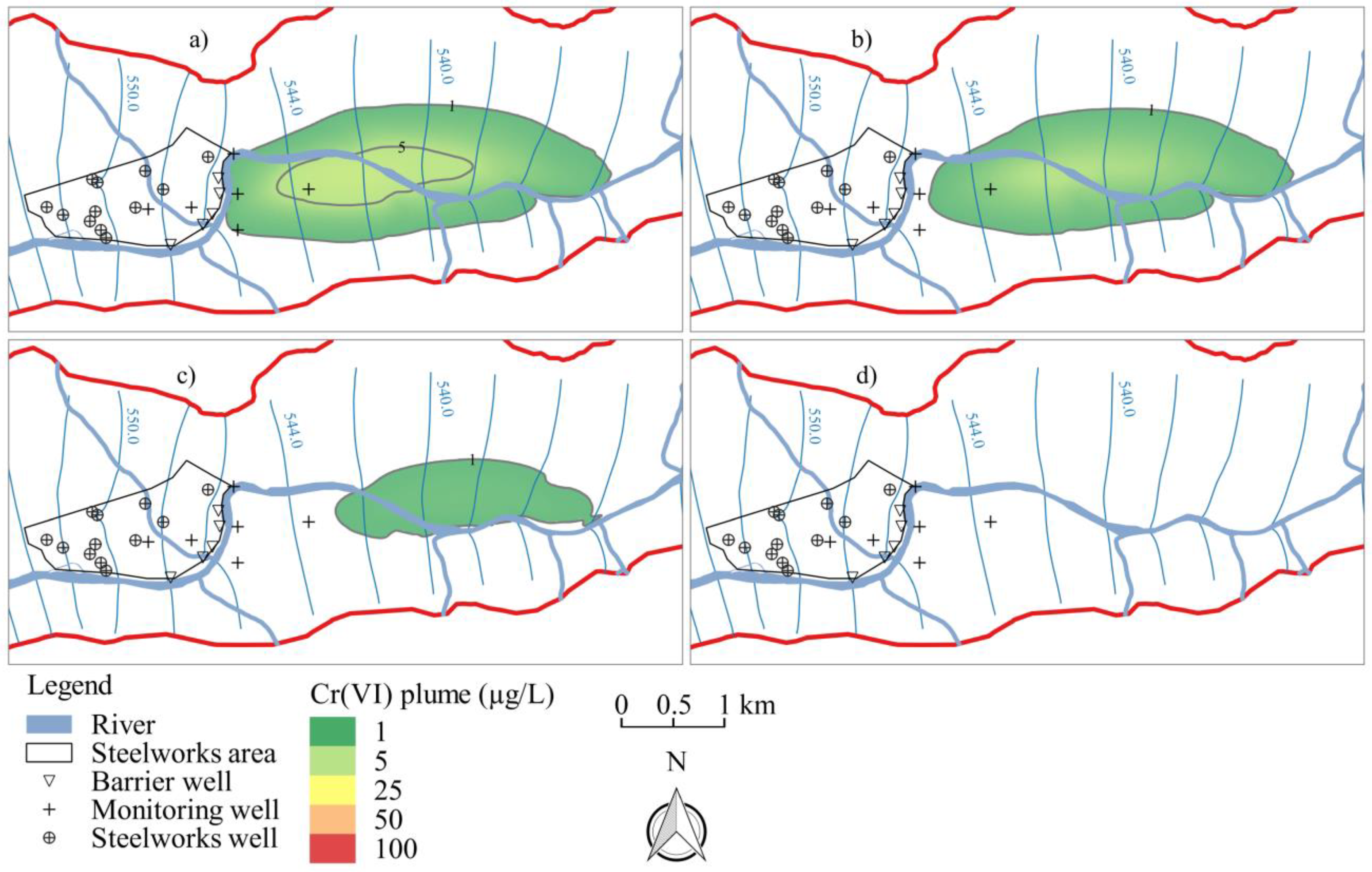
Measured concentrations of Cr(VI) in river water samples collected in February 2016 were all below the DL (i.e., <1.12 µg/L). This suggests that the Cr(VI) polluted groundwater that enters the Dora Baltea River with concentrations around 5–1 µg/L, as indicated by transport model results, are likely diluted and dispersed by the river water. The fact that no detectable Cr(VI) concentrations were found in the Dora Baltea River leads to speculate that, though the river gains Cr(VI) affected groundwater, the Cr(VI) groundwater plume has no relevant impacts on river water quality.

3.2. Scenario 1

The results for the optimal configuration of the hydraulic barrier coupled to the deactivation of some steelworks wells are:
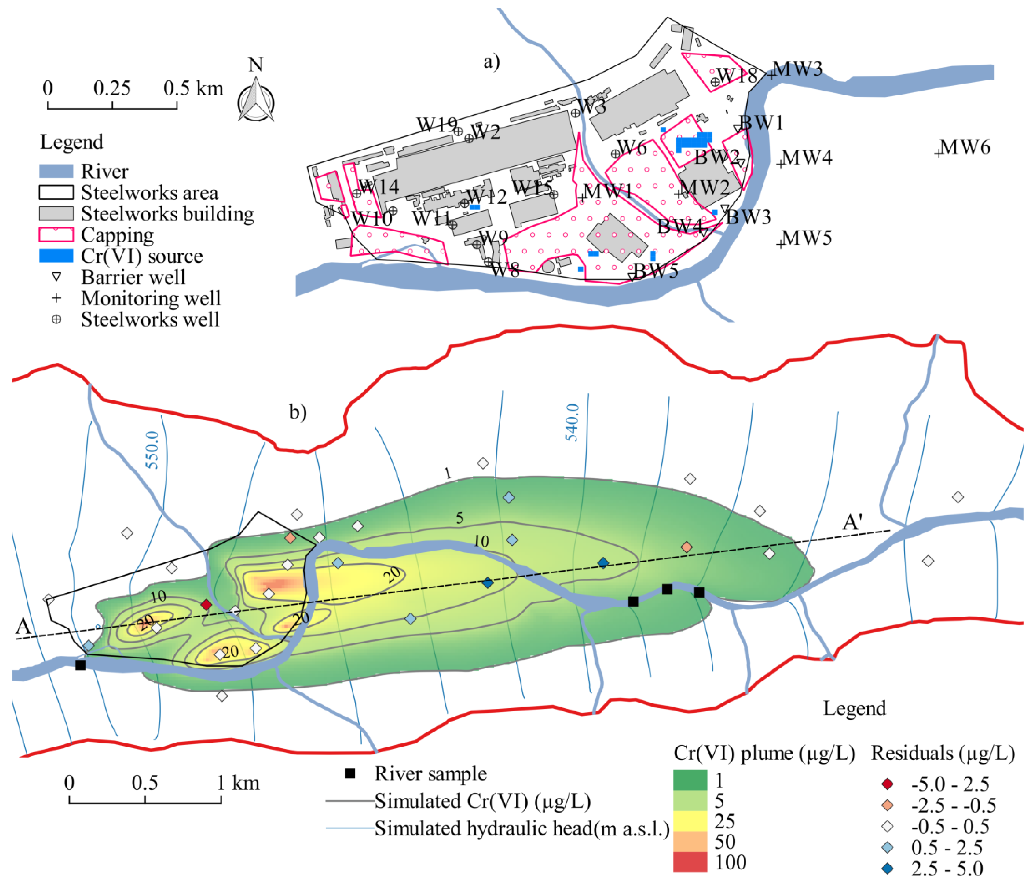
  • the hydraulic barrier is composed of 5 wells (BW) located along the eastern border of the steelworks area, their exact locations are shown in Figure 3a;
  • the depth of the hydraulic barrier wells ranges between 31 and 36 m b.g.l., the well screen interval is between model layers 3 and 6, that corresponds to ~15–20 and ~31–36 m b.g.l.;
  • the 5 hydraulic barrier wells (BW1 to BW5) have a well discharge of 6500, 7000, 7000, 6000, and 1000 m3/day, respectively, for a total discharge of 27,500 m3/day;
  • in order to compensate the discharge of the hydraulic barrier, three steelworks wells were deactivated; they are wells 6, 8, and 10 (W6, W8, and W10 in Figure 3a) with a discharge of 10,849; 862; and 13,104 m3/day, respectively (data for January 2009), that correspond to a total deactivated discharge of 24,815 m3/day;
  • in terms of well discharge, the needs of the hydraulic barrier overcome the deactivation of the steelworks wells (2685 m3/day), and this corresponds to an increase of only ~5% of the total discharge of the steelworks wells.
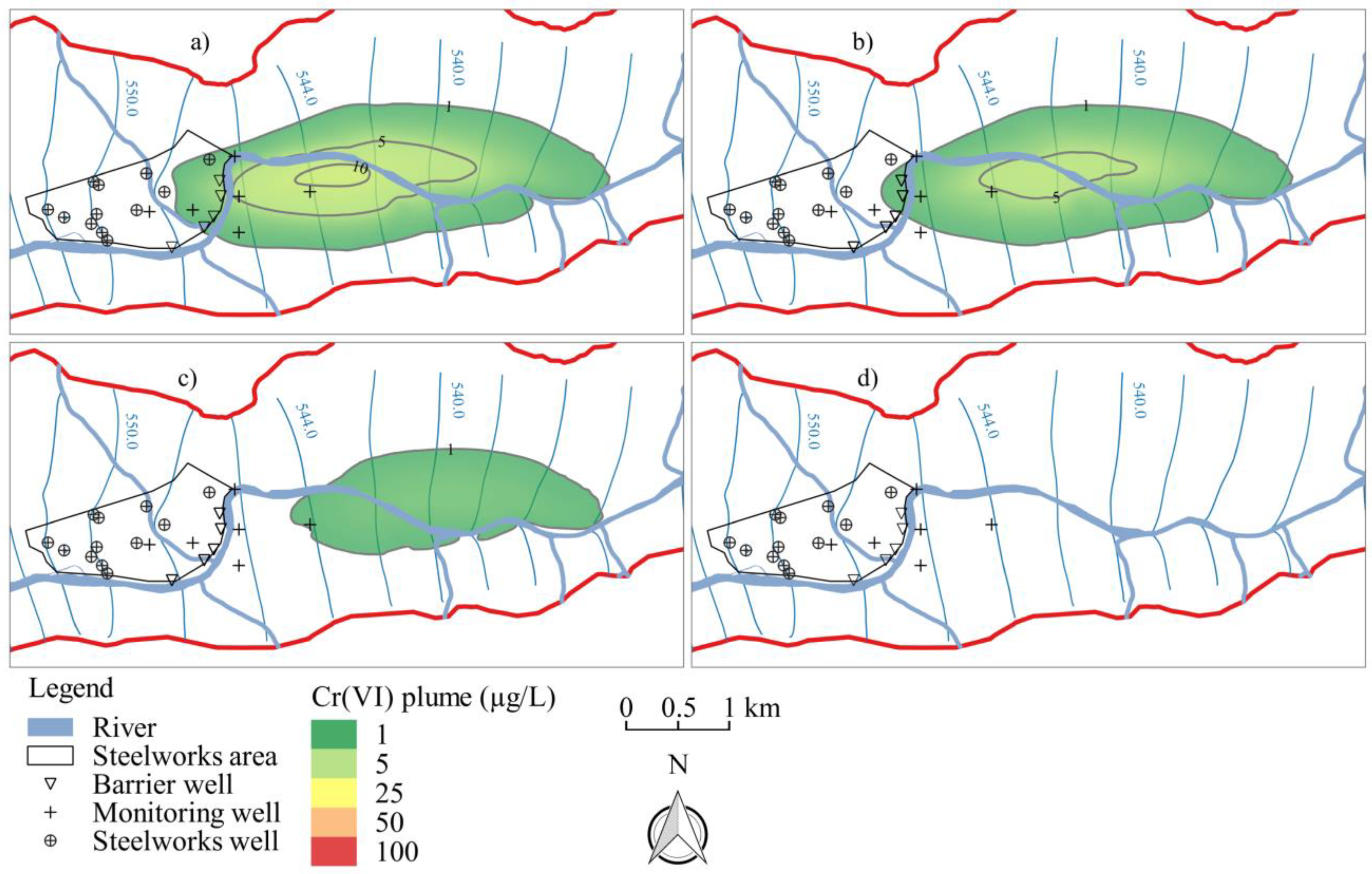
The results of the flow and transport models for Scenario 1, obtained through the optimal configuration of the hydraulic barrier described above, are shown in Figure 5. Concerning groundwater flow, the effect of the cone of depression generated by the hydraulic barrier wells can be clearly seen by the perturbation of the head contour line at 546 m a.s.l., which now crosses the steelworks area. The detailed evolution over time of the groundwater Cr(VI) concentrations during the simulation can be seen in Figure 6, which reports the breakthrough curves registered in the monitoring piezometers MW2, located ~200 m upstream of the hydraulic barrier, and MW6, located ~700 m downstream of the barrier (see Section 2.2.3 for details). These curves couple the modeled concentrations for Scenario 0 (i.e., with no hydraulic barrier; from 0 to 20 years in the graphs) with those for Scenario 1 (i.e., with the hydraulic barrier; from 20 to 40 years in the graphs). The breakthrough curve for MW2 indicates that, after the activation of the hydraulic barrier and inside the steelworks area, the Cr(VI) concentrations decrease in the shallower part of the aquifer (e.g., from ~10 to 8 µg/L in layer 3), remaining, however, above the limit of 5 µg/L, whereas in the deeper part of the aquifer, the concentrations, which are, however, below the limit of 5 µg/L, have a slight increase. The latter is likely related to the deviation of the plume towards the wells of the hydraulic barrier, so producing an increase of concentrations that is seen in the layers not tapped by the wells of the barrier (i.e., below layer 6). The breakthrough curve for MW6 shows that the Cr(VI) concentrations in all layers drop below the limit of 5 µg/L after ~3 years from the activation of the barrier (i.e., 23 years in Figure 6). The maximum concentration stands around 3 µg/L, whereas it was ~14 µg/L for Scenario 0.
Other useful information can be given by the analysis of the transport model mass balance. After 20 years of working of the hydraulic barrier, the total Cr(VI) mass in the aquifer decreases of ~46%, passing from ~140 to ~75 kg (Figure 7). This also alleviates the Cr(VI) load entering the Dora Baltea River along its gaining stretch, indeed the content of Cr(VI) gained by the river decreased by 36% with respect to Scenario 0. Conversely, the Cr(VI) mass abstracted by the wells, so including also the hydraulic barrier wells, increased by 520% with respect to Scenario 0.

3.3. Scenario 2

Figure 8 shows the results of the transport model for Scenario 2. As expected, the removal of the Cr(VI) sources leads to a more rapid and complete remediation of the groundwater plume. Figure 6 shows that, in monitoring piezometer MW2, the Cr(VI) concentrations drop below the limit of 5 µg/L after ~1 year from the removal of the sources (i.e., 21 years in Figure 6), and approach values close to zero in all layers after ~6 years (i.e., 26 years in Figure 6). The breakthrough curve for MW6 indicates that at ~700 m downstream of the steelworks area the Cr(VI) drops below 5 µg/L after ~2.5 years from the removal of the sources (i.e., 22.5 years in Figure 6), and approach values close to zero in all layers after ~10 years (i.e., 30 years in Figure 6). The Figure 7 shows that the total Cr(VI) mass in the aquifer approaches values close to zero after 17 years from the source removal. The rate of Cr(VI) attenuation is faster within the first 6 years from the removal; in this period, the Cr(VI) mass decreases of ~82%, whereas in the following 11 years the Cr(VI) decreases of only 18%.

3.4. Scenario 3

Modeled Cr(VI) concentrations for Scenario 3 are shown in Figure 9. The joint removal of the Cr(VI) sources and the activation of the hydraulic barrier lead to a faster removal of Cr(VI) from groundwater. This is especially seen within the steelworks area, where the hydraulic barrier has its capture zone. Indeed, Figure 6 shows that in monitoring piezometer MW2, located within the steelworks, the Cr(VI) concentrations approach values close to zero in all layers after only ~4 years from the starting of the remediation works (i.e., 24 years in Figure 6). Concerning the monitoring piezometer MW6, its Cr(VI) concentrations drop below 5 µg/L after ~2.3 years from the remediation works (i.e., 22.3 years in Figure 6) and approach values close to zero in all layers after ~9 years (i.e., 29 years in Figure 6). Figure 7 shows that the curve of decrease of total Cr(VI) mass in the aquifer for Scenario 3 is similar to that for Scenario 2, however, during the first 5 years after the starting of the remediation works, the decrease of Cr(VI) mass in the Scenario 3 is ~1 year faster with respect to Scenario 2. After 14 years from the starting of the remediation works, the total Cr(VI) mass in the aquifer between Scenario 2 and Scenario 3 is the same.

3.5. Advantages and Disadvantages of Modeled Scenarios

The remediation work simulated in the Scenario 1, that is the activation of the hydraulic barrier within the steelworks area, could represent an effective action that can be taken in the short term for containing the Cr(VI) pollution affecting large portions of the Aosta Plain aquifer, which is also used for drinking water purposes. The optimization of the discharge of the barrier through the deactivation of three steelworks wells has two main advantages: (a) a limited impact on groundwater resource quantity, so preventing the overexploitation of the aquifer that, in particular, should be avoided during drought periods; (b) the increase of only 5% of total groundwater abstraction by the steelworks for its industrial processes would facilitate the management of the polluted water abstracted by the hydraulic barrier. However, the adoption of the sole hydraulic barrier would only contain the Cr(VI) concentrations above 5 µg/L within the steelwork area, and would not represent a full remediation of the Cr(VI) pollution.
Conversely, the source removal considered in the Scenario 2 would be only carried out over the long term, since it requires the specific evaluation of the best remediation technique applicable to the steelworks unsaturated zone. However, the source removal would represent a full remediation work allowing for a complete cleaning up of the polluted aquifer.
Concerning the combination of the hydraulic barrier and source removal simulated in the Scenario 3, since the former only collects the Cr(VI) plume within the steelwork area, it could be deactivated after the Cr(VI) concentrations inside the steelwork approach values close to zero, a point that can be reached after 4–5 years from the activation of the remediation works, as suggested by the breakthrough curve of monitoring piezometer MW2.

4. Conclusions

This work presented a numerical 3D modeling of groundwater flow and Cr(VI) transport for simulating the adoption of some remediation works for containing and attenuating the Cr(VI) pollution which affects the Aosta Plain aquifer (N Italy). On the basis of the modeling results, the following main suggestions aimed at supporting the improvement of groundwater quality in the Aosta Plain can be done:
  • a hydraulic barrier composed of five wells located along the eastern border of the steelwork area would contain Cr(VI) concentrations above 5 µg/L (i.e., the Italian regulatory limit) within the steelwork area; these five wells, tapping the aquifer between ~15–20 and ~31–36 m b.g.l., would have a total discharge of 27,500 m3/day; this value of discharge would be compensated by the deactivation of three steelwork wells (for a total deactivated discharge of 24,815 m3/day), in order to limit the impact of the barrier on groundwater resources quantity;
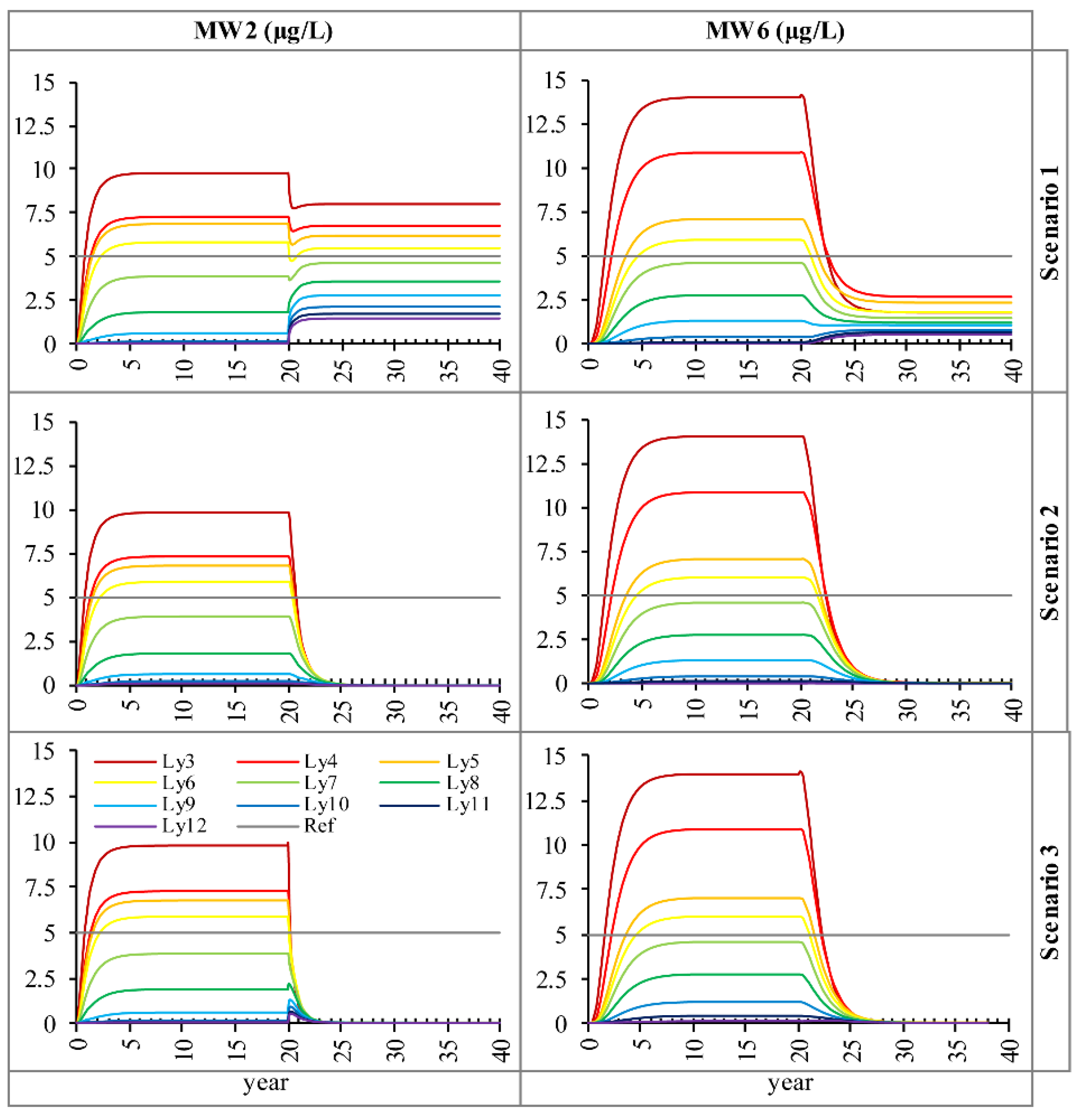
  • this hydraulic barrier would drop the Cr(VI) concentrations below 5 µg/L in the areas downstream of the steelwork after ~3 years from its start of operation;
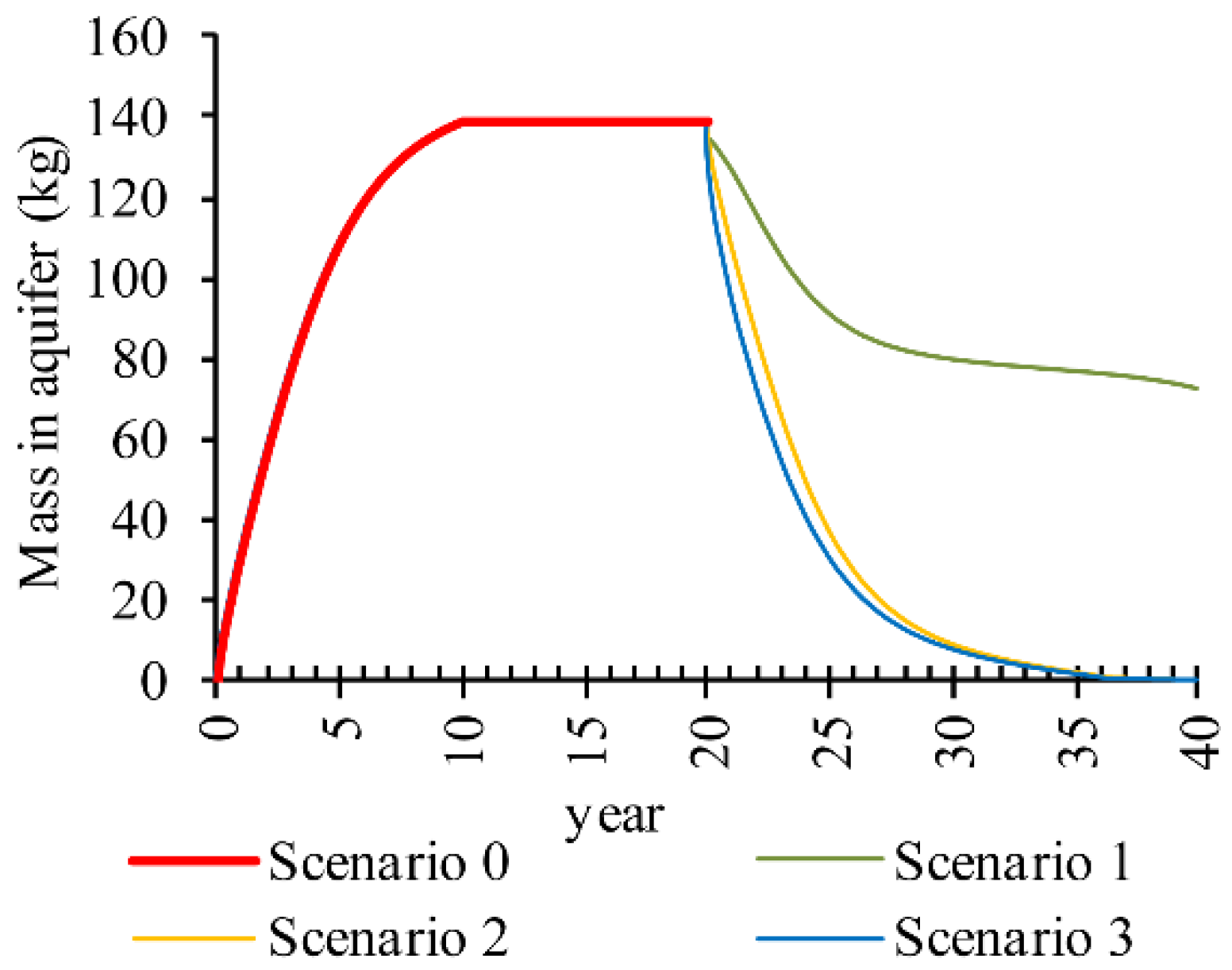
  • a remediation work aimed at removing the Cr(VI) sources from the unsaturated zone would have better results with respect to the activation of the hydraulic barrier: a full remediation of the Cr(VI) groundwater plume would be obtained after 17 years from the sources removal, with a fall of ~82% of Cr(VI) mass in aquifer within the first 6 years;
  • for a faster remediation, the removal of the Cr(VI) sources from the unsaturated zone would be accompanied by the activation of the hydraulic barrier; the working of the barrier would be needed only for the first 4–5 years.
This work represented an example of the application of flow and transport modeling to support the implementation of remediation works aimed at improving the groundwater quality, so the methodology used here could be applied in other similar case studies worldwide.
Future works involving the modeling of Cr(VI) transport in the Aosta Plain aquifers will be addressed, considering a transient transport modeling based on a transient flow model [27] and using the newest transport code MT3D-USGS [46] which supports the SFR2 package for simulating groundwater/surface water interactions.

Author Contributions

Conceptualization, G.A.S. and M.R.; Formal analysis, G.A.S.; Funding acquisition, L.F. and T.B.; Investigation, G.A.S. and C.Z.; Methodology, G.A.S., M.R., L.F. and T.B.; Project administration, L.F. and T.B.; Resources, T.B.; Supervision, M.R., L.F. and T.B.; Visualization, G.A.S.; Writing–original draft, M.R.; Writing–review & editing, G.A.S., L.F., C.Z. and T.B.

Funding

This research was funded by the Regional Environmental Protection Agency–Aosta Valley Region through the scientific collaboration number 2-18-2009100-3.

Acknowledgments

The authors are grateful to Pietro Capodaglio and Fulvio Simonetto, Regional Environmental Protection Agency–Aosta Valley Region, for supporting this study. The Gocad Research Group and Paradigm Geophysical are acknowledged for welcoming the University of Milano-Bicocca into the Gocad Consortium (http://www.ring-team.org/home).

Conflicts of Interest

The authors declare no conflict of interest.

References

  1. McDonald, M.G.; Harbaugh, A.W. A Modular Three-Dimensional Finite-Difference Ground-Water Flow Model; Techniques of Water-Resources Investigations, Book 6, Chapter A1; US Geological Survey: Reston, VA, USA, 1988.
  2. Pollock, D.W. User Guide for MODPAHT Version 6—A Particle-Tracking Model for MODFLOW; Techniques and Methods 6–A41; US Geological Survey: Reston, VA, USA, 2012; p. 58.
  3. Zheng, C.; Wang, P. MT3DMS: A Modular Three-Dimensional Multispecies Model for Simulation of Advection, Dispersion and Chemical Reactions of Contaminants in Groundwater Systems; Documentation and User’s Guide; U.S. Army Engineer Research and Development Center Contract Report SERDP-99-1; The University of Alabama: Vicksburg, MS, USA, 1999; p. 202. [Google Scholar]
  4. Guo, W.; Langevin, C.D. User’s Guide to SEAWAT: A Computer Program for Simulation of Three-Dimensional Variable-Density Ground-Water Flow; Techniques of Water-Resources Investigations 6-A7; US Geological Survey: Reston, VA, USA, 2002; p. 77.
  5. Alberti, L.; Colombo, L.; Formentin, G. Null-space Monte Carlo particle tracking to assess groundwater PCE (Tetrachloroethene) diffuse pollution in north-eastern Milan functional urban area. Sci. Total Environ. 2018, 621, 326–339. [Google Scholar] [CrossRef] [PubMed]
  6. Chelli, A.; Zanini, A.; Petrella, E.; Feo, A.; Celico, F. A multidisciplinary procedure to evaluate and optimize the efficacy of hydraulic barriers in contaminated sites: A case study in Northern Italy. Environ. Earth Sci. 2018, 77, 246. [Google Scholar] [CrossRef]
  7. Colombani, N.; Mastrocicco, M.; Prommer, H.; Sbarbati, C.; Petitta, M. Fate of arsenic, phosphate and ammonium plumes in a coastal aquifer affected by saltwater intrusion. J. Contam. Hydrol. 2015, 179, 116–131. [Google Scholar] [CrossRef] [PubMed]
  8. Colombani, N.; Osti, A.; Volta, G.; Mastrocicco, M. Impact of climate change on salinization of coastal water resources. Water Resour. Manag. 2016, 30, 2483–2496. [Google Scholar] [CrossRef]
  9. Grava, A.; Rotiroti, M.; Fumagalli, L.; Bonomi, T. Optimization of a well system using the ground water management package of MODFLOW-2000. Rend. Online Soc. Geol. Ital. 2016, 39, 101–104. [Google Scholar] [CrossRef]
  10. Post, V.E.A.; Houben, G.J. Density-driven vertical transport of saltwater through the freshwater lens on the island of Baltrum (Germany) following the 1962 storm flood. J. Hydrol. 2017, 551, 689–702. [Google Scholar] [CrossRef]
  11. Dokou, Z.; Karagiorgi, V.; Karatzas, G.P.; Nikolaidis, N.P.; Kalogerakis, N. Large scale groundwater flow and hexavalent chromium transport modeling under current and future climatic conditions: The case of Asopos River Basin. Environ. Sci. Pollut. Res. 2016, 23, 5307–5321. [Google Scholar] [CrossRef] [PubMed]
  12. Dokou, Z.; Karatzas, G.P.; Panagiotakis, I.; Dermatas, D. Groundwater modeling and remediation scenarios of a hexavalent chromium plume released from an industrial site. Bull. Environ. Contam. Toxicol. 2017, 98, 338–346. [Google Scholar] [CrossRef] [PubMed]
  13. Friedly, J.C.; Davis, J.A.; Kent, D.B. Modeling hexavalent chromium reduction in groundwater in field-scale transport and laboratory batch experiments. Water Resour. Res. 1995, 31, 2783–2794. [Google Scholar] [CrossRef]
  14. Mayer, K.U.; Blowes, D.W.; Frind, E.O. Reactive transport modeling of an in situ reactive barrier for the treatment of hexavalent chromium and trichloroethylene in groundwater. Water Resour. Res. 2001, 37, 3091–3103. [Google Scholar] [CrossRef] [Green Version]
  15. Rivero, M.J.; Primo, O.; Ortiz, M.I. Modelling of Cr(VI) removal from polluted groundwaters by ion exchange. J. Chem. Technol. Biotechnol. 2004, 79, 822–829. [Google Scholar] [CrossRef]
  16. Thacher, R.; Hsu, L.; Ravindran, V.; Nealson, K.H.; Pirbazari, M. Modeling the transport and bioreduction of hexavalent chromium in aquifers: Influence of natural organic matter. Chem. Eng. Sci. 2015, 138, 552–565. [Google Scholar] [CrossRef]
  17. Tiwary, R.K.; Dhakate, R.; Ananda Rao, V.; Singh, V.S. Assessment and prediction of contaminant migration in ground water from chromite waste dump. Environ. Geol. 2005, 48, 420–429. [Google Scholar] [CrossRef]
  18. Wanner, C.; Eggenberger, U.; Mäder, U. Reactive transport modelling of Cr(VI) treatment by cast iron under fast flow conditions. Appl. Geochem. 2011, 26, 1513–1523. [Google Scholar] [CrossRef]
  19. Wanner, C.; Zink, S.; Eggenberger, U.; Mäder, U. Assessing the Cr(VI) reduction efficiency of a permeable reactive barrier using Cr isotope measurements and 2D reactive transport modeling. J. Contam. Hydrol. 2012, 131, 54–63. [Google Scholar] [CrossRef] [PubMed]
  20. Tiwari, A.K.; De Maio, M. Assessment of risk to human health due to intake of chromium in the groundwater of the Aosta Valley region, Italy. Hum. Ecol. Risk Assess. 2017, 23, 1153–1163. [Google Scholar] [CrossRef]
  21. Bonomi, T.; Fumagalli, L.; Stefania, G.A.; Rotiroti, M.; Pellicioli, F.; Simonetto, F.; Capodaglio, P. Groundwater contamination by Cr(VI) in the Aosta Plain (Northern Italy): Characterization and preliminary modeling. Rend. Online Soc. Geol. Ital. 2015, 35, 21–24. [Google Scholar] [CrossRef]
  22. Bonomi, T.; Fumagalli, M.; Benastini, V.; Rotiroti, M.; Capodaglio, P.; Simonetto, F. Preliminary groundwater modelling by considering the interaction with superficial water: Aosta Plain case (Northern Italy). Acque Sotter. Ital. J. Groundw. 2013, 2, 31–45. [Google Scholar] [CrossRef]
  23. Bonomi, T.; Fumagalli, M.; Rotiroti, M.; Perego, R.; Simonetto, F.; Capodaglio, P. Groundwater flow modelling of the Aosta Plain in northern Italy. In Engineering Geology for Society and Territory; Lollino, G., Arattano, M., Rinaldi, M., Giustolisi, O., Marechal, J.-C., Grant, G.E., Eds.; Springer: Berlin/Heidelberg, Germany, 2015; pp. 227–230. [Google Scholar]
  24. Novel, J.P.; Puig, J.M.; Zuppi, G.M.; Dray, M.; Dzikowski, M.; Jusserand, C.; Money, E.; Nicoud, G.; Parriaux, A.; Pollicini, F. Complexité des circulations dans l’aquifère alluvial de la plaine d’Aoste (Italie): Mise en évidence par l’hydrogéochimie. Eclogae Geol. Helv. 2002, 95, 323–331. [Google Scholar]
  25. Rotiroti, M.; Di Mauro, B.; Fumagalli, L.; Bonomi, T. COMPSEC, a new tool to derive natural background levels by the component separation approach: Application in two different hydrogeological contexts in northern Italy. J. Geochem. Explor. 2015, 158, 44–54. [Google Scholar] [CrossRef]
  26. Rotiroti, M.; Fumagalli, L.; Frigerio, M.C.; Stefania, G.A.; Simonetto, F.; Capodaglio, P.; Bonomi, T. Natural background levels and threshold values of selected species in the alluvial aquifers in the Aosta Valley Region (N Italy). Rend. Online Soc. Geol. Ital. 2015, 35, 256–259. [Google Scholar] [CrossRef]
  27. Stefania, G.A.; Rotiroti, M.; Fumagalli, L.; Simonetto, F.; Capodaglio, P.; Zanotti, C.; Bonomi, T. Modeling groundwater/surface-water interactions in an Alpine valley (the Aosta Plain, NW Italy): The effect of groundwater abstraction on surface-water resources. Hydrogeol. J. 2018, 26, 147–162. [Google Scholar] [CrossRef]
  28. Tiwari, A.K.; De Maio, M.; Amanzio, G. Evaluation of metal contamination in the groundwater of the Aosta Valley region, Italy. Int. J. Environ. Res. 2017, 11, 291–300. [Google Scholar] [CrossRef]
  29. Tiwari, A.K.; Nota, N.; Marchionatti, F.; De Maio, M. Groundwater-level risk assessment by using statistical and geographic information system (GIS) techniques: A case study in the Aosta Valley region, Italy. Geomat. Nat. Hazards Risk 2017, 8, 1396–1406. [Google Scholar] [CrossRef]
  30. Triganon, A.; Dzikowski, M.; Novel, J.P.; Dray, M.; Zuppi, G.M.; Parriaux, A. Échanges nappe–rivière en vallée alpine: Quantification et modélisation (Vallée d’Aoste, Italie). Can. J. Earth Sci. 2003, 40, 775–786. [Google Scholar] [CrossRef]
  31. European Commission. Directive 2000/60/EC of the European Parliament and of the Council of 23 October 2000 establishing the framework of Community action in the field of water policy. Off. J. Eur. Commun. 2000, 43, L327/1. [Google Scholar]
  32. Rotiroti, M.; Fumagalli, L.; Stefania, G.A.; Frigerio, M.C.; Simonetto, F.; Capodaglio, P.; Bonomi, T. Assessment of the chemical status of the alluvial aquifer in the Aosta Plain: An example of the implementation of the Water Framework Directive in Italy. Geophys. Res. Abstr. 2015, 17, 4044. [Google Scholar]
  33. Harbaugh, A.W.; Banta, E.R.; Hill, M.C.; McDonald, M.G. MODFLOW-2000, the U.S. Geological Survey Modular Ground-Water Model—User Guide to Modularization Concepts and the Ground-Water Flow Process; Open-File Report 00-92; US Geological Survey: Reston, VA, USA, 2000; p. 121.
  34. Bonomi, T.; Fumagalli, M.; Rotiroti, M.; Bellani, A.; Cavallin, A. The hydrogeological well database TANGRAM©: A tool for data processing to support groundwater assessment. Acque Sotter. Ital. J. Groundw. 2014, 3, 35–45. [Google Scholar] [CrossRef]
  35. Bonomi, T. Database development and 3D modeling of textural variations in heterogeneous, unconsolidated aquifer media: Application to the Milan plain. Comput. Geosci. 2009, 35, 134–145. [Google Scholar] [CrossRef]
  36. Fabbri, P.; Trevisani, S. A geostatistical simulation approach to a pollution case in northeastern Italy. Math. Geol. 2005, 37, 569–586. [Google Scholar] [CrossRef]
  37. Perego, R.; Bonomi, T.; Fumagalli, L.; Benastini, V.; Aghib, F.; Rotiroti, M.; Cavallin, A. 3D reconstruction of the multi-layer aquifer in a Po Plain area. Rend. Online Soc. Geol. Ital. 2014, 30, 41–44. [Google Scholar] [CrossRef]
  38. Rotiroti, M.; Jakobsen, R.; Fumagalli, L.; Bonomi, T. Arsenic release and attenuation in a multilayer aquifer in the Po Plain (Northern Italy): Reactive transport modeling. Appl. Geochem. 2015, 63, 599–609. [Google Scholar] [CrossRef]
  39. Pollicini, F. Geologia ed Idrogeologia Della Piana di Aosta. Master’s Thesis, University of Turin, Turin, Italy, 1994. [Google Scholar]
  40. De Luca, D.; Masciocco, L.; Motta, E.V.; Tonussi, M. Studio Geologico Finalizzato Alla Definizione Delle Aree di Salvaguardia Dei Pozzi di Acquedotto Del Comune di AOSTA; University of Turin: Turin, Italy, 2004. [Google Scholar]
  41. Niswonger, R.G.; Prudic, D.E. Documentation of the Streamflow-Routing (SFR2) Package to Include Unsaturated Flow Beneath Streams: A Modification to SFR1; Techniques and Methods 6-A13; US Geological Survey: Reston, VA, USA, 2005; p. 50.
  42. Mercado, A. The spreading pattern of injected water in a permeability stratified aquifer. Int. Assoc. Hydrol. Sci. 1967, 72, 23–36. [Google Scholar]
  43. Gazzetta Ufficiale. Decreto Legislativo 3 aprile 2006, n. 152. In Norme in Materia Ambientale; Gazzetta Ufficiale: Rome, Italy, 2006. [Google Scholar]
  44. Xu, Y.; Zhao, D. Reductive immobilization of chromate in water and soil using stabilized iron nanoparticles. Water Res. 2007, 41, 2101–2108. [Google Scholar] [CrossRef] [PubMed]
  45. Anjana, K.; Kaushik, A.; Kiran, B.; Nisha, R. Biosorption of Cr(VI) by immobilized biomass of two indigenous strains of cyanobacteria isolated from metal contaminated soil. J. Hazards Mater. 2007, 148, 383–386. [Google Scholar] [CrossRef] [PubMed]
  46. Bedekar, V.; Morway, E.D.; Langevin, C.D.; Tonkin, M.J. MT3D-USGS Version 1: A U.S. Geological Survey Release of MT3DMS Updated with New and Expanded Transport Capabilities for Use with MODFLOW; Techniques and Methods 6-A53; US Geological Survey: Reston, VA, USA, 2016; p. 84.
Figure 1. (a) Study area with hydrography and hydraulic head contour lines resulted from the flow model and location of the cross-section (1-1′) of Figure 2 and the lithologs used for the 3D reconstruction of hydraulic conductivity. (b) Maximum concentrations of Cr(VI) measured in the period 2003–2011. (c) Localization of the study area.
Geosciences 08 00209 g001
Figure 2. Lithological cross-section of the study area schematizing the aquifer structure.
Geosciences 08 00209 g002
Figure 3. (a) The steelworks area with location of steelwork wells (Wn), hydraulic barrier wells (BWn), monitoring piezometers (MWn), and Cr(VI) source areas. (b) Modeled hydraulic heads and Cr(VI) concentrations for Scenario 0 after 20 years of simulation within model layer 3, with location of transport calibration targets (with respective residual values), river water sampling points and location of the cross-section (A–A’) of Figure 4.
Geosciences 08 00209 g003
Figure 4. Modeled Cr(VI) concentrations for Scenario 0 after 20 years of simulation along the cross-section A–A’ (see Figure 3 for location).
Geosciences 08 00209 g004
Figure 5. Modeled hydraulic heads and Cr(VI) concentrations for Scenario 1 within model layer 3 after 2 (a), 5 (b), 10 (c), and 20 (d) years of simulation.
Geosciences 08 00209 g005
Figure 6. Breakthrough curve of modeled Cr(VI) concentrations (µg/L) for monitoring piezometers MW2 and MW6 (locations are displayed in Figure 3a); concentrations from 0 to 20 years are the results for Scenario 0, whereas from 20 to 40 years, the results of the three scenarios are displayed: Scenario 1 (activation of a hydraulic barrier), Scenario 2 (natural attenuation after the complete removal of the Cr(VI) source), Scenario 3 (combination of the previous two works). Ly: model layer; ref: the Italian regulatory limit for Cr(VI).
Geosciences 08 00209 g006
Figure 7. Total modeled Cr(VI) mass in aquifer over simulation time for the different considered scenarios.
Geosciences 08 00209 g007
Figure 8. Modeled Cr(VI) concentrations for Scenario 2 within model layer 3 after 2 (a), 3 (b), 5 (c), and 7 (d) years of simulation; hydraulic heads are the same as for Scenario 0.
Geosciences 08 00209 g008
Figure 9. Modeled hydraulic heads and Cr(VI) concentrations for Scenario 3 within model layer 3 after 2 (a), 3 (b), 5 (c), and 7 (d) years of simulation.
Geosciences 08 00209 g009

