Reactive and Mixing Processes Governing Ammonium and Nitrate Coexistence in a Polluted Coastal Aquifer

Abstract

A comprehensive hydrochemical, stable isotope and microbial analyses characterisation has been performed to evaluate the sources of groundwater, nitrogen pollution and degradation processes occurring in an industrial polluted coastal aquifer in the framework of a complex hydrodynamic system. The coexistence of ammonium and nitrate has been observed in almost all the investigated monitoring wells, reaching maximum values of 100 and 200 mg/L for both species. Chloride and potassium concentration coupled with groundwater stable isotopes data show the influence of local and urban recharge and the occurrence of seawater intrusion in areas near the coastline. δ¹⁵N–NH₄⁺ values ranging between −4.9 and +14.9% suggest that different processes such as partial nitrification of ammonium, probably anammox activities and sorption, are occurring at the site. The isotope data for NH₄⁺ also showed the existence of the remnant of an old fertilizer plume in the downgradient area. The nitrate isotope data ranging between +9 and +46% and +6 and +26% for δ¹⁵N–NO₃⁻ and δ¹⁸O–NO₃⁻, respectively, suggest that nitrate content is attenuated by denitrification and probably annamox. The fast groundwater flow field is one of the reasons for the coexistence of NH₄⁺ and NO₃⁻ in groundwater, since both compounds can penetrate the reducing zone of the aquifer. The influence of leakage of sewage pipelines on the aquifer cannot be discerned due to the complexities of the nitrogen attenuation processes, also influenced by pumping activities.

1. Introduction

Nitrate (NO₃⁻) and ammonium (NH₄⁺) are often recognised as major contaminants in both surface water and groundwater [1,2,3]. The causes can be multiple, including fertilizers leaching in agricultural environments [4,5,6,7], storm and sewage water spillages in urban environments [8,9,10], natural elevated background concentrations [11,12] and spillages of complex chemical mixtures below industrial plants [13,14]. Moreover, the nitrification of NH₄⁺ into NO₃⁻ in oxic environments often leads to an increased NO₃⁻ concentration along the flow paths, up to values well beyond to the maximum water quality admissible levels [15]. Accordingly, the origin and transformation of NH4+ in groundwater is a key issue in water quality assessments. The nitrification process is kinetically driven and depends on many factors, such as the availability of both electron donors and acceptors, salinity, pH and Eh [16]. Such peculiarities are exacerbated in aquifers, where partial/incomplete mixing between reactants often leads to a slowdown of the overall reaction kinetics [17] with respect to well-mixed bioreactors [18]. Indeed, partial/incomplete mixing can lead to the coexistence of thermodynamically unstable redox couples like NH₄⁺ and NO₃⁻, especially in industrial areas where both these reactive nitrogen species have been or are still used and thus various pollution sources can be active at the same site [13,19]. Such a coexistence can trigger or slow down nitrogen transformation processes like nitrification or denitrification, and the degree of partial/incomplete mixing could vary in different parts of the site, for example when “pump and treat” remediation schemes are active. Thus, it is important to understand the processes that induce NH₄⁺ and NO₃⁻ coexistence or the prevalence of one species over another. In addition, it is worth mentioning that NO₂⁻, an intermediate product of nitrification and denitrification, is present at a very small concentration in groundwater compared to nitrate and ammonium [20]. In recent years, nitrogen-stable isotopes are more often employed to assess different sources of pollution and nitrogen transformation in aquifers [21,22,23,24,25,26]. Although, in the abovementioned studies, NO₃⁻ was found to be the dominant nitrogen species in the oxic zone while NH₄⁺ was the dominant nitrogen species in the anoxic zone, their coexistence has been often limited to narrow reactive fringes. However, few studies have been done on the mechanisms that control NH₄⁺ and NO₃⁻ coexistence in large portions of the aquifer at the site scale [13,27].

This study aims to contribute to the understanding of nitrogen processes at industrial sites affected by different sources of nitrogen pollutants. The site under investigation is a coastal aquifer having an active hydraulic barrier designed to control the extent of contaminants plumes [19,28,29]. The approach included an evaluation of sources, distribution and degradation processes concerning reactive nitrogen species in the framework of a complex hydrodynamic system. The research tools include major ions and environmental isotopes that have been used to evaluate sources of groundwater and the sources and fate of nitrogen species. Those data have been coupled with total coliforms analysis, useful to evaluate the role of sewage leakage. The novelty of this study is to present a set of bio-geochemical analyses that provide information about the pollution sources of NH₄⁺ and NO₃⁻ and to constrain their major biogeochemical reactions in a coastal aquifer.

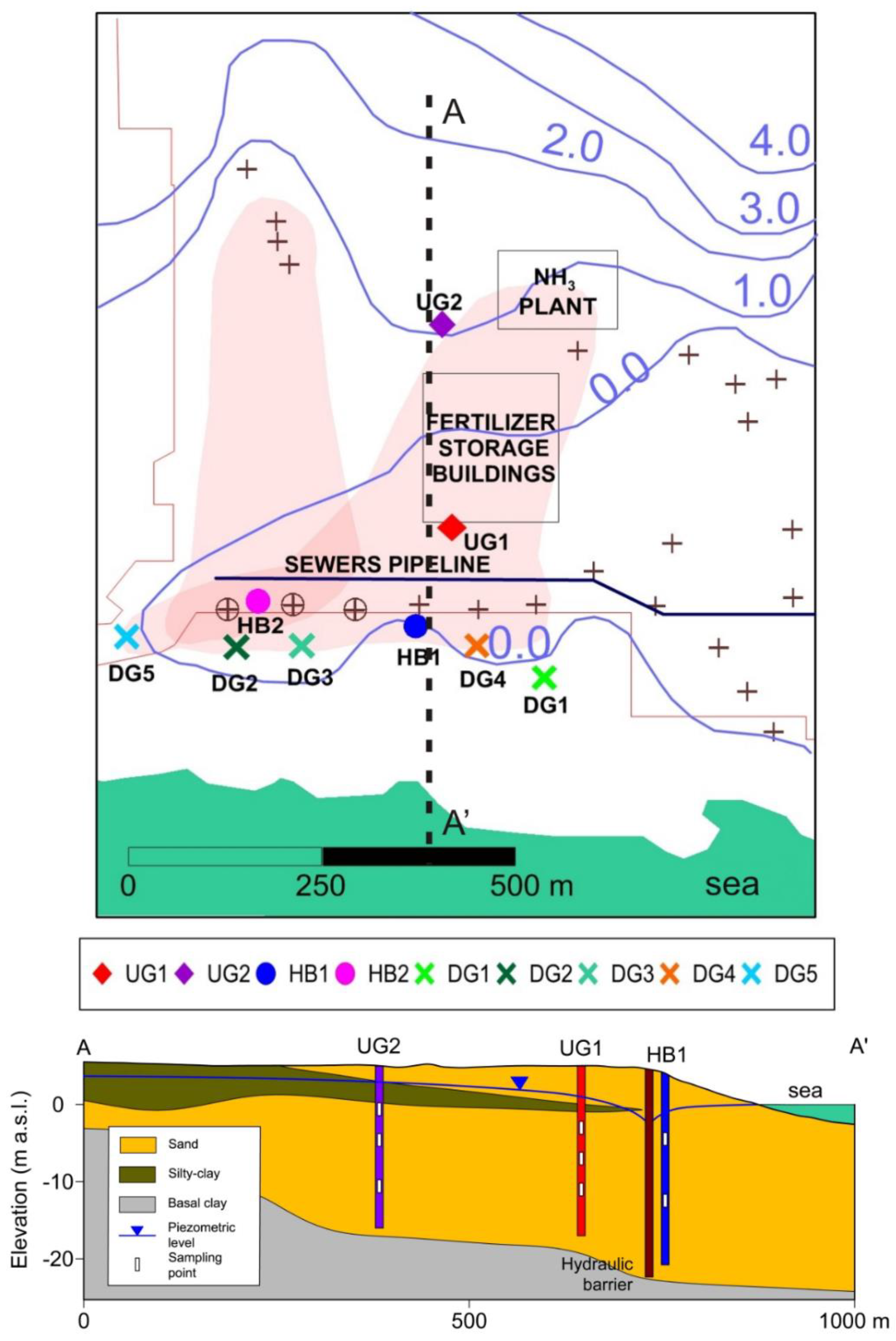
2. Geological and Hydrogeological Setting

The geological and hydrogeological setting of a portion of an industrial site is the framework for the nitrogen investigation (Figure 1). The different nitrogen pollution sources, which include a fertilizer plant, an ammonia (NH₃) production plant, and a sewage line, are also identified in Figure 1. Briefly, the unconfined aquifer is highly polluted by a range of organic and inorganic contaminants [14,19,28]. In this portion of the site, NH₄⁺ and NO₃⁻ exhibited historical concentrations up to 3000 and 500 mg/L, respectively. The unconfined aquifer is formed by fine to coarse Quaternary sandy sediments, interbedded by silty clay lenses. The aquifer is characterised by a groundwater flow system influenced by regional and local recharge and also by seawater intrusion and leakage from a sewer pipeline near the coastline. The natural groundwater flow is perpendicular to the coastline, with an average hydraulic gradient of 0.6%. A complete description of the industrial site and its hydrogeological modelling and pollutants characterisation can be found elsewhere [19,28,29]. The presence of a “pump and treat” remediation system close to the shoreline, here called for simplicity the “hydraulic barrier,” highly affects the groundwater flow system, creating large capture zones and increasing the saltwater encroachment [14]. The pumping rate of the hydraulic barrier in this area is approximately 27 L/s and the hydraulic gradient reaches a maximum of 1%. Due to the site complexity, elevated salinity, and chemical gradients present in the unconfined aquifer, a detailed vertical characterisation of the aquifer via multi-level sampling (MLS) devices was also carried out to avoid cross-contamination and misleading results.

The investigated monitoring wells have been classified, for simplicity, into three zones: MLS located upgradient (UG) with respect to the hydraulic barrier, near (HB) the hydraulic barrier, and downgradient (DG) with respect to the hydraulic barrier. This configuration allows us to identify the location and the composition of the sources of pollutants that affect the aquifer.

3. Materials and Methods

3.1. Groundwater Sampling Technique and Chemical Analysis

Groundwater has been pumped to obtain depth–discrete samples, mimicking an MLS system, from standard fully-screened monitoring wells equipped with straddle inflatable packers (800-l Solinst) to obtain ion concentrations and nitrogen isotopes depth profiles. Samples were collected in November 2011 and April 2012, during groundwater sampling surveys. The packers’ assemblage consisted of a 30 cm long sampling port, set in the middle of two inflatable packers, and a submersible centrifuge pump used for low flow purging. From each monitoring well, three to five samples have been collected at different depths, as described in Mastrocicco et al. [29] and Sbarbati et al. [19]. Samples were filtered through a 0.45 μm filter, stored in a cool box at 4 °C, and immediately transported in the laboratory. Groundwater samples collected for ion analyses have been analysed for the major ions (Cl^-, K⁺, NH₄⁺, NO₃⁻, NO₂⁻) using an isocratic dual pump ion chromatography ICS-2000 Dionex. The uncertainty of concentration results is generally lower than the detection limits. A flow-through cell has been employed to measure the in situ physical–chemical parameters (pH, electrical conductivity, Eh, dissolved oxygen) for each sampling depth, connected with a multi-parameter probe WTW Multi 340i (Weilheim, Germany), which includes: a SentiTix 41 pH combined electrode with a built-in temperature sensor for pH measurement, a combined AgCl–Pt electrode for Eh measurement and a Tetracon 325 4-electrode conductivity cell for EC measurements

3.2. Groundwater Isotopes Analyses

The stable isotope analyses in water samples (δ¹⁸O and δ²H) have been performed in the Isotopes Laboratory of the University of Parma. The oxygen isotopic composition has been measured by the water–CO₂ equilibration technique suggested by Epstein and Mayeda [30], either by manual preparation of the samples or using the Finnigan GLF 1086 (Burgwedel, Germany) automatic equilibration device [31]. The hydrogen measurements have been carried out by reducing the water sample to hydrogen by passage over hot zinc at about 520 °C according to the procedure described by Coleman et al. [32]. The isotopic measurements have been carried out using the Finnigan Delta S, Fisons Optima and Finnigan Delta Plus mass spectrometers. The isotopic results obtained are reported in terms of δ units (% deviation of the isotope ratio from the international standard VSMOW, which is 0.0); the analytical error was ±0.1% and ±1.0%, respectively for δ¹⁸O and δ²H [31].

3.3. Nitrogen Isotope Analyses

Nitrogen isotope analyses have been performed in the Environmental Isotope Laboratory of the University of Waterloo and in the Isotope Science Laboratory of the University of Calgary for NO₃⁻ isotope samples with relatively high salinity (more than 300 mg/L of Cl⁻).

Concerning δ¹⁵N–NH₄⁺ determination, a modified version of the acidified disk diffusion method [33,34] was adopted. Samples were placed in a 60 mL jar with 4 M (molar) solution of KCl (potassium chloride) and a phenolthalein indicator was added. Samples were basified with NaOH (sodium hydroxide) until the solution turned bright pink. A buffer solution of sodium tetraBorate was added and a Teflon packet containing an acidified quartz disc was added and sealed in the jar. After a period of 10 days all the ammonium in the sample should have volatilized into ammonia and been absorbed onto the acidified quartz disc as the Teflon is permeable to gas. Three internal ¹⁵NH₄⁺ isotope standards (δ¹⁵N = +0.6%, +20.9%, +35.2%) were included in each diffusion run. All standards and samples have been run in duplicate or triplicate. Once diffusion was complete, the acidified disks were frozen and freeze-dried overnight and then stored in air-tight vials. The N isotopic composition of the diffusion disks containing the NH₄⁺ as (NH₄)₂SO₄ have been analysed using a Carlo Erba 1108 Elemental Analyser interfaced with a Delta plus–IRMS (Thermo Fisher Scientific, Milan, Italy). NH₄⁺–N isotope ratios are reported in delta (δ) notation relative to atmospheric N₂. The uncertainty associated with the δ¹⁵N–NH₄⁺ analysis was generally lower than ±0.3%. As mentioned above, the analyses for δ¹⁵N–NO₃⁻ and δ¹⁸O–NO₃⁻ have been performed in two different laboratories. Groundwater samples were frozen until arrival at laboratories and analysed approximately 20 days after their collection. The samples having relative low salinity were analysed using the silver nitrate (AgNO₃) method [34] adopted in the Environmental Isotope Laboratory of the University of Waterloo. Extraction of NO₃ was performed by passing samples through an ion exchange column, followed by HCl desorption and further precipitation of AgNO₃ by the addition of Ag₂O. The obtained AgNO₃ solution was filtered in two steps at 11 and 0.45 µm to remove the precipitated AgCl and then freeze-dried to obtain solid AgNO₃. Nitrogen gas for ¹⁵N analysis was produced by combustion in the presence of CuO, Cu, and CaO. For ¹⁸O analysis, nitrate oxygen was converted to CO₂ by combusting AgNO₃ with excess graphite. ¹⁵N and ¹⁸O were analysed in a VG Micromass spectrometer and in a VG Prism Micromass spectrometer respectively. The denitrifier method” [35,36,37,38] was used at the Isotope Science Laboratory of Calgary University for high-salinity samples; the method is based on the bacterial reduction of nitrate (NO₃⁻) to nitrous oxide (N₂O) via a bacterium that lacks nitrous oxide reductase, so further reduction to N₂ does not occur. This enables simultaneous determination of both δ¹⁵N and δ¹⁸O values of the sample NO₃⁻ by measuring the δ¹⁵N and δ¹⁸O values of the produced N₂O. The bacterial strain Pseudomonas aureofaciens is used to reduce NO₃⁻ to N₂O. The system is comprised of a home-made, 24-vial auto-sampler interfaced to a HP 6890 gas chromatogram with a PreCon^® device (Wilmington, DE, USA) interfaced to a Finnigan Mat Delta + XL mass spectrometer. The accuracy and precision of δ¹⁵N and δ¹⁸O determinations based on a long-term record of analyses of ISL in-house reference (ISL-KNO3) are 0.3% and 0.7%, respectively.

3.4. Total Coliform Analysis

For total coliform analysis, groundwater samples were collected directly from pumping and monitoring wells in duplicate sterile 100-mL bottles containing sodium thiosulfate and stored at 4 °C in the dark until incubation for measuring the total coliforms. Samples were analysed for total coliforms in the laboratory of the Department of Life Sciences and Biotechnology of University of Ferrara, using the MPN-based Colilert™ assay (IDEXX Laboratories, Inc., Westbrook, ME, USA). The MPN solution of Hurley and Roscoe [39] was used to determine an MPN/100 mL and respective 95% confidence intervals. The detection limit based on duplicate measurements is 0.5 MPN/100 mL. For undiluted samples, the range of the method (>2400 MPN/100 mL) have been exceeded by two for total coliforms, thus appropriate dilution was needed to correctly quantify the total coliforms. Two sterile water blanks were analysed during each sampling period and were always negative for total coliforms.

4. Results and Discussion

4.1. In Situ Measurements

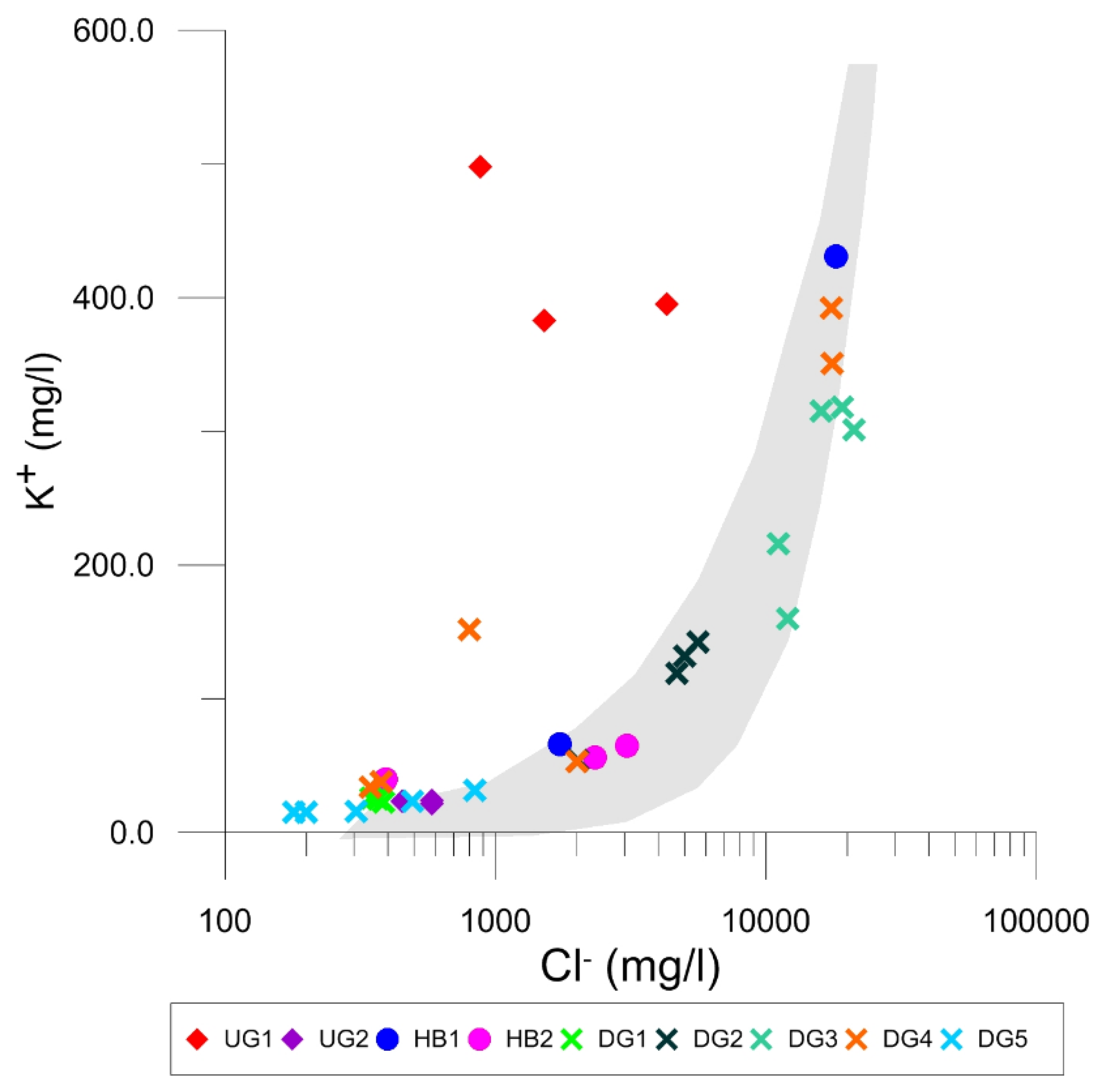
Electric conductivity (EC) and Eh measurements were done during sampling activities (

Table 1. Physical–chemical parameters, major ion concentration values, groundwater and nitrogen-stable isotopes results for groundwater sampled via MLS monitoring wells (November 2011–April 2012), rainfall and urban water. Alphabetical order indicates increasing sampling depth.

Samples ID	Elevation (m a.s.l.)	EC (μS/cm)	Eh (mV)	Cl (mg/L)	K (mg/L)	δ18O–H2O	δD–H2O	NH4 (mg/L)	NO3 (mg/L)	NO2 (μg/L)	δ15N–NH4	δ15N–NO3	δ18O–NO3
Detection limit				0.1	0.4			0.1	0.1	10
UG1a	−3.02	7800	−24	880.0	498.0	-	-	293.8	214.0	52.12	13.8	-	-
UG1b	−7.02	10,200	−60	1510.0	383.0	-	-	245.0	93.0	29.00	10.9	-	-
UG1c	−11.02	27,400	−137	4300.0	395.0	-	-	239.0	233.0	>10	3.5	-	-
UG2a	−0.61	168	3	452.0	23.6	−5.9	−36.8	>0.1	17.0	>10	-	9.4	6.4
UG2b	−4.61	159	2	580.0	23.8	−5.2	−32.2	>0.1	8.5	>10	-	13.7	6.7
UG2c	−10.61	313	2	580.0	21.3	−6.5	−42.3	>0.1	6.9	>10	-	14.4	8.9
HB1a	−4.47	35,887	−180	1730.0	66.0	-	-	1.0	7.4	22.20	-	-	-
HB1b	−12.47	39,516	−185	18,200.0	431.0	-	-	20.1	1.1	25.00	-	-	-
HB2a	−5.18	43,800	−61	393.0	39.5	-	-	107.0	33.7	150.01	−0.9	-	-
HB2b	−9.18	45,900	−74	2340.0	56.0	-	-	190.0	67.3	134.00	−0.6	-	-
HB2c	−13.18	46,100	−95	3060.0	65.0	-	-	205.0	17.5	>10	−1.0	-	-
DG1a	−3.12	2245	276	386.0	23.0	−5.2	−32.2	6.5	2.4	25.10	14.9	-	-
DG1b	−7.12	2378	241	347.0	25.9	-	-	0.4	16.4	>10	-	45.8	26.3
DG1c	−11.12	2368	226	369.0	24.9	−5.3	−33	0.3	20.6	>10	-	39.9	22.3
DG1d	−19.12	2369	208	368.0	25.5	-	-	0.2	21.6	>10	-	39.8	20.7
DG2a	−7.52	36,523	−68	2020.0	53.8	-	-	516.0	2.2	23.04	-	-	-
DG2b	−11.52	37,412	−83	4680.0	119.0	-	-	569.0	1.2	17.30	-	-	-
DG2c	−15.52	42,631	−96	5000.0	131.9	-	-	627.0	1.9	15.00	-	-	-
DG2d	−19.52	43,203	−101	5600.0	142.4	-	-	769.0	1.2	<10	-	-	-
DG3a	−5.60	43,388	−73	12,000.0	160.0	−2.8	−17.1	12.6	>0.1	53.80	−3.9	-	-
DG3b	−9.60	50,832	−96	11,100.0	216.0	-	-	25.4	>0.1	>10	−3.8	-	-
DG3c	−13.60	50,822	−101	21,200.0	301.0	0.3	2.2	13.3	>0.1	>10	−3.9	-	-
DG3d	−17.60	50,864	−104	19,200.0	318.0	-	-	12.2	>0.1	>10	−4.9	-	-
DG3e	−21.60	49,653	−93	16,000.0	315.0	0.4	2.6	10.8	>0.1	>10	−3.2	-	-
DG4a	−2.10	2441	123	344.0	33.9	−4.8	−27.8	19.3	14.9	3040.00	11.6	32.1	18.9
DG4b	−5.10	2506	125	377.0	37.9	-	-	20.3	20.5	1520.00	8.1	29.5	15.4
DG4c	−8.10	2504	129	2000.0	53.0	−2.9	−16.9	1.8	12.9	1070.00	−	19.2	14.4
DG4d	−11.10	10,614	64	17,600.0	351.0	-	-	20.9	1.6	>10	−4.9	-	-
DG4e	−15.10	48,052	−55	800.0	152.0	-	-	31.5	4.4	>10	1.4	-	-
DG4f	−19.10	50,375	−70	17,500.0	392.0	0.2	1.5	5.9	2.0	>10	−2.8	-	-
DG5a	−4.76	4074	301	180.0	15.0	−5.2	−31.5	189.0	31.7	123.30	−0.2	15.9	9.5
DG5b	−8.76	4572	299	306.0	15.5	-	-	206.0	31.5	144.00	3.4	17.3	12.3
DG5c	−12.76	5132	263	199.0	15.3	-	-	192.0	35.4	142.21	2.3	13.4	8.2
DG5d	−16.76	28,115	68	840.0	31.5	−5.1	−30.2	107.9	30.7	135.07	−1.0	15.3	11.8
DG5e	−20.76	36,629	−25	493.0	23.4	−5.1	−29.9	60.4	22.4	149.00	−0.9	24.8	14.6
Rainfall	-	-	-	-	-	−5.0	−28.0	-	-	-	-	-	-
Urban water	-	-	-	-	-	−8.6	−51.0	-	-	-	-	-	-

). Electrical conductivity, which provides information about salinity patterns, varied from minimum values of 159 µS/cm in the upgradient areas to values greater than 50,000 µS/cm near the coastline. Some salinity stratification toward high EC values with depth is observed in the monitoring wells DG4 and DG5 (Table 1). The highest EC values are associated with the influence of seawater and potentially the contribution of salts from fertilizer plants. Eh values, which give information about aquifer redox conditions, range between −185 mV and 300 mV and most of the values are in the negative range, indicating that the groundwater is under anaerobic and reducing conditions.

4.2. Cl⁻ and K⁺ Concentration Patterns

Cl⁻ concentration ranges between 180.0 mg/L and 20,000.0 mg/L, and K⁺ between 15.0 mg/L and 500.0 mg/L. The high concentrations of K⁺ and Cl⁻ are associated with fertilizers and seawater, respectively, so the relationship between K⁺ and Cl^- concentrations for the selected MLS (Figure 2) has been used for a preliminary evaluation of the influence of different contributions (local aquifer, seawater and sewage leaking) on groundwater hydrochemistry. In Figure 2, the mixing area between the background groundwater and seawater is also plotted to visualise the unreactive mixing between the two end-members; a mixing area is depicted instead of a mixing line to account for the variability of both K⁺ and Cl⁻ in the end-members.

The upgradient samples, representing the background conditions (UG2), correspond to the lower end member; the higher end-members are represented by some samples of monitoring wells HB1 and DG4. Most of the samples fall inside the mixing area, underlining the great variability in groundwater composition for this part of the aquifer, as confirmed by the wide range of electrical conductivity values. Inside the mixing area it is also possible to identify two different clusters of downgradient monitoring wells: the first one represented by DG3 and partially DG4 (deep depth), and the second one by DG1, DG5 and the remaining samples of DG4 (shallow depth). The first cluster is characterised by relatively high concentrations of both ions, suggesting a clear influence of seawater intrusion, confirmed by the electrical conductivity values; instead, the second cluster of downgradient MLS has relatively low K⁺ and Cl⁻ concentrations and lower electrical conductivity values, suggesting that the aquifer is locally recharged by leaking sewer pipelines. In addition, the flow and transport model simulations for this area of the site required a recharge amount of 200 mm/year near the sewer pipelines [14], as opposed to the rest of the site, where approximately 80 mm/year were necessary to calibrate the numerical model [28]. The most significant exception from the mixing pattern was observed in monitoring well UG1, which is characterised by a high K⁺ concentration, marking a distinct trend that could be associated with fertilizer leaching (possibly N–P–K fertilizers) (see Figure 1).

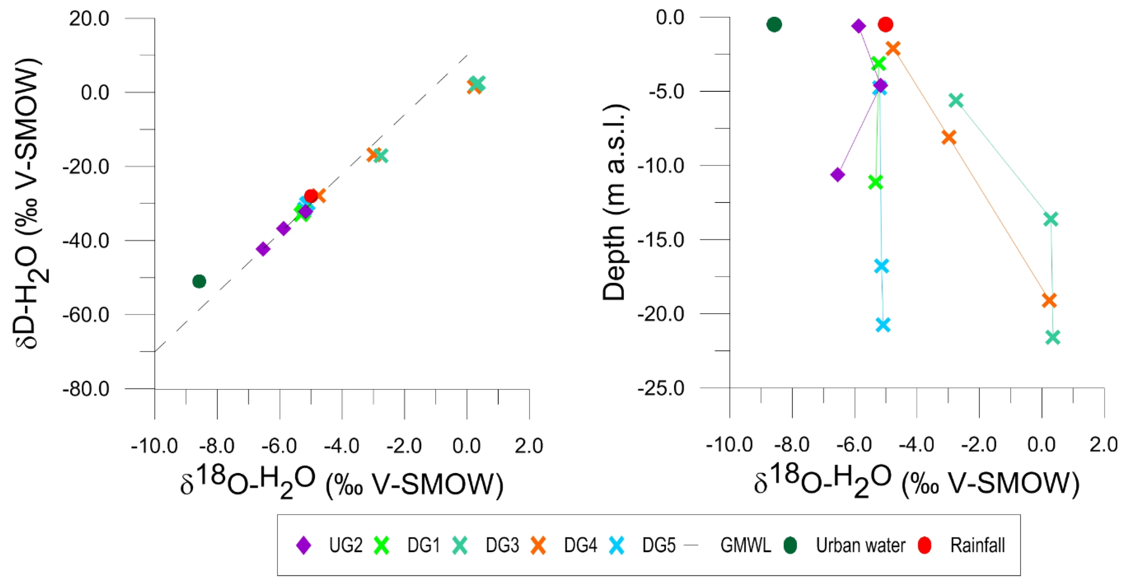
4.3. Stable Isotope Data

Groundwater isotope data have been used to further illustrate the effect of seawater intrusion and local and urban recharge. Figure 3 (left panel) shows that most of the collected samples fall along the Global Meteoric Water Line (GMWL). Monitoring wells UG2, DG1 and DG5 are characterised by an isotopic signal similar to rainfall (local recharge), with values ranging between −6.5% and −5.1% for δ¹⁸O and between −42.3% and −29.9% for δD. Groundwater with isotope values over −20.0% for δD and −2.0% for δ¹⁸O is separate from the GMWL and follows a mixing line with the seawater composition. Monitoring wells DG3 and DG4 clearly show this enrichment trend in both δ¹⁸O and δD, confirming the influence of seawater intrusion, as already suggested by Cl^- concentration and electrical conductivity values. The effect of seawater intrusion on groundwater isotopic composition is also highlighted in Figure 3 (right plot), showing the vertical profiles of δ¹⁸O for the same monitoring wells. For DG3 and DG4, it is evident that the isotopic signal changes with depth, starting from depleted δ¹⁸O values in the shallower part of the aquifer and moving to more enriched values, having an isotopic signal like seawater, in the deeper part.

4.4. Nitrogen Pollution Sources and Degradation Processes Characterisation

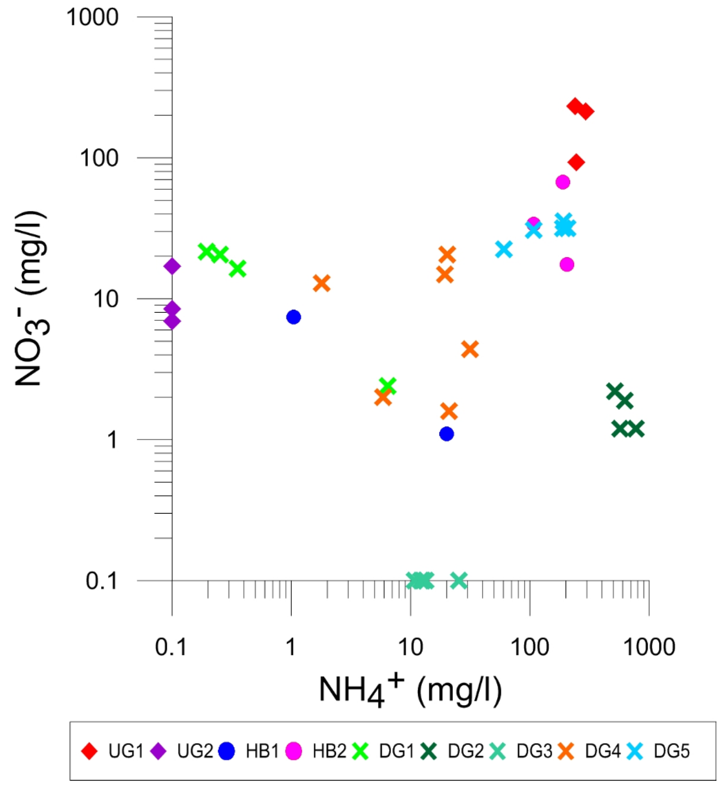
4.4.1. Concentration Patterns for Nitrogen Species and Coliforms

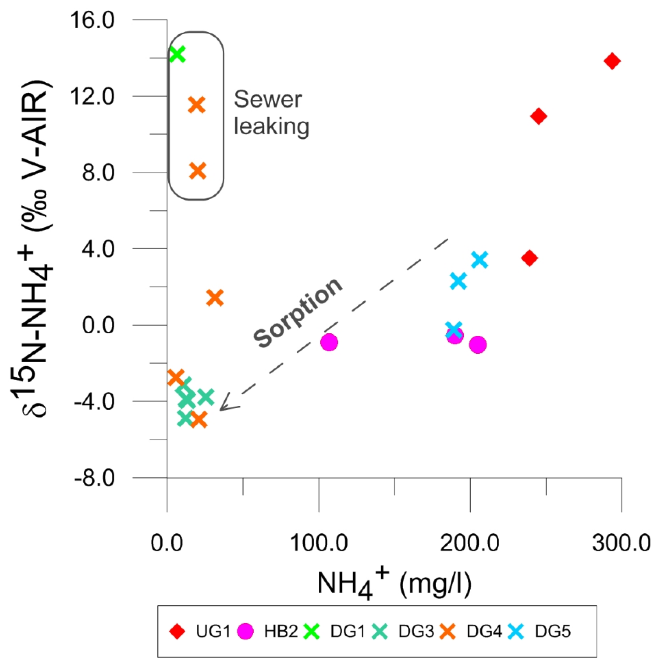
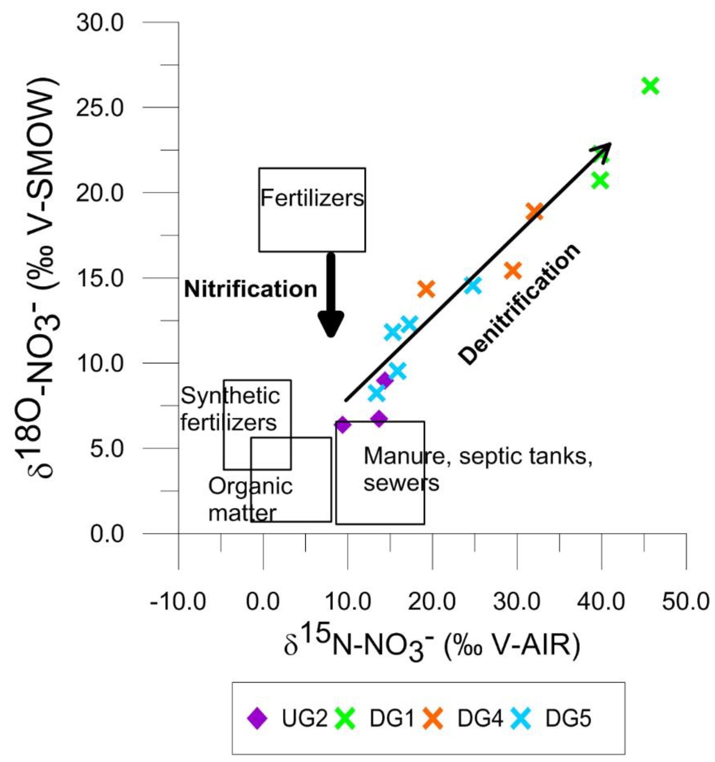
The concentration data show values ranging between 0.1 mg/L and 769.0 mg/L for NH₄⁺ and 0.1 mg/L and 233 mg/L for NO₃⁻ (Table 1). NO₂⁻ has negligible concentration in most of the samples (<10 µg/L), except in well DG4, which shows between 1.07 to 3.04 mg/L. These relative high nitrite concentrations could be associated with the partial nitrification of ammonium, associated with leakage of the sewage pipeline. The highest NH₄⁺ values are observed in well DG2 (516.0–769.0 mg/L) and could be associated with leakage of the sewage line and/or could be part of the fertilizer plume. This monitoring well is characterised by a low NO₃⁻ concentration (1.2–2.2 mg/L). The highest NH₄⁺ and NO₃⁻ concentration values are observed in well UG1, located downgradient to the fertilizer storage building and clearly related to fertilizer leakage from this facility. Background concentrations of NO₃⁻ are usually very low, with an average value of 2.5 mg/L, while NH₄⁺ is usually present at higher concentrations, with an average value of 6.5 mg/L [14].

The relationship between NH₄⁺ and NO₃⁻ concentrations in the selected MLS monitoring wells (Figure 4) highlights the coexistence of both nitrogen species in almost all the investigated monitoring wells. The existence of ammonium is associated with the partial nitrification of ammonium in the shallow unsaturated and saturated aerobic zone and the general reducing conditions of the groundwater in the aquifer. The coexistence of NH₄⁺ and NO₃⁻ in groundwater is well represented by MLS-UG1, which has high concentrations of both species between 100 and 200 mg/L, and negative Eh values (reducing conditions) recorded all along the depth profile (Table 1). UG1 is located close to the source areas (see Figure 1). The coexistence of NH₄⁺ and NO₃⁻ is also observed in other MLS samples, with a general and steep NO₃⁻ concentration decrease with respect to NH₄⁺ in MLS located near and downgradient the hydraulic barrier; this could be associated with degradation processes or mixing with other water sources depleted in NO₃⁻.

The only instances of the non-coexistence of nitrogen species are represented by monitoring wells UG2, DG2 and DG3. Specifically, monitoring well UG2, located at the fringe of the NH₄⁺ plume, shows relatively high NO₃⁻ concentrations (6.3 to 17.9 mg/L) with NH₄⁺ below detection limits, associated with positive Eh values. DG2 and DG3, located downgradient of the hydraulic barrier, show high NH₄⁺ (516.0–769.0 mg/L for DG2; 10.8–25.4 mg/L for DG3) and negligible NO₃⁻ concentrations under reducing conditions. Those samples could belong to an old plume that has already migrated downgradient with respect to the actual source area, before the installation of the pump and treat system [14]. A comparison of NH₄⁺ and NO₃⁻ concentrations does not clearly identify the different sources of pollution and reactive processes occurring at the site, but highlights the co-existence of both NH₄⁺ and NO₃⁻ in large parts of the contaminant plume.

In addition, total coliform analyses, sampled in additional monitoring wells near the hydraulic barrier (distance lower than 3 m), highlight that sewer raw waters are present in the monitoring wells located near (distance between 10 and 20 m) the sewer pipeline (

Table 2. Total coliforms detection via Most Probable Number analysis, from Sbarbati et al. [19]. Monitoring wells and pumping wells locations are showed in Figure 1 (except the upgradient monitoring well).

Sample Name	Value (MPN/100 mL)
Upgradient monitoring well	Below detection limits
Sewer pipeline	<100,000
Monitoring well 1 at the hydraulic barrier	145
Monitoring well 2 at the hydraulic barrier	300
Monitoring well 3 at the hydraulic barrier	8719
Pumping well 1 of the hydraulic barrier	Below detection limits
Pumping well 2 of the hydraulic barrier	Below detection limits
Pumping well 3 of the hydraulic barrier	Below detection limits

). The locations of sampling point are shown in Figure 1. The three corresponding pumping wells have coliform content below the detection limits due to the large amount of groundwater gathered from the lower layers of the aquifer where the pumps are located. The upgradient monitoring well, as expected, displays total coliforms below the detection limits.

Based on the information gained by major ion concentration values, groundwater isotopes analyses and total coliform analyses, it is evident that different water sources and nitrogen sources are active at the site. Additional insights regarding nitrogen sources and processes that affect nitrogen species in groundwater can be provided by the nitrogen isotopes analysis, performed on seven MLS (UG1, UG2, HB2, DG1, DG3, DG4, DG5).

4.4.2. Isotope Data on NH₄⁺ and NO₃⁻

The isotope composition of the NH₄⁺ and NO₃⁻ is controlled by the isotopic composition of the sources and transformation processes such as nitrification, denitrification and anammox [5,25,40,41]. The NO₃⁻ isotopes data at the site show a wide range of values ranging between +9.4 and +45.8% and +6.4 and +26.3% for δ¹⁵N–NO₃⁻ and δ¹⁸O–NO₃, respectively (Table 1). These values are much higher than the literature values for fertilizer and sewage [40] at the site, indicating that NO₃⁻ is been affected by an attenuation process. The enrichment trend observed for δ¹⁵N–NO₃⁻ and δ¹⁸O–NO₃⁻ (Figure 5) is typically associated with denitrification [42], which is possibly due to the reducing condition of the groundwater. Data from UG2, DG1, DG4 and DG5 monitoring wells show that NO₃⁻ in the aquifer is affected by different degrees of denitrification. The enriched δ¹⁵N pattern in residual NO₃⁻ cannot rule out anammox also being involved in degradation processes at the site [8,19,42]. NH₄⁺ also shows extremely variable δ¹⁵N–NH₄⁺ values, ranging from −4.9 to +14.9% (Table 1). The most enriched (positive) δ¹⁵N–NH₄⁺ values are observed downgradient of the fertilizer storage building (UG1), which is also characterised by the highest concentration of NH₄⁺ and NO₃⁻, and in the downgradient area near the coastline at the shallow depth in DG1 and DG4 wells, which are characterised by NH₄⁺ and NO₃⁻ concentrations less than 20.0 mg/L (Table 1). The most depleted δ¹⁵N–NH₄⁺ concentrations are observed in some downgradient wells, HB2, DG3 and DG5, which showed comparable NH₄⁺ concentrations to UG1 in the case of the DG5 well (Table 1).

The relationship between δ¹⁵N–NH₄⁺ and NH₄⁺ concentrations has been used to evaluate the origin and fate of NH₄⁺ in the aquifer (Figure 5). Considering the upgradient area and taking into account that NH₄⁺ fertilizers range between −7.4 and +6.6% [40], the highly enriched δ¹⁵N–NH₄⁺ values correlated with high concentrations of NH₄⁺ and NO₃⁻ at UG1 indicate that partial nitrification should be responsible for the enriched δ¹⁵N values in NH₄⁺. These data also show a vertical stratification, with enriched δ¹⁵N–NH₄⁺ values (+10.8 and +13.8%) observed at shallow depths and more depleted values (+3.5%) at the deepest depths. It is well documented that nitrification tends to enrich the remaining NH₄⁺ in δ¹⁵N [40,44]. The effect of partial nitrification on the isotopic composition of the NH₄⁺ was also observed in the shallow part of a septic system plume [8]. The other process that can isotopically enrich NH₄⁺ is annamox [13,41], but, unfortunately, the isotope data for NO₃⁻, which could also provide evidence about the role of anammox in NH₄⁺ transformation in one of the source zones, are not available at UG1.

Highly enriched δ¹⁵N–NH₄⁺ values are also observed in the shallow part of the aquifer at wells DG1 and DG4, located below the hydraulic barrier and the sewage line (see Table 1 and Figure 6). Low values of 6.5 and 2.4 mg/L for NH₄⁺ and NO₃⁻ are observed in DG1. Comparable concentrations of NH₄⁺ and NO₃⁻ in the range of 14 to 20 mg/L are observed at DG4 and NO₃⁻ is also characterised by enriched δ¹⁵N–NO₃⁻ and δ¹⁸O–NO₃⁻ values, associated with denitrification and anammox processes [42]. Concerning the most depleted δ¹⁵N–NH₄⁺ values (−4.9 and +1.4%), these are observed at all depths in DG3 and DG5 and in the deepest depth at DG4 in the downgradient area. The groundwater was characterised by less than 25.4 mg/L of NH₄⁺ and no NO₃⁻ in the case of DG3, 1.8 to 20.9 mg/L for NH₄⁺ and less than 20.5 mg/L of NO₃⁻ in DG4. DG5 is characterised by high NH₄⁺ (60.4 and 206.0 mg/L) and relatively high NO₃⁻ (22.4 and 35.4 mg/L). The high NH₄⁺ concentration observed at DG5 is comparable to the high concentration observed in UG1 in the source zone. These depleted δ¹⁵N–NH₄⁺ values cannot represent sewage nitrogen since this nitrogen is characterised by δ¹⁵N values between +4.0 and +6.0% [8]. This type of δ¹⁵N–NH₄⁺ value is characteristic of NH₄⁺ fertilizers and could be part of an old plume that was already present before the installation of the pump and treat system about 20 years ago. One process that could be partly responsible for the depleted δ¹⁵N–NH₄⁺ values and low NH₄⁺ concentration could be adsorption. It is well documented that during this process the remaining NH₄⁺ gets depleted in δ¹⁵N [45]. Looking at the data in Figure 6, decreasing NH₄⁺ concentrations seem to be correlated with a trend toward negative δ¹⁵N–NH₄⁺ values (grey dashed arrow). The occurrence of adsorption at the study site is supported by the high cation exchange capacity of the aquifer sediments [14]. Dilution and dispersion processes could also be partially responsible for the decreasing trend in NH₄⁺ concentrations. However, it is difficult to explain the depleted δ¹⁵N–NH₄⁺ values accompanied by a high concentration of NH₄⁺ observed at DG5 based only on adsorption. It is important to highlight that NO₃⁻ coexists with NH₄⁺ at DG5 and NO₃⁻ samples were very enriched in δ¹⁵N–NO₃⁻ and δ¹⁸O–NO₃⁻, indicating that NO₃⁻ was affected by denitrification. Thus, a more plausible theory to explain the depleted δ¹⁵N–NH₄⁺ values is that the NH₄⁺ and NO₃⁻ were both part of an old fertilizer plume that was already well developed before the installation of the pump and treat system at the site.

The other group, which is plotted in a different field to the rest of the samples, is formed by three samples (shallow depths at DG1 and DG4, Table 1) with NH₄⁺ concentrations of 6.5 mg/L (DG1) and around 20.9 mg/L (DG4) and highly positive δ¹⁵N–NH₄⁺ values (grey box in Figure 6) that could be ascribable to the partial nitrification of NH₄⁺ and also to anammox [46]. NO₃⁻ is also present at concentrations similar to NH₄⁺ in these monitoring wells (Table 1). The NO₃⁻ in DG4 also showed highly enriched δ¹⁵N–NO₃⁻ and δ¹⁸O–NO₃⁻ values (see Table 1 and Figure 5), indicating that NO₃⁻ has been affected by denitrification and was involved in anammox processes [46]. These monitoring wells are located downgradient to the sewer pipeline and the groundwater stable isotopes data clearly show the influence of local recharge (Table 1), indicating that the nitrogen species can be associated with the leakage of sewage pipelines. Therefore, from nitrogen-stable isotopes analyses we have identified the main degradation processes acting at the site, namely partial nitrification, denitrification, adsorption and anammox. In addition, the coexistence of NH₄⁺ and NO₃⁻ at elevated concentrations in most of the analysed MLS monitoring wells is also favoured by the general reducing condition of the aquifer and the fast groundwater flow field. The latter allows the transport of oxidised species like NO₃⁻ from the source (located in the vadose zone) into reducing zones within the aquifer, further triggering denitrification reactions.

5. Conclusions

The results of this study show that the combined use of hydrochemical, stable isotopes data and microbial analyses have provided valuable information to evaluate the pollutant sources and processes that affect reactive nitrogen species in an industrial coastal aquifer. The installation of the pump and treat system has significantly changed the natural flow system and the behaviour of contaminant plumes in the aquifer. The main focus of this study was to understand the processes that govern the nitrogen dynamics in the aquifer. The chemical and stable isotope data in groundwater show the influence of recharge and the occurrence of seawater intrusion in areas near the coastline. A key feature of the study site is the coexistence of NH₄⁺ and NO₃⁻. Redox parameter data (Eh) show that groundwater is under reducing conditions in most parts of the aquifer and flow velocity is elevated due to the pumping wells’ remediation system. The fast groundwater flow field is one of the reasons for the coexistence of NH₄⁺ and NO₃⁻ in groundwater, since both compounds can be mobilised in the reducing zone of the aquifer. The highly enriched δ¹⁵N–NH₄⁺ values (+13.8 and +14.9%) observed at the site are associated with partial nitrification of NH₄⁺, but anammox could also be partially responsible for these values. The NO₃⁻ isotopes data showed that NO₃⁻ is attenuated by denitrification, but anammox is also involved as an attenuation process for NO₃⁻. The other feature of the site is the existence of NH₄⁺, characterised by very depleted δ¹⁵N–NH₄⁺ values (+1.4 and −4.9%). Based on the isotope and concentration patterns at the site, it is postulated that the depleted δ¹⁵N–NH₄⁺ values represent the remnant of an old plume that was developed before the initiation of pumping by the hydraulic barrier about 20 years ago. The effect of adsorption on the isotopic composition of NH₄⁺ also cannot be overlooked since there is evidence of NH₄⁺ adsorption in sediments at the site. Due to the complexities of the nitrogen cycle disturbed by pumping wells, the effect of leakage from septic pipelines, in spite of the presence of coliforms, could not be resolved based on the isotope data on nitrogen compounds, except for one spot where the groundwater stable isotopes indicated local recharge, probably associated with leakage of the sewage pipelines. Summarising, the chemical and isotopic data have shown that partial nitrification of NH₄⁺, denitrification of NO₃⁻ and anammox have been involved in the transformation and attenuation of NH₄⁺ and NO₃⁻ at the study site. Evidence of the existence of an old fertilizer plume was also found. This study has clearly shown that a multidisciplinary approach is required to evaluate nitrogen cycling in industrial sites affected by multiple sources of contamination and seawater intrusion.

References

1. Böhlke, J.K.; Smith, R.L.; Miller, D.N. Ammonium transport and reaction in contaminated groundwater: Application of isotope tracers and isotope fractionation studies. Water Resour. Res. 2006, 42, W05411. [Google Scholar] [CrossRef]
2. Brauns, B.; Bjerg, P.L.; Song, X.; Jakobsen, R. Field scale interaction and nutrient exchange between surface water and shallow groundwater in the Baiyang Lake region, North China Plain. J. Environ. Sci. 2016, 45, 60–75. [Google Scholar] [CrossRef] [PubMed] [Green Version]
3. Zhang, Y.; Li, F.; Zhang, Q.; Li, J.; Liu, Q. Tracing nitrate pollution sources and transformation in surface-and ground-waters using environmental isotopes. Sci. Total Environ. 2014, 490, 213–222. [Google Scholar] [CrossRef] [PubMed]
4. Best, A.; Arnaud, E.; Parker, B.; Aravena, R.; Dunfield, K. Effects of glacial sediment type and land use on nitrate patterns in groundwater. Groundw. Monit. Remediat. 2015, 35, 68–81. [Google Scholar] [CrossRef]
5. Di Lorenzo, T.; Brilli, M.; Del Tosto, D.; Galassi, D.M.; Petitta, M. Nitrate source and fate at the catchment scale of the Vibrata River and aquifer (central Italy): An analysis by integrating component approaches and nitrogen isotopes. Environ. Earth Sci. 2012, 67, 2383–2398. [Google Scholar] [CrossRef]
6. Petitta, M.; Fracchiolla, D.; Aravena, R.; Barbieri, M. Application of isotopic and geochemical tools for the evaluation of nitrogen cycling in an agricultural basin, the Fucino Plain, Central Italy. J. Hydrol. 2009, 372, 124–135. [Google Scholar] [CrossRef]
7. Sebilo, M.; Mayer, B.; Nicolardot, B.; Pinay, G.; Mariotti, A. Long-term fate of nitrate fertilizer in agricultural soils. Proc. Natl. Acad. Sci. USA 2013, 110, 18185–18189. [Google Scholar] [CrossRef] [PubMed] [Green Version]
8. Caschetto, M.; Robertson, W.; Petitta, M.; Aravena, R. Partial nitrification enhances natural attenuation of nitrogen in a septic system plume. Sci. Total Environ. 2018, 625, 801–808. [Google Scholar] [CrossRef] [PubMed]
9. Roehrdanz, P.R.; Feraud, M.; Lee, D.G.; Means, J.C.; Snyder, S.A.; Holden, P.A. Spatial models of sewer pipe leakage predict the occurrence of wastewater indicators in shallow urban groundwater. Environ. Sci. Technol. 2017, 51, 1213–1223. [Google Scholar] [CrossRef] [PubMed]
10. Yang, Y.Y.; Toor, G.S. δ15N and δ18O reveal the sources of nitrate-nitrogen in urban residential stormwater runoff. Environ. Sci. Technol. 2016, 50, 2881–2889. [Google Scholar] [CrossRef] [PubMed]
11. Jiao, J.J.; Wang, Y.; Cherry, J.A.; Wang, X.; Zhi, B.; Du, H.; Wen, D. Abnormally high ammonium of natural origin in a coastal aquifer-aquitard system in the Pearl River Delta, China. Environ. Sci. Technol. 2010, 44, 7470–7475. [Google Scholar] [CrossRef] [PubMed]
12. Mastrocicco, M.; Giambastiani, B.M.S.; Colombani, N. Ammonium occurrence in a salinized lowland coastal aquifer (Ferrara, Italy). Hydrol. Processes 2013, 27, 3495–3501. [Google Scholar] [CrossRef]
13. Clark, I.; Timlin, R.; Bourbonnais, A.; Jones, K.; Lafleur, D.; Wickens, K. Origin and fate of industrial ammonium in anoxic ground water—15N evidence for anaerobic oxidation (anammox). Groundw. Monit. Remediat. 2008, 28, 73–82. [Google Scholar] [CrossRef]
14. Colombani, N.; Mastrocicco, M.; Prommer, H.; Sbarbati, C.; Petitta, M. Fate of arsenic, phosphate and ammonium plumes in a coastal aquifer affected by saltwater intrusion. J. Contam. Hydrol. 2015, 179, 116–131. [Google Scholar] [CrossRef] [PubMed]
15. Krause, S.; Heathwaite, L.; Binley, A.; Keenan, P. Nitrate concentration changes at the groundwater-surface water interface of a small Cumbrian river. Hydrol. Processes 2009, 23, 2195–2211. [Google Scholar] [CrossRef]
16. Chen, S.; Ling, J.; Blancheton, J.P. Nitrification kinetics of biofilm as affected by water quality factors. Aquac. Eng. 2006, 34, 179–197. [Google Scholar] [CrossRef]
17. Lansdown, K.; Heppell, C.M.; Trimmer, M.; Binley, A.; Heathwaite, A.L.; Byrne, P.; Zhang, H. The interplay between transport and reaction rates as controls on nitrate attenuation in permeable, streambed sediments. J. Geophys. Res. Biogeosci. 2015, 120, 1093–1109. [Google Scholar] [CrossRef] [Green Version]
18. Snider, D.M.; Spoelstra, J.; Schiff, S.L.; Venkiteswaran, J.J. Stable oxygen isotope ratios of nitrate produced from nitrification: 18O-labeled water incubations of agricultural and temperate forest soils. Environ. Sci. Technol. 2010, 44, 5358–5364. [Google Scholar] [CrossRef] [PubMed]
19. Sbarbati, C.; Colombani, N.; Mastrocicco, M.; Aravena, R.; Petitta, M. Performance of different assessment methods to evaluate contaminant sources and fate in a coastal aquifer. Environ. Sci. Pollut. Res. 2015, 22, 15536–15548. [Google Scholar] [CrossRef] [PubMed]
20. Philips, S.; Laanbroek, H.J.; Verstraete, W. Origin, causes and effects of increased nitrite concentrations in aquatic environments. Rev. Environ. Sci. Biotechnol. 2002, 1, 115–141. [Google Scholar] [CrossRef] [Green Version]
21. Caschetto, M.; Colombani, N.; Mastrocicco, M.; Petitta, M.; Aravena, R. Nitrogen and sulphur cycling in the saline coastal aquifer of Ferrara, Italy. A multi-isotope approach. Appl. Geochem. 2017, 76, 88–98. [Google Scholar] [CrossRef] [Green Version]
22. Ding, J.; Xi, B.; Xu, Q.; Su, J.; Huo, S.; Liu, H.; Yu, Y.; Zhang, Y. Assessment of the sources and transformations of nitrogen in a plain river network region using a stable isotope approach. J. Environ. Sci. 2015, 30, 198–206. [Google Scholar] [CrossRef] [PubMed]
23. Ma, Z.; Yang, Y.; Lian, X.; Jiang, Y.; Xi, B.; Peng, X.; Yan, K. Identification of nitrate sources in groundwater using a stable isotope and 3DEEM in a landfill in Northeast China. Sci. Total Environ. 2016, 563, 593–599. [Google Scholar] [CrossRef] [PubMed]
24. Martínez, D.; Moschione, E.; Bocanegra, E.; Galli, M.G.; Aravena, R. Distribution and origin of nitrate in groundwater in an urban and suburban aquifer in Mar del Plata, Argentina. Environ. Earth Sci. 2014, 72, 1877–1886. [Google Scholar] [CrossRef]
25. Minet, E.P.; Goodhue, R.; Meier-Augenstein, W.; Kalin, R.M.; Fenton, O.; Richards, K.G.; Coxon, C.E. Combining stable isotopes with contamination indicators: A method for improved investigation of nitrate sources and dynamics in aquifers with mixed nitrogen inputs. Water Res. 2017, 124, 85–96. [Google Scholar] [CrossRef] [PubMed]
26. Puig, R.; Soler, A.; Widory, D.; Mas-Pla, J.; Domènech, C.; Otero, N. Characterizing sources and natural attenuation of nitrate contamination in the Baix Ter aquifer system (NE Spain) using a multi-isotope approach. Sci. Total Environ. 2017, 580, 518–532. [Google Scholar] [CrossRef] [PubMed]
27. Wells, N.S.; Hakoun, V.; Brouyère, S.; Knöller, K. Multi-species measurements of nitrogen isotopic composition reveal the spatial constraints and biological drivers of ammonium attenuation across a highly contaminated groundwater system. Water Res. 2016, 98, 363–375. [Google Scholar] [CrossRef] [PubMed] [Green Version]
28. Mastrocicco, M.; Colombani, N.; Sbarbati, C.; Petitta, M. Assessing the effect of saltwater intrusion on petroleum hydrocarbons plumes via numerical modelling. Water Air Soil Pollut. 2012, 223, 4417–4427. [Google Scholar] [CrossRef]
29. Mastrocicco, M.; Sbarbati, C.; Colombani, N.; Petitta, M. Efficiency verification of a horizontal flow barrier via flowmeter tests and multilevel sampling. Hydrol. Processes 2013, 27, 2414–2421. [Google Scholar] [CrossRef]
30. Epstein, S.; Mayeda, T. Variation of O-18 content of waters from natural sources. Geochim. Cosmichim. Acta 1953, 4, 213–224. [Google Scholar] [CrossRef]
31. Longinelli, A.; Selmo, E. Isotopic composition of precipitation in Italy: A first overall map. J. Hydrol. 2003, 270, 75–88. [Google Scholar] [CrossRef]
32. Coleman, M.L.; Sheppard, T.J.; Durham, J.J.; Rouse, J.E.; Moore, G.R. Reduction of water with zinc for hydrogen isotope analyses. Anal. Chem. 1982, 54, 993–995. [Google Scholar] [CrossRef]
33. Brooks, P.D.; Stark, J.M.; McInteer, B.B.; Preston, T. Diffusion method to prepare soil extracts for automated nitrogen-15 analysis. Soil Sci. Soc. Am. J. 1989, 53, 1707–1711. [Google Scholar] [CrossRef]
34. Sørensen, P.; Jensen, E.S. Sequential diffusion of ammonium and nitrate from soil extracts to a polytetrafluoroethylene trap for 15N determination. Anal. Chim. Acta 1991, 252, 201–203. [Google Scholar] [CrossRef]
35. Silva, S.R.; Kendall, C.; Wilkison, D.H.; Ziegler, A.C.; Chang, C.C.Y.; Avanzino, R.J. A new method for collection of nitrate from fresh water and the analysis of nitrogen and oxygen isotope ratios. J. Hydrol. 2009, 228, 22–36. [Google Scholar] [CrossRef]
36. Casciotti, K.L.; Sigman, D.M.; Hastings, M.; Böhlke, J.K.; Hilkert, A. Measurement of the oxygen isotopic composition of nitrate in seawater and freshwater using the denitrifier method. Anal. Chem. 2002, 74, 4905–4912. [Google Scholar] [CrossRef] [PubMed]
37. Rock, L.; Ellert, B.H. Nitrogen-15 and oxygen-18 natural abundance of potassium chloride extractable soil nitrate using the denitrifier method. Soil Sci. Soc. Am. J. 2007, 71, 355–361. [Google Scholar] [CrossRef] [Green Version]
38. Sigman, D.M.; Casciotti, K.L.; Andreani, M.; Barford, C.; Galanter, M.; Böhlke, J.K. A bacterial method for the nitrogen isotopic analysis of nitrate in seawater and freshwater. Anal. Chem. 2002, 73, 4145–4153. [Google Scholar] [CrossRef]
39. Hurley, M.A.; Roscoe, M.E. Automated statistical-analysis of microbial enumeration by dilution series. J. Appl. Microbiol. 1983, 55, 159–164. [Google Scholar] [CrossRef]
40. Aravena, R.; Mayer, B. Isotopes and Processes in the Nitrogen and Sulfur Cycles. In Environmental Isotopes in Biodegradation and Bioremediation; CRC Press/Lewis: Boca Raton, FL, USA, 2010; pp. 203–246. ISBN 9781566706612. [Google Scholar]
41. Robertson, W.D.; Moore, T.A.; Spoelstra, J.; Li, L.; Elgood, R.J.; Clark, I.D.; Schiff, S.L.; Aravena, R.; Neufeld, J.D. Natural attenuation of septic system nitrogen by anammox. Groundwater 2012, 50, 541–553. [Google Scholar] [CrossRef] [PubMed]
42. Aravena, R.; Robertson, W. The use of multiple isotope tracers to evaluate denitrification in groundwater: A case study in a large septic system plume. Groundwater 1998, 36, 975–982. [Google Scholar] [CrossRef]
43. Clark, I.; Fritz, P. Environmental Isotopes in Hydrogeology; CRC Press/Lewis: Boca Raton, FL, USA, 1997; ISBN 1566702496. [Google Scholar]
44. Mariotti, A.; Germon, J.C.; Hubert, P.; Kaiser, P.; Letolle, R.; Tardieux, A.; Tardieux, P. Experimental determination of nitrogen kinetic isotope fractionation: Some principles; Illustration for the denitrification and nitrification processes. Plant Soil 1981, 62, 413–430. [Google Scholar] [CrossRef]
45. Karamanos, R.E.; Rennie, D.A. Nitrogen isotope fractionation during ammonium exchange reactions with soil clay. Canad. J. Soil Sci. 1978, 58, 53–60. [Google Scholar] [CrossRef]
46. Sbarbati, C. Use of an Integrated Methodological Approach to Assess Contaminant Fate and Transport in a Coastal Aquifer. Ph.D. Thesis, Sapienza University of Rome, Rome, Italy, 2013. [Google Scholar]
Figure 1. Top panel: Location map of the long screen monitoring wells used in the study including: MLS located upgradient with respect to the hydraulic barrier (diamonds), near the hydraulic barrier (circles), and downgradient with respect to the pumping wells (brown crosses), and related shallow monitoring wells sampled for coliforms analyses (brown circles with crosses). Pumping wells equivalent freshwater heads contours above sea level (blue lines). Various N pollution sources creating NH4+ and NO3 plumes (red shaded areas): sewer pipeline, Fertilizer storage buildings and NH3 plant. Red line shows the industrial site boundary. Bottom panel: Cross section A-A′ (dashed line on the top panel) representing a simplified geological profile of the unconfined aquifer. Vertical exaggeration is 1:10.
Geosciences 08 00210 g001
Figure 2. Plot of Cl versus K+ for MLS located upgradient (UG1, UG2), near (HB1, HB2) and downgradient (DG1 ÷ DG5) with respect to the hydraulic barrier (see Figure 1 for sampling site location). The grey shaded area shows the mixing between the background groundwater concentration and seawater.
Geosciences 08 00210 g002
Figure 3. δ18O–δD (left) and δ18O-depth (right) plots in samples analysed from MLS, located upgradient (UG2) and downgradient (DG1, DG3, DG4, DG5), respectively, with respect to the hydraulic barrier (see Figure 1 for sampling site location).
Geosciences 08 00210 g003
Figure 4. Plot of NH4+ versus NO3 in samples analysed from MLS located upgradient (UG1, UG2), near the hydraulic barrier (HB1, HB2) and downgradient (DG1 ÷ DG5) with respect to the hydraulic barrier (see Figure 1 for sampling site location).
Geosciences 08 00210 g004
Figure 5. Diagram of δ15N–NO3 versus δ18O–NO3 in samples analysed from MLS located upgradient (UG2) and downgradient (DG1, DG4 and DG5) with respect to the hydraulic barrier (see Figure 1 for sampling site location). Modified from Clark and Fritz [43].
Geosciences 08 00210 g005
Figure 6. Plot of NH4+ versus δ15N–NH4+ in samples analysed from MLS located upgradient (UG1), near (HB2) and downgradient (DG1, DG3, DG4, DG5), respectively, with respect to the hydraulic barrier (see Figure 1 for sampling site location).
Geosciences 08 00210 g006