Exploring the Impact of Analysis Scale on Landslide Susceptibility Modeling: Empirical Assessment in Northern Peloponnese, Greece


Department of Geography, Harokopio University, El. Venizelou 70, 17671 Athens, Greece
*
Author to whom correspondence should be addressed.
Geosciences 2018, 8(7), 261; https://doi.org/10.3390/geosciences8070261
Submission received: 23 May 2018
/
Revised: 5 July 2018
/
Accepted: 8 July 2018
/
Published: 12 July 2018
(This article belongs to the Section Natural Hazards)
Abstract
:The main purpose of this study is to explore the impact of analysis scale on the performance of a quantitative model for landslide susceptibility assessment through empirical analyses in the northern Peloponnese, Greece. A multivariate statistical model like logistic regression (LR) was applied at two different scales (a regional and a more detailed scale). Due to this scale difference, the implementation of the model was based on two landslide inventories representing in a different way the landslide occurrence (as point and polygon features), and two datasets of similar geo-environmental factors characterized by a different size of grid cells (90 m and 20 m). Model performance was tested by a standard validation method like receiver operating characteristics (ROC) analysis. The validation results in terms of accuracy (about 76%) and prediction ability (Area under the Curve (AUC) = 0.84) of the model revealed that the more detailed scale analysis is more appropriate for landslide susceptibility assessment and mapping in the catchment under investigation than the regional scale analysis.
1. Introduction
Landslides occur throughout the world, under all climatic conditions and terrains, costing billions in monetary losses and being responsible for thousands of deaths and injuries each year [1]. The expanding urbanization and development (urban activities and transportation facilities) in landslide-prone areas, in combination with the climate change of extreme meteorological events, and the high seismic activity have contributed to the increase of landslide frequency worldwide, during the last decades. In 2016, 4% of global natural hazards were associated with landslides [2], while only in the first semester of 2017, the same percentage was 11% [3]. In terms of mortality, the corresponding percentages were 5% and 25%, respectively, of the total of human life losses.
Greece can be characterized as a region highly prone and vulnerable to the occurrence of landslides [4]. Due to (a) uncontrolled or not well planned development by ignoring the engineering geological and geotechnical conditions, (b) excessive rainfall events generating high pore water pressure, and (c) strong earthquakes resulting in ground shaking, more and more areas of the country are affected by them [5,6]. Therefore, the need for reliable predictive maps is uncontested nationally, in order to mitigate the phenomenon by avoiding the hazard or reducing the potential effects.
A landslide susceptibility (LS) map gives an indication of where future landslides are likely to occur, based on the identification of areas of past landslide occurrences and areas where similar or identical physical characteristics exist [7]. These maps are currently prepared analyzing a variety of input data by either qualitative or quantitative models [8,9]. The qualitative models depend on the knowledge and previous experience of the experts (low degree of objectivity). Such models, well known and widely used, are the logical analytical models [10,11]. However, the quantitative models are based on numerical expressions of the relationship between landslide occurrence and influencing factors (high degree of objectivity). They include geotechnical engineering models [12,13], conventional statistical models of bivariate or multivariate analysis [14,15,16,17,18], as well as more advanced data mining models such as artificial neural networks, support vector machines, decision trees, and neuro-fuzzy models [19,20,21,22].
Concerning the accuracy of the outcomes produced from the LS models, the quality of available geographical input data plays a major role. One of the important—if not the most important—properties of the geographical data which highly reveals their quality is spatial resolution. For raster data structure, the spatial resolution of the data is expressed via the size of grid cells. Grid cells are the basic spatial components in which a study area is partitioned and for which a LS model is able to produce a prediction (susceptible/insusceptible). The size of grid cells can control the precision of the spatial coupling between the input landslide data and geo-environmental factor data [23]. The selection of the appropriate size mainly depends on the analysis scale. Large cells are more beneficial to small scales, whereas small cells are more beneficial to large scales.
In the last fifteen years, several studies have examined the effect of different grid cell sizes in LS assessment and mapping [23,24,25,26]. However, these studies have focused on the variations of the estimated LS, by changing the grid cell size and retaining same the analysis scale. In contrast with them, the present study examines the effect of different analysis scales on LS assessment for a catchment in northern Peloponnese (Greece). This effect was evaluated by applying a quantitative model at two different analysis scales (a regional scale of 1:250,000 and a more detailed scale of 1:50,000) with different sizes of grid cells (90 m and 20 m, respectively), and comparing the results derived from the model for these two analyses in terms of accuracy and prediction ability.
2. Study Areas
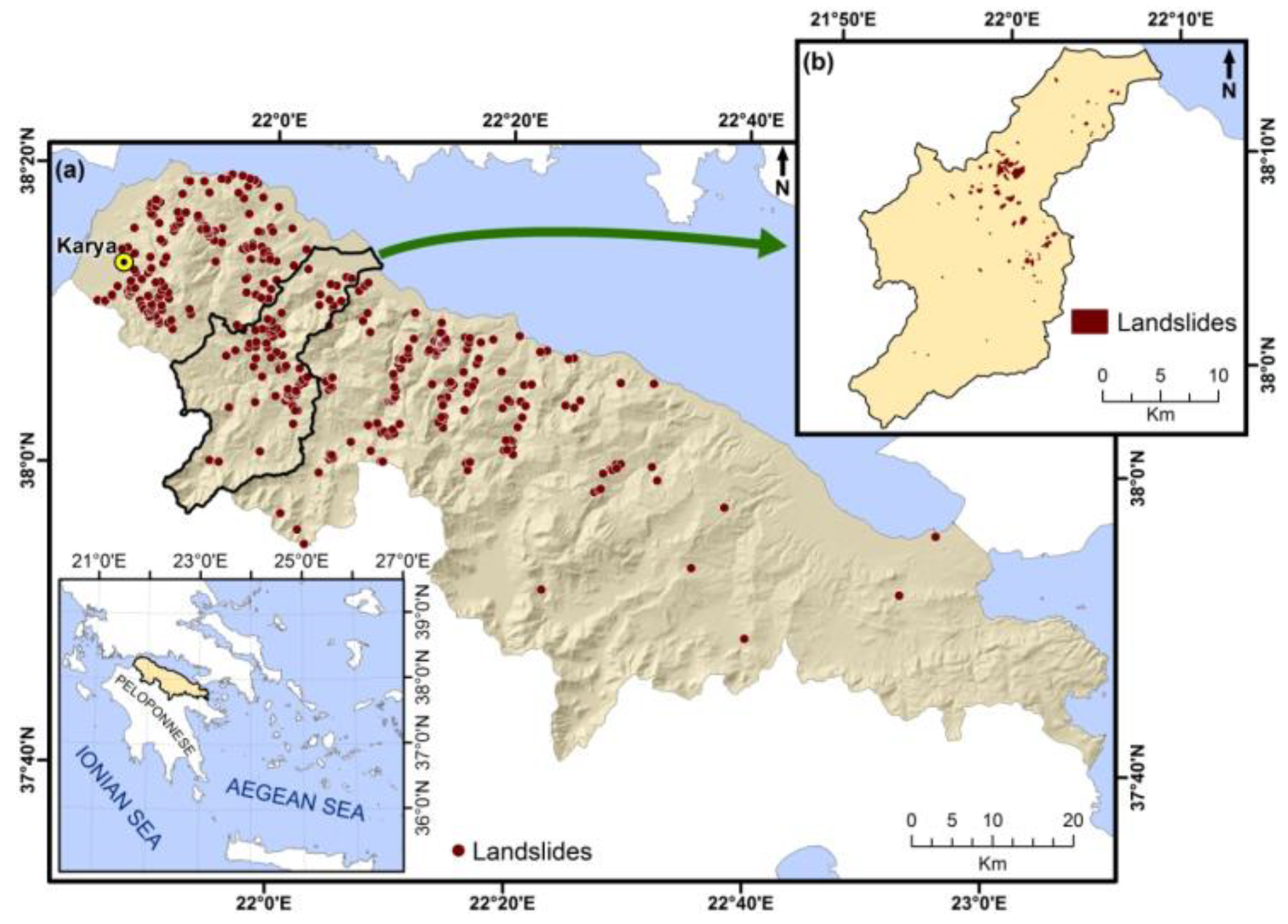
For applying the selected LS model at two different analysis scales, two study areas of different size were required. For the analysis of regional scale, a system of catchments in the northern Peloponnese was chosen as study area (Figure 1a). This area covers an extent of 3685 km2 and contains 42 catchments with some of the most important rivers of Peloponnese. One of these catchments is the (main) study area which was chosen for the analysis of more detailed scale. With an extent of 366 km2, this catchment is drained by Selinous River, the largest (with a length of 49 km) Peloponnesian river (Figure 1b).
In northern Peloponnese, agricultural areas and scrub/herbaceous vegetation are the dominant land cover types. Topographically, the presence of large and steep gorges in a significant part of its extent has to be noted. Moreover, lowland topography is detected, especially in its coastal zone. Geologically, it mainly consists of Alpine formations from three Hellenic geotectonic zones: Pindos, Tripolis, and Pelagonian zones [27]. Mostly, these formations are thickly bedded limestones, as well as conglomeratic layers. The existence of alluvial deposits in its coastal zone is also worth mentioning.
The climate is typical Mediterranean, with a hot and relatively dry summer, and a wet season during autumn, winter and spring [28]. The mean annual precipitation in northern Peloponnese ranges from 697 to 1178 mm, with the highest rainfall frequency and intensity occur during November and January. Due to these high precipitation levels, and the fact that a large part of the region consists of easily erodible geological formations, the anticipated strong relationship between precipitation and erosion can be considered as the main triggering factor for landslides.
Generally, the northern Peloponnese has experienced the occurrence of several detrimental landslide events in the past. Many villages within its boundaries have been highly damaged by these events. The most typical example is the landslide occurred in Karya, in 1962, resulting to the partial destruction of the homonym village. The village was re-sited later to a nearby geologically stable area where it is now situated [29]. Thus, considering the principle that “the past is the key to the future” [1], it is evident that slope instability is one of the most severe hazards in the region.
3. Data
In order to accomplish the LS analyses, two spatial databases—one for each of the two analysis scales—were designed and developed in GIS environment with the use of ArcGIS (ver. 10.2.2) software package.
3.1. Landslide Inventory
A landslide inventory is a dataset referring to former landslides in an area under investigation [30]. Given that, it plays a major role for recognizing factors contributing to landslide occurrence, it is considered as the most critical information in quantitative modeling for LS assessment. Landslide inventory maps may be prepared by different techniques based on the analysis scale. Smaller-scale maps may present only landslide locations, whereas larger-scale maps may identify the definite areas of landslides [31].
In this study, two landslide data sources were firstly exploited for the detection of former landslides: (a) A database about landslides in northern Peloponnese recorded by [32], covering a time period from 1906 to 2003, and (b) a web database about landslides in the northern and western parts of Peloponnese maintained by the Laboratory of Engineering Geology in the Department of Geology at the University of Patras [33], covering a time period from 1920 to 2015. Two landslide inventory maps were then created for the two different analysis scales. The first map for the regional scale analysis was obtained using the landslide location information (spatial coordinates) from the two data sources. It included 411 landslide locations, plotted as point features (Figure 1a), for the system of catchments in northern Peloponnese. The second map for the more detailed scale analysis was realized using high-resolution (Google Earth) satellite imagery interpretation, and field surveys. It referred to the Selinous catchment and contained 76 landslides whose depletion and accumulation zones were mapped together in an entire area forming a single polygon feature for each of them (Figure 1b).
Following the proposed landslide classification by [34], both point and polygon features mainly represent shallow rotational and translational slides, as well as flows. Concerning the characteristics of these landslide types, their velocity and volume vary from extremely slow (lower than 16 mm/year) to extremely rapid (higher than 5 m/s) [34] and from 200 to 6,000,000 m3, respectively. Their size also ranges from 10 to 650 m for the length and from 20 to 580 m for the width.
3.2. Geo-Environmental Factors
Landslides, like most of the natural hazards, constitute the result of the interaction between several geo-environmental factors. Theoretically, any geo-environmental factor relating to landslide phenomenon can be introduced in a LS analysis, on condition that it can be expressed in a measuring scale (continuous or categorical) and has spatial variability [35]. These factors can be subdivided into two groups: (a) The causal factors that are expected to have an effect on the landslide occurrence, and (b) the triggering factors that trigger it. Since the triggering factor data are derived from the assessment of magnitude-frequency relations for multi-temporal recorded triggering events, such as rainfalls and earthquakes, they have more utility when dealing with large areas on a small analysis scale [36]. Due to this fact and the desire for similarity between the factors in the two different scale LS analyses, only causal factors were used in the present study.
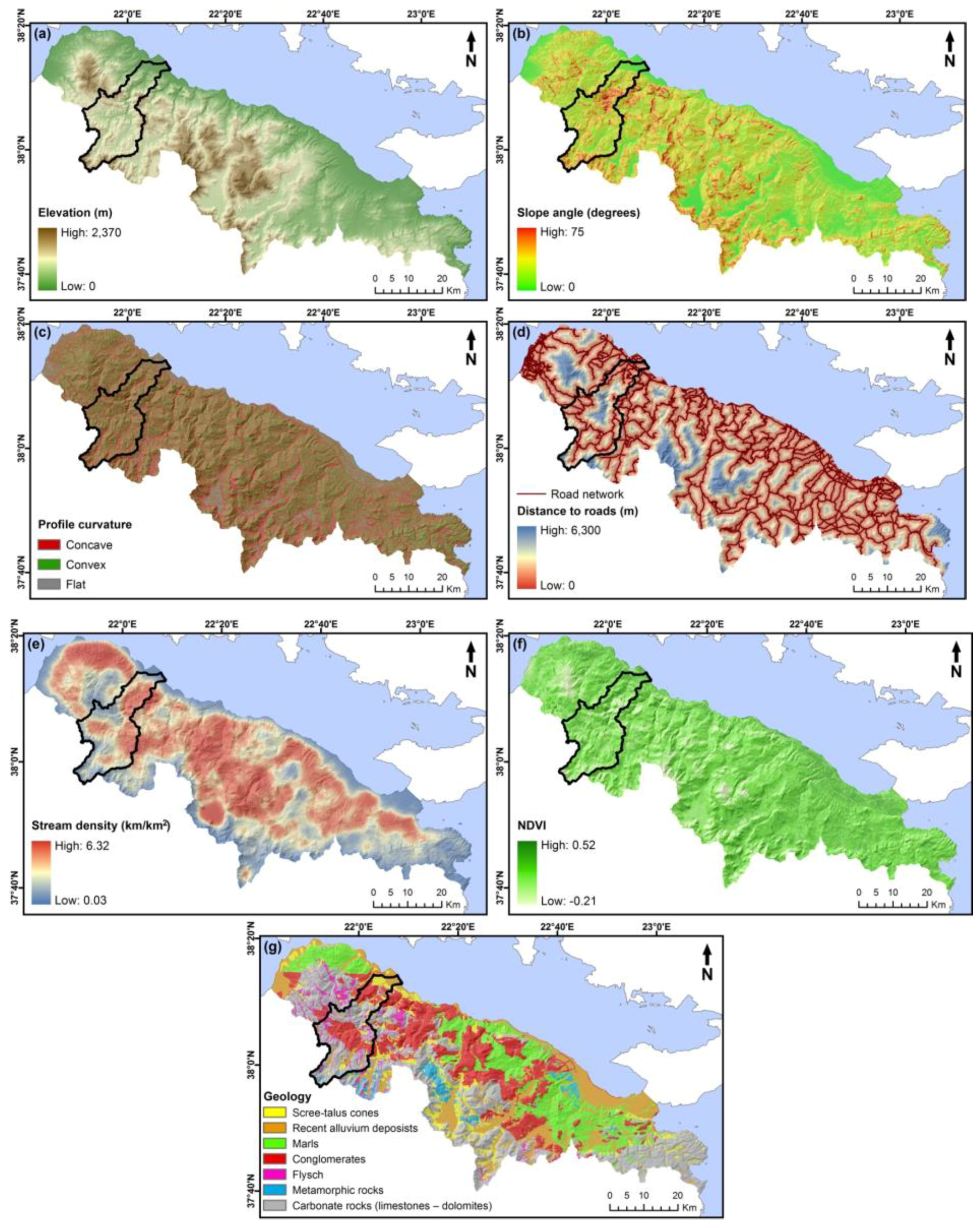
As regards the causal factors, there are no standard criteria for selecting them. Thus, the physiography of northern Peloponnese, the data availability, as well as general literature suggestions [21,26,37,38,39] were taken into account. Seven factors, such as elevation, slope angle, profile curvature, distance to roads, stream density, geology, and normalized difference vegetation index (NDVI), were selected to be included in the LS analyses.
As topography is one of the major factor types in any LS analysis, elevation, slope angle, and profile curvature factors were created. The elevation, which corresponds to the height above the mean sea level, is useful to classify the local relief and locate points of maximum and minimum heights within terrains [18]. Generally, landslides preferentially affect steeper slope portions in many different landscape settings. Therefore, an increased slope angle is correlated with an increased likelihood of failure [40]. The profile curvature shows the curvature along the vertical profile of the topography [41]. Concave areas (negative values) are also correlated with an increased likelihood of failure since, following heavy rain and thus erosion, they retain more water and sediment, and for a longer period than convex areas (positive values).
Distance of the slopes to roads is considered as a potentially significant factor on landslide occurrence. Road openings at the slope bases have negative impacts on slope stability. Stream density is the ratio of the total length of drainage network to the area of the catchment. The higher the stream density is, the lower the infiltration and the faster the mass movement will be [37]. The factors of stream density and distance to roads were created within a GIS-based analysis framework by using the proper tools. Given that different geological formations have different slope stability performances, geology is a very important factor for LS assessment [15]. Furthermore, the landslide occurrence is closely related to vegetation density. Barren slopes are more prone to landslides as compared to those with higher vegetation coverage [39]. A well-known index for vegetation density is the NDVI which is derived from the ratio (NIR − R)/(NIR + R), where NIR and R are the near-infrared and red, respectively, bands of satellite imagery data [42]. The values of this index range between −1 and +1 indicating a lack of vegetation or dense vegetation, respectively [43].
The above causal factors were organized in the relative GIS data layers as they are presented in Table 1 and Figure 2. The factors for the regional scale analysis were all converted into raster grids with cell size 90 m, whereas the factors for the more detailed scale analysis were all converted into raster grids with cell size 20 m.
4. Methodology
Logistic regression (LR) is a standard statistical model for LS assessment [16,17,18]. It is included in a category of statistical models called generalized linear models, as it allows forming a multivariate regression relation between a dependent variable and several independent variables [44]. LR is based on the basic principle that the dependent variable is generally binary, i.e., it can have only two values (for instance, 0 and 1). The independent variables act as predictors of the dependent variable and can be either continuous or categorical, or any combination of these two types.
In the case of LS assessment, the goal of LR is to find the best fitting model to describe the relationship between the absence and presence (value of 0 and 1) of landslides (dependent variable), and a set of causal factors (independent variables) [40]. The model can be expressed in its simplest form as [45]:
where P is the probability of landslide occurrence, which ranges from 0 to 1 on an S-shaped curve, and z is a linear sum of a constant and the product of the independent variables and their respective coefficients. The value of z varies from −∞ to +∞ and is calculated from the equation:
where n is the number of independent variables, xi (i = 1, 2,…, n) are the independent variables, b0 is the constant of the model, and bi (i = 1, 2,…, n) are the coefficients. The coefficient represents a measure of the association between a certain causal factor and the landslide occurrence. For a positive association the coefficient is positive, whereas for a negative association it is negative. A coefficient of or very close to 0 indicates a factor not being influential in landslide occurrence. The LR model estimates the coefficients and statistics, based on the values of independent variables and the status of the dependent variable in a sample of data, using a maximum likelihood method [46]. Using the outcomes derived from the implementation of model on the selected sample, the probability of landslide occurrence can be calculated.
The main steps of the methodology followed in both LS analyses are presented below:
- (a)
- Data sampling for the dependent variable. An important issue in the LR modeling is the sample of data used to create the dependent variable. In this study, each of the two landslide inventories was split into two separate groups: A training dataset with 80% of landslide data for the implementation of the model, and a validation dataset with 20% of landslide data for the evaluation of LS outputs. Thus, for the regional scale analysis, among the 411 landslide location points, 329 points were randomly selected as the training dataset, and the remaining 82 points events made up the validation dataset. On the other hand, for the more detailed scale analysis, among the 76 landslide polygons, 61 polygons were randomly selected as the training dataset, and the remaining 15 polygons made up the validation dataset. These polygons were then converted into points (centroids of grid cells) by tiling the entire study area (Selinous catchment) into grid cells of size 20 m. It resulted to 5140 training landslide points and 446 validation landslide points. Furthermore, for each of the two analyses, an equal number of points from the landslide-not-occurrence part of the corresponding study area was randomly selected for both the training (giving totals of 658 and 10,280 respectively, points) and validation (giving totals of 164 and 892, respectively, points) datasets. The target value of 1 was assigned to the landslide points, while the target value of 0 to the non-landslide points.
- (b)
- Preparation of independent variables. As it was mentioned above, the LR model allows the integration of both continuous and categorical independent variables. However, combining data with different measuring scales can lead to problems in the interpretation of final results [47]. The common method for resolving this issue is to normalize them. Thus, the factor data needed to be categorized and normalized in order to generate an accurate model for both analyses. The GIS-based “Natural Breaks (Jenks)” categorization was preferred for the factors with continuous values (elevation, slope angle, distance to roads, stream density, and NDVI) in both analyses, except for profile curvature factor whose categorization was executed in a manually generalized way based on its presented values. In Natural Breaks, class breaks are identified that best group similar values and that maximize the differences between classes, according to the deviations about the median [48]. Moreover, by grouping the initial categories based on their common characteristics for the regional scale analysis and preserving the initial categories for the more detailed scale analysis, the categorized geology factor was created (Figure 2). The factor data were then normalized in the range 0.1–0.9 by coding and ranking their various categories based on the relative landslide density values.
- (c)
- Creation of input database. The totals of 658 and 10,280 respectively, training points were matched with the relative normalized category values of causal factors, through a GIS-based spatial analysis tool, to create a database for each of the two analyses.
- (d)
- Multicollinearity checking. It was required to check the correlation of independent variables. The calculation of tolerance (TOL) and variance inflation factor (VIF) indexes is the most known method for this purpose [49].
- (e)
- Implementation of LR model. The databases derived from step (c), with the seven normalized causal factors as independent variables, and the presence and absence of landslide (binary target value of 0 and 1) as dependent variable were imported into the LR algorithm within the SPSS 22.2 software package.
- (f)
- Production of final LS map. After assigning coefficients to all the independent variables, a GIS-based weighted overlay was applied using Equation (2). Consequently, by inserting the output into the Equation (1), the final LS map was created for each of the two analyses. These maps were categorized into five categories (“Very Low”, “Low”, “Moderate”, “High” and “Very High” susceptibility) based on the “Natural Breaks (Jenks)” method.
- (g)
- Validation of the models. Validation is an essential process to know the accuracy and prediction ability of the LS assessment models. A validation method, named as receiver operating characteristics (ROC) analysis, has been widely applied to evaluate the overall performance of these models [50,51]. In ROC analysis, the model’s sensitivity is shown as a function of the specificity. The sensitivity refers to the percentage of positively predicted cases among the positive observations, whereas specificity refers to the percentage of negatively predicted cases among the negative observations [52]. The relationship between sensitivity and specificity is graphically represented by the ROC curve. The ROC graph consists of two axes: y-axis represents the sensitivity and x-axis represents the difference 1–specificity. Thus, high sensitivity indicates a high number of correct predictions, and high specificity (low 1−specificity) indicates a low number of incorrect predictions [53]. Among the statistics derived from ROC analysis, the area under the curve (AUC) value also plays a significant role. With a range from 0.5 to 1.0, the higher this value is, the more optimal is the model. In this study, the ROC analysis was applied for both analyses using the relative validation datasets.
5. Results
In multicollinearity checking TOL and VIF were calculated. For both analyses, these indexes were found to be greater than 0.2 for TOL and less than 10 for VIF (Table 2) revealing that there is no multicollinearity between any of the independent variables.
The model statistics and the coefficients of independent variables (Table 3) were then estimated for both analyses. The results of the LR model reveal that all causal factors are positively related to the landslide occurrence for both analyses (Table 3). For regional scale analysis, geology, NDVI, and distance to roads are found to have the strongest effect (coefficients of 8.019, 6.856 and 6.227, respectively) on landslides than the other factors. Elevation, and profile curvature are the factors with the weakest effect (coefficients of 2.007 and 2.505, respectively). On the contrary, for the more detailed scale analysis, the most important causal factors are found to be elevation, stream density, and slope angle (coefficients of 9.178, 4.796 and 4.474, respectively). Distance to roads, and NDVI are the factors with the lowest importance (coefficients of 2.258 and 2.880, respectively).
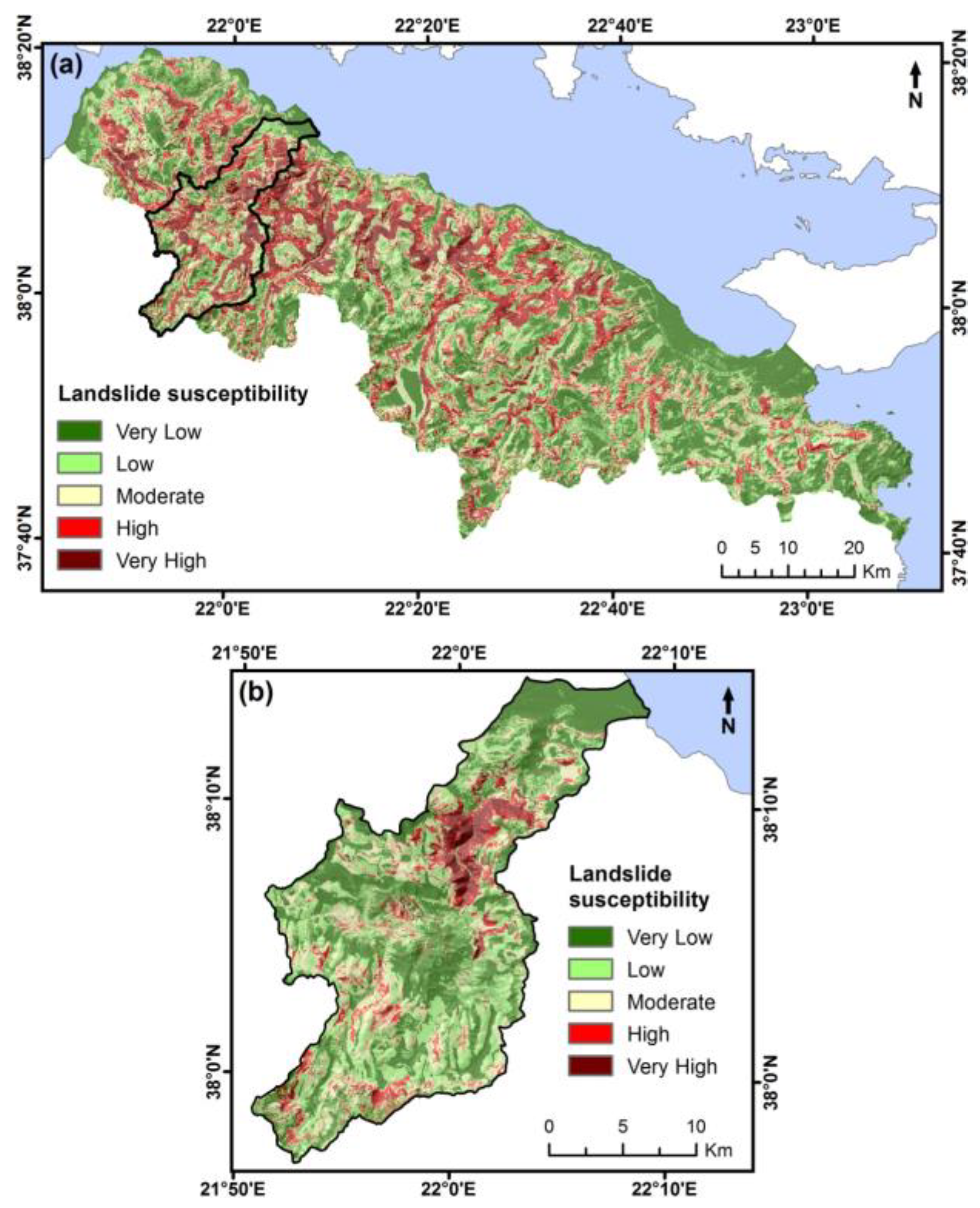
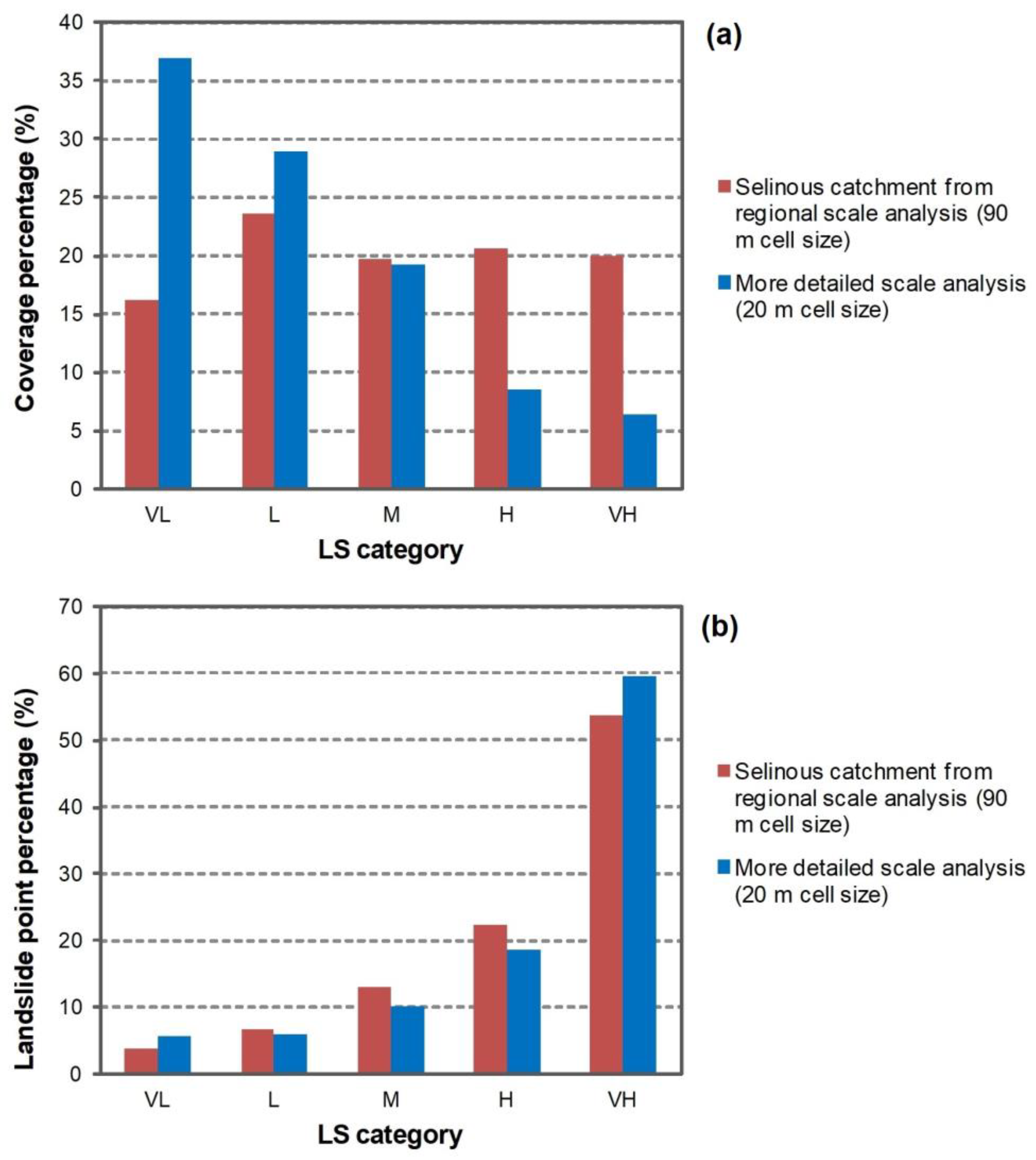
The two different scale LS maps derived from LR model are presented in Figure 3. In the regional scale LS map, “High” and “Very High” susceptibility categories are mainly located in the central and western mountainous areas of the system of catchments, including large parts across Selinous catchment (Figure 3a). According to the results of regional scale analysis for the extent of Selinous catchment, 20.6% and 19.9%, respectively, of the region (defined from the black boundary line in the Figure 3a) are covered by the two susceptibility categories (Figure 4a). Regarding the more detailed scale LS map, the corresponding susceptibility categories are concentrated in a limited area of central part of Selinous catchment (Figure 3b). Their coverage percentages in the region are 8.5% and 6.4%, respectively (Figure 4a).
To enable the comparability between the results of the two different analysis scales, their produced LS maps were cross-compared to the extent of Selinous catchment (Table 4). In terms of coverage similarities and differences between the susceptibility categories, this cross-comparison indicated that 1.8% and 2.9% of the Selinous catchment are categorized as “High” and “Very High”, respectively, susceptibility in both maps. The percentages of coverage similarities are higher for the “Very Low” and “Low” susceptibility categories (7.5% and 7.3%, respectively). Considering the coverage differences, 1.8% of the Selinous catchment is categorized as “High” susceptibility in the regional scale map, but as “Very High” susceptibility in the more detailed scale map. Furthermore, 2.2% of the catchment is characterized as “Very High” susceptibility in the regional scale map, but as “High” susceptibility in the more detailed scale map. The highest difference percentage (equal to 9.2%) is shown between the “Low” susceptibility category of the regional scale map, and the “Very Low” susceptibility category of the more detailed scale map.
The overlay of LS maps with the relative landslide datasets indicated that, for both analyses, the percentage of the landslide points is gradually increased from “Very Low” to “Very High” susceptibility categories (Figure 4b). Specifically, based on the outputs of regional scale analysis for the extent of Selinous catchment, 22.4% and 53.9% (total of 76.3%) of the landslide points occurred in the region (the landslide points within the black boundary line in Figure 1a) fall within “High” and “Very High”, respectively, susceptibility categories. From these percentages, 4% and 10%, respectively, refer to Selinous catchment. On the other hand, for the more detailed scale analysis, 18.5% and 59.7% (total of 78.2%) of the landslide points (derived from the landslide polygons in Figure 1b) in Selinous catchment fall within the same susceptibility categories.
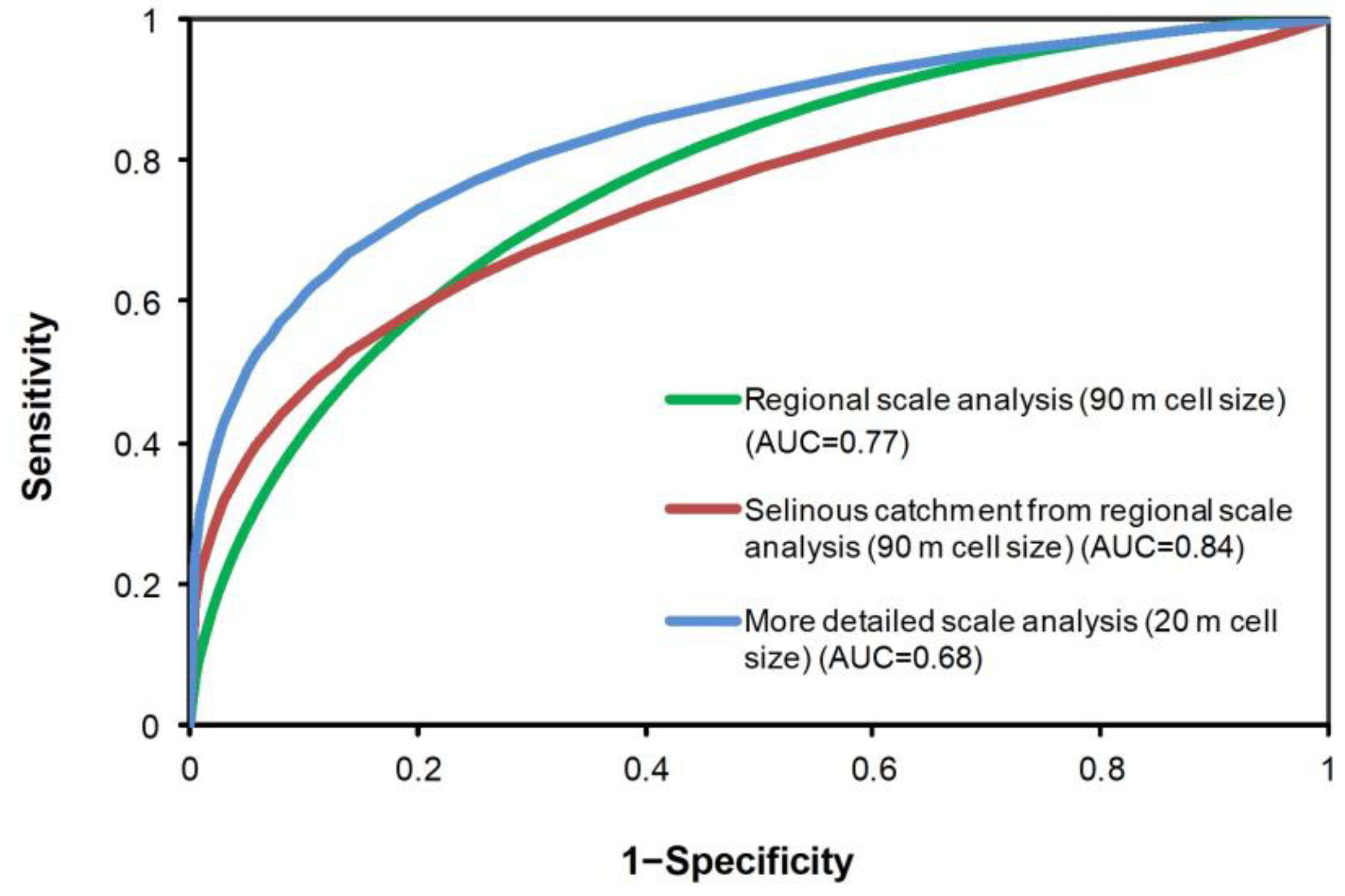
For the validation of the models, the validation datasets were matched with the categories of the two LS maps. Then, the ROC curves were drawn (Figure 5) and the various statistics were calculated (Table 5). The AUC value equal to 0.77 from the regional scale analysis indicates a good prediction ability of LR model for the entire area of the system of catchments. From the same scale analysis, this value is slightly lower (AUC = 0.74) focusing on the extent of Selinous catchment. On the contrary, the LR model is found to have very good prediction ability (AUC = 0.84) for the Selinous catchment at the more detailed scale.
6. Discussion
In the last decade, main aspiration of landslide research works is to solve deficiencies and difficulties in LS assessment in order to prepare reliable maps with as high as possible accuracy. In this study, by applying a multivariate statistical model like LR, the relationship between landslide occurrence and several causal factors was assessed and mapped at two different scales (a regional and a more detailed scale). Two landslide inventories were created using different manners for the representation of landslide occurrence. The causal factors of elevation, slope angle, profile curvature, distance to roads, stream density, geology, and NDVI were obtained as grids of different cell size (90 m and 20 m, respectively).
LR model employs the use of a set of predictor variables to create a mathematical model that predicts the probability of phenomenon occurrence in a certain area. Due to its flexible, non-linear and non-parametric nature, this model has the advantage of being able to deal with a wide range of data, and analyze variables that are non-symmetrical and show skewed distributions, typical in the natural environment [54]. On the other hand, the performance of LR depends on the quality of the data collected, and the correct identification of the causal factors in a given scale. Therefore, the analysis scale has a substantial influence on the results of the model. If the analysis is based on small-scale datasets, its results are not typically suitable for more detail-oriented scales. In contrast, more exhaustive datasets, often not available, are required at the more detailed scale analysis.
Firstly, the coefficients assigned to causal factors from LR model are useful to assess the importance of factors on the presence or absence of landslides (Table 3). In the current study, the findings from the two LS analyses are completely different. Specifically, two of the factors (distance to roads and NDVI) with the highest importance on landsliding at the regional scale analysis belong to the factors with the lowest importance at the more detailed scale analysis. Reversely, the most important factor (elevation) at the more detailed scale analysis is characterized as the least important factor at the regional scale analysis. However, the findings from the more detailed scale analysis seem to agree with the findings of the majority of LS assessment studies using LR which indicate elevation and slope angle as the most important predictor variables for estimating the probability of landslide occurrence [18].
For each of the two analyses, the outputs of LR model were used to represent the spatial distribution of the estimated LS (Figure 3). Focusing on the extent of Selinous catchment, the coverage areas of “High” and “Very High” susceptibility categories from the regional scale analysis are found to be significantly larger than these from the more detailed scale analysis (it is also confirmed from the relative percentages in Figure 4a). Focusing on the extent of Selinous catchment, it can be mentioned that as a result of these immensely high coverage areas, as well as the high sensitivity and low specificity values (Table 5), the regional scale analysis shows an overestimation of LS.
With regards to the outputs of ROC analysis, it must firstly be noted that the regional scale analysis for the entire system of catchments gives rather satisfactory results in terms of accuracy and prediction ability (Table 5). These results corroborate previous findings indicating that the coarser grids can be adequate for LS assessment, as the relationships between the size of grid cells and the predictive performance of a model depend on various factors, including the selected study area and the quality of the source data [23].
Despite this, the optimal resolution for LS assessment must be evaluated case by case. In the present study, it is accomplished by the comparison of results of the two analyses for the extent of Selinous catchment. Based on the extracted accuracy and AUC values (Table 5), the more detailed scale analysis shows much higher accuracy and prediction ability than the regional scale analysis. Thus, the high spatial resolution (smaller grid cells) of the input datasets at the more detailed scale analysis provides more reliable information about the landslide-prone parts of Selinous catchment. This finding confirms the fact that the optimization of the resolution for LS assessment depends on the size of the study area [25]. By diminishing the size of grid cells as it was required from the diminution of the size of study area, higher landslide susceptibility mapping accuracy was achieved.
Some assumptions and limitations of the two analyses and the data used in them have to be pointed out. Although the point data in GIS environment are described by individual features of spatial coordinates and do not reflect the landslide affected area, they are recommended to be used when the landslide areas cannot be drawn as polygons due to the scale of the map. On the other hand, for the polygon data, although some studies represent as polygon only the depletion zone of the landslides [55,56], the non-possibility of differentiation between this zone and accumulation zone, as well as the fact that the majority of the mapped landslides are shallow failures with small extent and limited transport length resulted to the assumption of the existence of similar conditions in terms of causal factors for these two zones and consequently to the representation as polygon of the total area for each landslide. During the sampling for the creation of dependent variable, considerable simplification of the landslide data had to be undertaken by defining a centroid point for each landslide cell. In this way, areas identified as landslide points were underestimated in some instances. Furthermore, the process for obtaining the training and validation datasets affects both the performance of the model and the accuracy of its results. It is expected that the training dataset includes a sufficient amount of data belonging to the problem domain. In contrast, the data used in the validation dataset should be distinct from the training data. Since there is no rule of thumb for determining the appropriate size of the datasets, its selection is a subjective affair. The selected number and type of causal factors, as well as their classification also contribute to the accuracy of the results. The examination of alternative choices for these parameters could lead to different findings. Moreover, the applied model of LR estimates the mean degree of impact of causal factors, which may differ locally in different parts of the area under investigation. In fact, it represents the relation between landslide occurrence and causal factors for the entire area without considering the spatial non-stationarity in this relation. Finally, it should be noted that the produced LS maps illustrate only the predicted spatial probability, and not the temporal probability of landslides.
7. Conclusions
Based on the fact that the scale of analysis has considerable influence on the performance of a LS model, hazardous landslide areas were mapped using the outputs of LR model at two different scales. The results revealed that the LS assessment can be substantially affected by the scale of analysis. Furthermore, the spatial resolution constitutes a key factor on the accuracy of LS assessment and the optimal size of grid cells depends on the size of the study area. The promising results of the regional scale analysis indicate that it can be safely used for large regions with limited availability of detailed data. However, focusing on the Selinous catchment, the confirmed with higher accuracy and reliability LS map derived from the more detailed scale analysis could constitute an essential base in the primary stage of landslide risk management and mitigation for the region. Specifically, the produced map could aid the local authorities, decision makers and planners to identify land uses and infrastructures subject to damage by future landslides and choose suitable locations for the implementation of developments.
Author Contributions
Conceptualization, C.C., C.P. and A.F.; Methodology, C.P., A.F. and C.C.; Validation, C.P. and A.F.; Writing-Original Draft Preparation, C.P., A.F. and C.C.; Visualization, A.F. and C.P.
Funding
This research was funded by the Hellenic Foundation for Research and Innovation (HFRI) of the General Secretariat for Research and Technology (GSRT).
Acknowledgments
The authors are grateful to the anonymous reviewers for their valuable comments and constructive manuscript revision.
Conflicts of Interest
The authors declare no conflict of interest.
References
- Highland, L.M.; Bobrowsky, P. The Landslide Handbook—A Guide to Understanding Landslides; U.S. Geological Survey Circular 1325; U.S. Geological Survey: Reston, VA, USA, 2008; p. 129.
- Centre for Research on the Epidemiology of Disasters (CRED). 2016 Preliminary Data1: Human Impact of Natural Disasters2; CRED CRUNCH 2016, No. 45; Centre for Research on the Epidemiology of Disasters (CRED): Brussels, Belgium, 2016; p. 2. Available online: https://www.cred.be/downloadFile.php?file=sites/default/files/CredCrunch45.pdf (accessed on 22 May 2018).
- Centre for Research on the Epidemiology of Disasters (CRED). Disaster Data: A Balanced Perspective; CRED CRUNCH 2017, No. 48; Centre for Research on the Epidemiology of Disasters (CRED): Brussels, Belgium, 2017; p. 2. Available online: https://www.cred.be/downloadFile.php?file=sites/default/files/CredCrunch48.pdf (accessed on 22 May 2018).
- Koukis, G.; Sabatakakis, N.; Nikolaou, N.; Loupasakis, C. Landslide hazard zonation in Greece. In Landslides: Risk Analysis and Sustainable Disaster Management; Sassa, K., Fukuoka, H., Wang, F., Wang, G., Eds.; Springer: Berlin, Germany, 2005; pp. 291–296. [Google Scholar]
- Parcharidis, I.; Vassilakis, E.; Cooksley, G.; Metaxas, C. Sesmically-triggered landslide risk, assessment. In Earthquake Geodynamics: Seismic Case Studies, Series: Advances in Earthquake Engineering; Lekkas, E., Ed.; WIT Press: Southampton, UK, 2004; pp. 119–127. [Google Scholar]
- Sabatakakis, N.; Koukis, G.; Vassiliades, E.; Lainas, S. Landslide susceptibility zonation in Greece. Nat. Hazards 2013, 65, 523–543. [Google Scholar] [CrossRef]
- Van Westen, C.J.; Van Asch, T.W.J.; Soeters, R. Landslide hazard and risk zonation—Why is it still so difficult? Bull. Eng. Geol. Environ. 2006, 65, 167–184. [Google Scholar] [CrossRef]
- Corominas, J.; Van Westen, C.; Frattini, P.; Cascini, L.; Malet, J.P.; Fotopoulou, S.; Catani, F.; Van Den Eeckhaut, M.; Mavrouli, O.; Agliardi, F.; et al. Recommendations for the quantitative analysis of landslide risk. Bull. Eng. Geol. Environ. 2014, 73, 209–263. [Google Scholar] [CrossRef] [Green Version]
- Reichenbach, P.; Rossi, M.; Malamud, B.; Mihir, M.; Guzzetti, F. A review of statistically-based landslide susceptibility models. Earth-Sci. Rev. 2018, 180, 60–91. [Google Scholar] [CrossRef]
- Mansouri Daneshvar, M.R. Landslide susceptibility zonation using analytical hierarchy process and GIS for the Bojnurd region, northeast of Iran. Landslides 2014, 11, 1079–1091. [Google Scholar] [CrossRef]
- Chen, X.; Chen, H.; You, Y.; Liu, J. Susceptibility assessment of debris flows using the analytic hierarchy process method—A case study in Subao river valley, China. J. Rock Mech. Geotech. Eng. 2015, 7, 404–410. [Google Scholar] [CrossRef]
- Dahal, R.K.; Bhandary, N.P.; Hasegawa, S.; Yatabe, R. Topo-stress based probabilistic model for shallow landslide susceptibility zonation in the Nepal Himalaya. Environ. Earth Sci. 2014, 71, 3879–3892. [Google Scholar] [CrossRef]
- Pradhan, A.M.S.; Kim, Y.-T. Application and comparison of shallow landslide susceptibility models in weathered granite soil under extreme rainfall events. Environ. Earth Sci. 2015, 73, 5761–5771. [Google Scholar] [CrossRef]
- Carrara, A. Multivariate models for landslide hazard evaluation. Math. Geol. 1983, 15, 403–426. [Google Scholar] [CrossRef]
- Carrara, A.; Cardinali, M.; Detti, R.; Guzzetti, F.; Pasqui, V.; Reichenbach, P. GIS techniques and statistical models in evaluating landslide hazard. Earth Surf. Processes Landf. 1991, 16, 427–445. [Google Scholar] [CrossRef]
- Chung, C.J.F.; Fabbri, A.G.; Van Westen, C.J. Multivariate regression analysis for landslide hazard zonation. In Geographical Information Systems in Assessing Natural Hazards; Carrara, A., Guzzetti, F., Eds.; Kluwer Pub.: Dordrecht, The Netherlands, 1995; pp. 107–133. [Google Scholar]
- Lee, S.; Min, K. Statistical analysis of landslide susceptibility at Yongin, Korea. Environ. Geol. 2001, 40, 1095–1113. [Google Scholar] [CrossRef]
- Ayalew, L.; Yamagishi, H. The application of GIS-based logistic regression for landslide susceptibility mapping in the Kakuda-Yahiko Mountains Central Japan. Geomorphology 2005, 65, 15–31. [Google Scholar] [CrossRef]
- Sdao, F.; Lioi, D.S.; Pascale, S.; Caniani, D.; Mancini, I.M. Landslide susceptibility assessment by using a neuro-fuzzy model: A case study in the Rupestrian heritage rich area of Matera. Nat. Hazards Earth Syst. Sci. 2013, 13, 395–407. [Google Scholar] [CrossRef]
- Park, I.; Lee, S. Spatial prediction of landslide susceptibility using a decision tree approach: A case study of the Pyeongchang area, Korea. Int. J. Remote Sens. 2014, 35, 6089–6112. [Google Scholar] [CrossRef]
- Su, C.; Wang, L.; Wang, X.; Huang, Z.; Zhang, X. Mapping of rainfall-induced landslide susceptibility in Wencheng, China, using support vector machine. Nat. Hazards 2015, 76, 1759–1779. [Google Scholar] [CrossRef]
- Gorsevski, P.V.; Brown, M.K.; Panter, K.; Onasch, C.M.; Simic, A.; Snyder, J. Landslide detection and susceptibility mapping using LiDAR and an artificial neural network approach: A case study in the Cuyahoga Valley National Park, Ohio. Landslides 2016, 13, 467–484. [Google Scholar] [CrossRef]
- Cama, M.; Conoscenti, C.; Lombardo, L.; Rotigliano, E. Exploring relationships between grid cell size and accuracy for debris-flow susceptibility models: A test in the Giampilieri catchment (Sicily, Italy). Environ. Earth Sci. 2016, 75, 238. [Google Scholar] [CrossRef]
- Lee, S.; Choi, J.; Woo, I. The effect of spatial resolution on the accuracy of landslide susceptibility mapping: A case study in Boun, Korea. Geosci. J. 2004, 8, 51. [Google Scholar] [CrossRef]
- Tian, Y.; Xiao, C.; Liu, Y.; Wu, L. Effects of raster resolution on landslide susceptibility mapping: A case study of Shenzhen. Sci. China Ser. E Technol. Sci. 2008, 51, 188–198. [Google Scholar] [CrossRef]
- Palamakumbure, D.; Flentje, P.; Stirling, D. Consideration of optimal pixel resolution in deriving landslide susceptibility zoning within the Sydney Basin, New South Wales, Australia. Comput. Geosci. 2015, 82, 13–22. [Google Scholar] [CrossRef]
- Special Secretariat for Water. Management Plan for the River Catchments of Drainage District of Northern Peloponnese; Ministry of Environment, Energy and Climate Change: Athens, Greece, 2012; p. 456. [Google Scholar]
- Pnevmatikos, J.D.; Katsoulis, B.D. The changing rainfall regime in Greece and its impact on climatological means. Meteorol. Appl. 2006, 13, 331–345. [Google Scholar] [CrossRef]
- Sabatakakis, N.; Koukis, G.; Mourtas, D. Composite landslides induced by heavy rainfalls in suburban areas: City of Patras and surrounding area, western Greece. Landslides 2005, 2, 202–211. [Google Scholar] [CrossRef]
- Wieczorek, G.F. Preparing a detailed landslide-inventory map for hazard evaluation and reduction. Bull. Assoc. Eng. Geol. 1984, 21, 337–342. [Google Scholar] [CrossRef]
- Guzzetti, F.; Mondini, A.C.; Cardinali, M.; Fiorucci, F.; Santangelo, M.; Chang, K.T. Landslide inventory maps: New tools for an old problem. Earth-Sci. Rev. 2012, 112, 42–66. [Google Scholar] [CrossRef]
- Tsagas, D. Geomorphological Investigation and Mass Movements in Northern Peloponnese: Area of Xylokastro-Diakofto. Ph.D. Thesis, National and Kapodistrian University of Athens, Zografou, Greece, 2011. [Google Scholar]
- Laboratory of Engineering Geology, Department of Geology, University of Patras, Landslide Inventory Database. Available online: http://www.geoarch.gr/ (accessed on 5 September 2016).
- Cruden, D.M.; Varnes, D.J. Landslide types and processes. In Landslides: Investigation and Mitigation; Special Report 247; Turner, A.K., Schuster, R.L., Eds.; Transportation Research Board, National Research Council: Washington, DC, USA, 1996; pp. 36–75. [Google Scholar]
- Clerici, A.; Perego, S.; Tellini, C.; Vescovi, P. A GIS-based automated procedure for landslide susceptibility mapping by the Conditional Analysis method: The Baganza valley case study (Italian Northern Apennines). Environ. Geol. 2006, 50, 941–961. [Google Scholar] [CrossRef]
- Van Westen, C.J.; Castellanos, E.; Kuriakose, S.L. Spatial data for landslide susceptibility, hazard, and vulnerability assessment: An overview. Eng. Geol. 2008, 102, 112–131. [Google Scholar] [CrossRef]
- Pradhan, A.M.S.; Kim, Y.-T. Relative effect method of landslide susceptibility zonation in weathered granite soil: A case study in Deokjeok-ri Creek, South Korea. Nat. Hazards 2014, 72, 1189–1217. [Google Scholar] [CrossRef]
- Youssef, A.M. Landslide susceptibility delineation in the Ar-Rayth area, Jizan, Kingdom of Saudi Arabia, using analytical hierarchy process, frequency ratio, and logistic regression models. Environ. Earth Sci. 2015, 73, 8499–8518. [Google Scholar] [CrossRef]
- Meng, Q.; Miao, F.; Zhen, J.; Wang, X.; Wang, A.; Peng, Y.; Fan, Q. GIS-based landslide susceptibility mapping with logistic regression, analytical hierarchy process, and combined fuzzy and support vector machine methods: A case study from Wolong Giant Panda Natural Reserve, China. Bull. Eng. Geol. Environ. 2016, 75, 923–944. [Google Scholar] [CrossRef]
- Dai, F.C.; Lee, C.F. Landslide characteristics and slope instability modeling using GIS, Lantau Island, Hong Kong. Geomorphology 2002, 42, 213–228. [Google Scholar] [CrossRef]
- Saito, H.; Nakayama, D.; Matsuyama, H. Comparison of landslide susceptibility based on a decision-tree model and actual landslide occurrence: the Akaishi Mountains, Japan. Geomorphology 2009, 109, 108–121. [Google Scholar] [CrossRef]
- Shahabi, H.; Hashim, M. Landslide susceptibility mapping using GIS-based statistical models and remote sensing data in tropical environment. Sci. Rep. 2015, 5, 9899. [Google Scholar] [CrossRef] [PubMed]
- Intarawichian, N.; Dasananda, S. Frequency ratio model based landslide susceptibility mapping in lower Mae Chaem watershed, Northern Thailand. Environ. Earth Sci. 2011, 64, 2271–2285. [Google Scholar] [CrossRef]
- Atkinson, P.M.; Massari, R. Generalized linear modeling of susceptibility to landsliding in the central Apennines, Italy. Comput. Geosci. 1998, 24, 373–385. [Google Scholar] [CrossRef]
- Hosmer, D.W.; Lemeshow, S. Applied Logistic Regression; Wiley: New York, NY, USA, 1989; p. 328. [Google Scholar]
- Kundu, S.; Saha, A.K.; Sharma, D.C.; Pant, C.C. Remote Sensing and GIS Based Landslide Susceptibility Assessment using Binary Logistic Regression Model: A Case Study in the Ganeshganga Watershed, Himalayas. J. Indian Soc. Remote Sens. 2013, 41, 697–709. [Google Scholar] [CrossRef]
- Raja, N.B.; Çiçek, I.; Türkoğlu, N.; Aydin, O.; Kawasaki, A. Landslide susceptibility mapping of the Sera River Basin using logistic regression model. Nat. Hazards 2017, 85, 1323–1346. [Google Scholar] [CrossRef]
- Jenks, G.F. Optimal Data Classification for Choropleth Maps; Occasional Paper No. 2; Department of Geographv, University of Kansas: Lawrence, KS, USA, 1977. [Google Scholar]
- Bai, S.B.; Wang, J.; Lü, G.N.; Zhou, P.G.; Hou, S.S.; Xu, S.N. GIS-based logistic regression for landslide susceptibility mapping of the Zhongxian segment in the Three Gorges area, China. Geomorphology 2010, 115, 23–31. [Google Scholar] [CrossRef]
- Gorsevski, P.V.; Gessler, P.E.; Foltz, R.B.; Elliot, W.J. Spatial prediction of landslide hazard using logistic regression and ROC analysis. Trans. GIS 2006, 10, 395–415. [Google Scholar] [CrossRef]
- Frattini, P.; Crosta, G.; Carrara, A. Techniques for evaluating the performance of landslide susceptibility models. Eng. Geol. 2010, 111, 62–72. [Google Scholar] [CrossRef]
- Althuwaynee, O.F.; Pradhan, B.; Park, H.J.; Lee, J.H. A novel ensemble decision tree-based CHi-squared Automatic Interaction Detection (CHAID) and multivariate logistic regression models in landslide susceptibility mapping. Landslides 2014, 11, 1063–1078. [Google Scholar] [CrossRef]
- Cervi, F.; Berti, M.; Borgatti, L.; Ronchetti, F.; Manenti, F.; Corsini, A. Comparing predictive capability of statistical and deterministic methods for landslide susceptibility mapping: a case study in the northern Apennines (Reggio Emilia Province, Italy). Landslides 2010, 7, 433–444. [Google Scholar] [CrossRef]
- Nandi, A.; Shakoor, A. A GIS-based landslide susceptibility evaluation using bivariate and multivariate statistical analyses. Eng. Geol. 2009, 110, 11–20. [Google Scholar] [CrossRef]
- Othman, A.A.; Gloaguen, R.; Andreani, L.; Rahnama, M. Landslide susceptibility mapping in Mawat area, Kurdistan Region, NE Iraq: a comparison of different statistical models. Nat. Hazards Earth Syst. Sci. Discuss. 2015, 3, 1789–1833. [Google Scholar] [CrossRef]
- Van Den Eeckhaut, M.; Vanwalleghem, T.; Poesen, J.; Govers, G.; Verstraeten, G.; Vandekerckhove, L. Prediction of landslide susceptibility using rare events logistic regression: A case-study in the Flemish Ardennes (Belgium). Geomorphology 2006, 76, 392–410. [Google Scholar] [CrossRef]
Figure 1.
The landslide inventory map (a) of systems of catchments for the regional scale analysis, including the location map (b) of Selinous catchment for the more detailed scale analysis.
Figure 1.
The landslide inventory map (a) of systems of catchments for the regional scale analysis, including the location map (b) of Selinous catchment for the more detailed scale analysis.

Figure 2.
Causal factors: (a) Elevation; (b) slope angle; (c) profile curvature; (d) distance to roads; (e) stream density; (f) NDVI; (g) geology.
Figure 2.
Causal factors: (a) Elevation; (b) slope angle; (c) profile curvature; (d) distance to roads; (e) stream density; (f) NDVI; (g) geology.

Figure 3.
The landslide susceptibility maps produced by the model (a) for the regional scale analysis; (b) for the more detailed scale analysis.
Figure 3.
The landslide susceptibility maps produced by the model (a) for the regional scale analysis; (b) for the more detailed scale analysis.

Figure 4.
Diagrams with: (a) The coverage area percentages; and (b) the percentages of landslide points for landslide susceptibility categories (VL: Very Low, L: Low, M: Moderate, H: High, VH: Very High) derived from the two analyses focusing on the extent of Selinous catchment.
Figure 4.
Diagrams with: (a) The coverage area percentages; and (b) the percentages of landslide points for landslide susceptibility categories (VL: Very Low, L: Low, M: Moderate, H: High, VH: Very High) derived from the two analyses focusing on the extent of Selinous catchment.

Figure 5.
Receiver operating characteristics (ROC) curves of the LR model for the regional scale analysis (referring to both the entire system of catchments and Selinous catchment) and the more detailed scale analysis.
Figure 5.
Receiver operating characteristics (ROC) curves of the LR model for the regional scale analysis (referring to both the entire system of catchments and Selinous catchment) and the more detailed scale analysis.


Table 1.
Geographic Information Systems (GIS) Layers of the datasets representing the causal factors.
Table 1.
Geographic Information Systems (GIS) Layers of the datasets representing the causal factors.
| Type | Factors | Primary Data | Format | |
|---|---|---|---|---|
| Regional Scale Analysis (90 m Cell Size) | More Detailed Scale Analysis (20 m Cell Size) | |||
| Topography | Elevation | SRTM dataset | Vector layers of 5 m contours and elevation points | Grid |
| Slope angle | Derived from SRTM DEM | Derived from vector-based DEM | Grid | |
| Profile curvature | Derived from SRTM DEM | Derived from vector-based DEM | Grid | |
| Hydrology | Stream density | Vector layer of drainage network (General Use Map of Greece 1:250,000 by Hellenic Military Geographical Service) | Vector layer of drainage network (General Use Map of Greece 1:50,000 by Hellenic Military Geographical Service) | Grid |
| Road proximity | Distance to roads | Vector layer of main road network (OpenStreetMap) | Vector layer of road network (OpenStreetMap) | Grid |
| Geology | Geology | Generalized geological formations (Geological Map of Greece 1:50,000 by Institute of Geology and Mineral Exploration) | Detailed geological formations (Geological Map of Greece 1:50,000 by Institute of Geology and Mineral Exploration) | Vector (polygons) |
| Vegetation | NDVI | Landsat-8 images (30 m spatial resolution, taken in February 2016) | Sentinel-2 images (10 m spatial resolution, taken in April 2017) | Grid |
Table 2.
Multicollinearity checking indexes for the causal factors.
| Causal Factors | Regional Scale Analysis (90 m Cell Size) | More Detailed Scale Analysis (20 m Cell Size) | ||
|---|---|---|---|---|
| TOL | VIF | TOL | VIF | |
| Elevation | 0.908 | 1.101 | 0.933 | 1.072 |
| Slope angle | 0.891 | 1.122 | 0.748 | 1.337 |
| Profile curvature | 0.969 | 1.032 | 0.998 | 1.002 |
| Stream density | 0.930 | 1.076 | 0.936 | 1.068 |
| Distance to roads | 0.914 | 1.094 | 0.675 | 1.482 |
| Geology | 0.930 | 1.075 | 0.757 | 1.321 |
| NDVI | 0.940 | 1.063 | 0.904 | 1.106 |
Table 3.
Coefficients derived from logistic regression (LR) model for the causal factors.
| Causal Factors | Coefficients | |
|---|---|---|
| Regional Scale Analysis (90 m Cell Size) | More Detailed Scale Analysis (20 m Cell Size) | |
| Elevation | 2.007 | 9.178 |
| Slope angle | 5.664 | 4.474 |
| Profile curvature | 2.505 | 3.056 |
| Stream density | 4.027 | 4.796 |
| Distance to roads | 6.227 | 2.258 |
| Geology | 8.019 | 3.475 |
| NDVI | 6.856 | 2.880 |
| (Constant) | (−8.333) | (−7.309) |
Table 4.
Coverage percentage (%)-based cross-comparisons for the landslide susceptibility (LS) categories between the Selinous catchment from the regional scale analysis and more detailed scale analysis.
Table 4.
Coverage percentage (%)-based cross-comparisons for the landslide susceptibility (LS) categories between the Selinous catchment from the regional scale analysis and more detailed scale analysis.
| Selinous Catchment from Regional Scale Analysis (90 m Cell Size) | More Detailed Scale Analysis (20 m Cell Size) | ||||
|---|---|---|---|---|---|
| VL | L | M | H | VH | |
| VL | 7.5 | 4.4 | 3.0 | 1.0 | 0.2 |
| L | 9.2 | 7.3 | 4.6 | 1.8 | 0.7 |
| M | 7.1 | 5.9 | 3.8 | 1.7 | 1.0 |
| H | 7.2 | 6.0 | 3.9 | 1.8 | 1.8 |
| VH | 5.9 | 5.2 | 3.9 | 2.2 | 2.9 |
Table 5.
ROC analysis results of the LR model for the regional scale analysis (referring both the entire system of catchments and Selinous catchment) and the more detailed scale analysis.
Table 5.
ROC analysis results of the LR model for the regional scale analysis (referring both the entire system of catchments and Selinous catchment) and the more detailed scale analysis.
| ROC Analysis Results | Regional Scale Analysis (90 m Cell Size) | Selinous Catchment from Regional Scale Analysis (90 m Cell Size) | More Detailed Scale Analysis (20 m Cell Size) |
|---|---|---|---|
| Number of cases | 164 | 31 | 892 |
| Number correct | 115 | 24 | 679 |
| Positive cases missed | 17 | 4 | 72 |
| Negative cases missed | 32 | 3 | 141 |
| Accuracy (%) | 70.1 | 69.6 | 76.1 |
| Sensitivity (%) | 79.3 | 82.6 | 83.9 |
| Specificity (%) | 61.0 | 62.5 | 68.4 |
| AUC value | 0.77 | 0.74 | 0.84 |
© 2018 by the authors. Licensee MDPI, Basel, Switzerland. This article is an open access article distributed under the terms and conditions of the Creative Commons Attribution (CC BY) license (http://creativecommons.org/licenses/by/4.0/).
Share and Cite
MDPI and ACS Style
Polykretis, C.; Faka, A.; Chalkias, C. Exploring the Impact of Analysis Scale on Landslide Susceptibility Modeling: Empirical Assessment in Northern Peloponnese, Greece. Geosciences 2018, 8, 261. https://doi.org/10.3390/geosciences8070261
AMA Style
Polykretis C, Faka A, Chalkias C. Exploring the Impact of Analysis Scale on Landslide Susceptibility Modeling: Empirical Assessment in Northern Peloponnese, Greece. Geosciences. 2018; 8(7):261. https://doi.org/10.3390/geosciences8070261
Chicago/Turabian StylePolykretis, Christos, Antigoni Faka, and Christos Chalkias. 2018. "Exploring the Impact of Analysis Scale on Landslide Susceptibility Modeling: Empirical Assessment in Northern Peloponnese, Greece" Geosciences 8, no. 7: 261. https://doi.org/10.3390/geosciences8070261
Note that from the first issue of 2016, this journal uses article numbers instead of page numbers. See further details here.