Re-Aeration on Stepped Spillways with Special Consideration of Entrained and Entrapped Air


1
Hydraulic Engineering Section (HES), FH Aachen University of Applied Sciences, Bayernallee 9, 52066 Aachen, Germany
2
Department of ArGEnCo, Research Group of Hydraulics in Environmental and Civil Engineering (HECE), University of Liege (ULg), 4000 Liège, Belgium
*
Author to whom correspondence should be addressed.
Geosciences 2018, 8(9), 333; https://doi.org/10.3390/geosciences8090333
Submission received: 4 August 2018
/
Revised: 28 August 2018
/
Accepted: 3 September 2018
/
Published: 5 September 2018
(This article belongs to the Special Issue Beyond the Channel—Investigating Processes at Crucial Fluvial Interfaces)
Abstract
:As with most high-velocity free-surface flows, stepped spillway flows become self-aerated when the drop height exceeds a critical value. Due to the step-induced macro-roughness, the flow field becomes more turbulent than on a similar smooth-invert chute. For this reason, cascades are oftentimes used as re-aeration structures in wastewater treatment. However, for stepped spillways as flood release structures downstream of deoxygenated reservoirs, gas transfer is also of crucial significance to meet ecological requirements. Prediction of mass transfer velocities becomes challenging, as the flow regime differs from typical previously studied flow conditions. In this paper, detailed air-water flow measurements are conducted on stepped spillway models with different geometry, with the aim to estimate the specific air-water interface. Re-aeration performances are determined by applying the absorption method. In contrast to earlier studies, the aerated water body is considered a continuous mixture up to a level where 75% air concentration is reached. Above this level, a homogenous surface wave field is considered, which is found to significantly affect the total air-water interface available for mass transfer. Geometrical characteristics of these surface waves are obtained from high-speed camera investigations. The results show that both the mean air concentration and the mean flow velocity have influence on the mass transfer. Finally, an empirical relationship for the mass transfer on stepped spillway models is proposed.
1. Introduction
Stepped spillways and cascades are known to be effective energy dissipaters downstream of reservoirs due to the increased flow resistance created by the steps [1]. In addition, the step-induced macro-roughness leads to higher turbulence compared to smooth-invert chutes, which in turn significantly affects the flow structure. Similar to smooth-invert spillways, stepped spillway flows become self-aerated depending on the discharge, slope and spillway extension [1,2,3]. Once the self-aeration has been triggered, the water surface becomes more and more disturbed, and bubbles, entrained in water, as well as droplets, ejected to the air, are transported along the chute. This involves a significant specific air-water interface across which gas transfer can take place. In particular, oxygen transfer is of high interest as water in reservoirs often suffer from deoxygenation, there being a level of dissolved oxygen (DO) content required to keep good ecological conditions in downstream rivers and streams.
Chanson [4] stated that the re-aeration potential of stepped spillways is higher than for smooth-invert chutes with an identical slope. Moreover, the re-aeration in a skimming flow regime (i.e. a flow regime where water flows down the chute as a coherent stream over the pseudo-bottom formed by the step edges) becomes higher for lower discharges. Several studies have been conducted in the past to describe this re-aeration potential E, which relates the oxygen deficit upstream of the structure to the remaining deficit at the downstream end, as functions of the structure’s geometry [5,6,7,8,9,10,11,12].
However, all of these studies only focus on the global aeration performance and do not investigate the gas transfer mechanism itself. In order to physically describe the gas transfer process, knowledge of the specific air-water interface and a feasible gas transfer model are essential. The latter typically depends on flow conditions, for example, mean air concentration, velocity and turbulence, and needs to be estimated by means of experiments.
In this paper, the gas transfer velocity is determined for stepped spillway flows by conducting detailed measurements of the air-water flow properties and time series of dissolved oxygen content. In contrary to earlier studies, the air-water mixture is assumed to consist of a bubbly flow region (entrained air) below a wavy surface (entrapped air), following insights of [13,14,15].
2. Background
2.1. Gas Diffusion
Gas transfer between water and air is driven by an existing concentration gradient grad (Cgas) and may be described by Fick’s 1st law, according to which the diffusive flux Igas (in mg/(m2s)) is proportional to this gradient and directed from high concentrations to low concentrations:
with Dgas the diffusion coefficient (in m2/s). Dgas depends on the temperature and is a measure for gas transfer velocity. Considering mass conservation and assuming an isotropic diffusivity, a diffusion equation is found as
For the one-dimensional diffusion perpendicular to the air-water interface, Equation (2) becomes
To solve Equation (3), the diffusion length n needs to be known, which, however, depends on the viscosity and the diffusivity itself [16]. The following empirical gas transfer model becomes thus better suited for practical applications:
with CL the gas concentration in the liquid phase, CS the saturation concentration, A the interface available for gas transfer in the water volume V and k the mass transfer coefficient (in m/s). The reciprocal value of k can be considered as the resistance involved from both phases (index “L” for liquid and “G” for gas) [17]:
with HG = CG/CL the dimensionless Henry coefficient, depending on salinity, temperature and pressure. It is worth noting that kG is about 40 to 1000 larger than kL, according to [18], for water and air (depending on turbulence), and HG is approximately 32 for oxygen. The mass transfer coefficient k in Equation (4) can thus be replaced by kL of the water phase only:
with a = A/V the specific air-water interface.
2.2. Mass Transfer Coefficient
Besides some classical, conceptional approaches, such as the two-film model of Lewis & Whitman [17], the penetration model of Higbie [19] and the surface-renewal model of Danckwerts [20], more complex, hydrodynamic models were developed later, such as the Large-Eddy model of Fortescue & Pearson [21], the Small-Eddy model by Lamont & Scott [22] and the Modified-Small-Eddy model by Moog & Jirka [23], or the turbulence-based model by Gualtieri & Gualtieri [24].
The experimental studies of other researchers show a significant influence on the mean flow velocity, Reynolds number and mean air concentration [25], while others pinpointed the influence of bubble sizes [26].
It must be noted that all of these mass transfer models have been developed for specific flow conditions that hardly compare to stepped spillway flows. The chaotic flow regime in skimming flows on a stepped spillway involves significantly higher turbulence and a more intense gas exchange than, for instance, rising bubbles in vertical pipes (case for some of these models). As pointed out by Demars & Manson [27], estimation of the air-water interface in self-aerated flows becomes non-trivial due to bubbles and spray. A more detailed experimental investigation of the re-aeration on stepped spillways and derivation of a suitable mass transfer equation is necessary.
2.3. Specific Air-Water Interface
With consideration of a simple continuity concept and assumption of spherical bubbles, Chanson [28] proposed to estimate the specific air-water interface by:
Derivation of Equation (7) is based on a statistical relation between the Sauter diameter, typically measured by an air concentration probe, and the diameter of a spherical bubble. FB is the number of detected bubbles (or droplets) per unit of time (in Hz), which can be directly extracted from the phase detection probe signals, and u(z) is the streamwise flow velocity. Toombes [29] and Toombes & Chanson [30] suggested applying this approach for larger bubbles as well, despite the fact that the shape can differ from an ideal sphere.
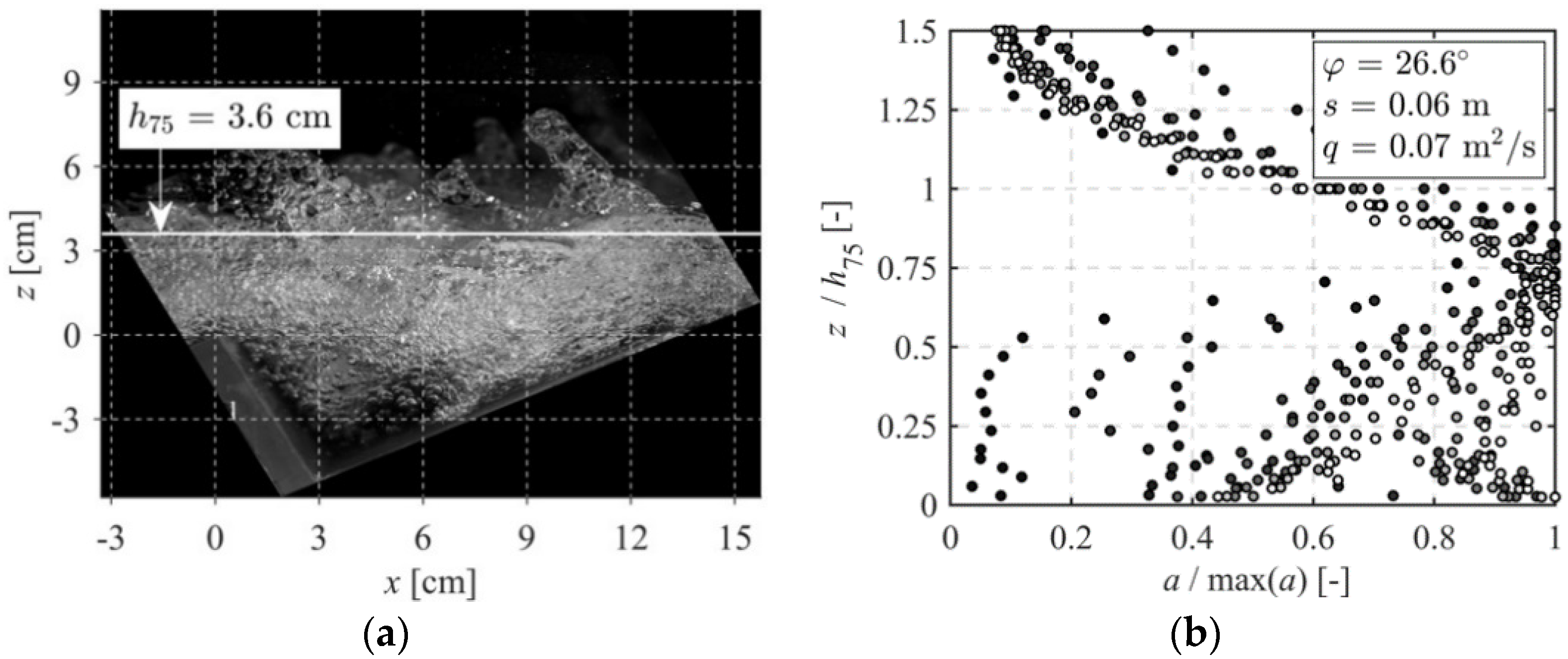
However, it is known that the air-water mixture in a stepped spillway flow may be regarded in different ways. While classical approaches assume a homogenous continuum between the bottom and h90, that is, the flow depth where the time-averaged air concentration is 90% [31,32], some recent studies distinguish a lower region with entrained air bubbles from an upper region where the air content mainly comes from air pockets being entrapped between surface waves [13,33,34,35]. Similar flow structures were reported for smooth-invert chutes [14,15]. In different studies, with different geometrical configurations, some characteristic elevations of the maximum wave trough extensions on stepped spillways are proposed. For the setup analyzed in this paper, Bung [13] suggested h75, that is, the flow depth with 75% mean air concentration, as the lower extension of the surface waves. Figure 1a shows an exemplary frame taken from a high-speed video in the quasi-uniform flow region of a model test with 1:2 slope (ϕ = 26.6°), s = 6 cm step height and a specific discharge of q = 0.07 m2/s (compare [36]). The level of h75, detected with an air concentration probe, is also indicated. It can be seen that for higher elevations, the flow structure changes and the application of Equation (7) becomes questionable for higher levels. Figure 1b shows the distribution of the dimensionless specific air-water interface a/max(a) assuming Equation (7) along the full z-coordinate up to the level corresponding to 99% air concentration. The change of the air-water flow structure for the surface wave region becomes obvious again.
3. Methodology
3.1. General Comments (Data Base)
The current paper presents a re-analysis of air-water flow data and oxygenation data published in [37,38,39,40], respectively. While these studies considered a continuous air-water mixture up to h90, the current study accounts for h75 as the upper extent of this bubbly layer. In order to account for the air-water surface roughness due to the surface waves [13], an idealized, simple sinusoidal surface is considered. Air bubbles being entrained within these surface waves are not regarded. An analytical derivation of relevant equations and necessary approximations to describe the surface geometry and its volume beneath the waves is given in Appendix A.
All data has been gathered on a physical model with slopes 1:3 and 1:2, step heights s of 3 cm and 6 cm and discharges of q = 0.07, 0.09 and 0.11 m2/s in the Hydraulics laboratory of Wuppertal University [37]. The chute width was 30 cm and its total drop height was 2.34 m. Skimming flow was found for all model tests (compare [41,42,43]). Water discharge was regulated with a flap valve, controlled with a flow meter and pumped into an open head tank before being conveyed into the spillway. The chute was part of a closed water circuit.
3.2. Air-Water Flow Measurements
Air-water flow measurements are conducted using a double-tip conductivity probe in the flume centreline. This probe consists of two needle tips with a diameter of 0.13 mm. Both tips are aligned in flow direction with a lateral spacing of 1 mm which aim to pierce up entrained bubbles and ejected droplets. By a change of resistivity depending on the surrounding medium, phase changes can be detected by applying a thresholding technique [44]. Further information on this type of probe can be found in [45]. With the assumption that (1) both tips pierce the same bubbles and (2) bubbles are transported in a slip-free way, cross-correlation of both signals yields an estimate of the flow velocity. Relevant parameters, such as the local, time-averaged air concentration, the Sauter diameter and bubble count rate can be directly determined from the signals. Additional parameters, for example, the specific air-water interface according to Equation (7), can be indirectly estimated from this data. For all configurations, tests are conducted from the inception point of self-aeration to farther downstream where quasi-uniform flow conditions set in. For the larger steps, data is gathered at step edges and above the centre of the step cavity. For the smaller steps, all data is obtained at step edges only.
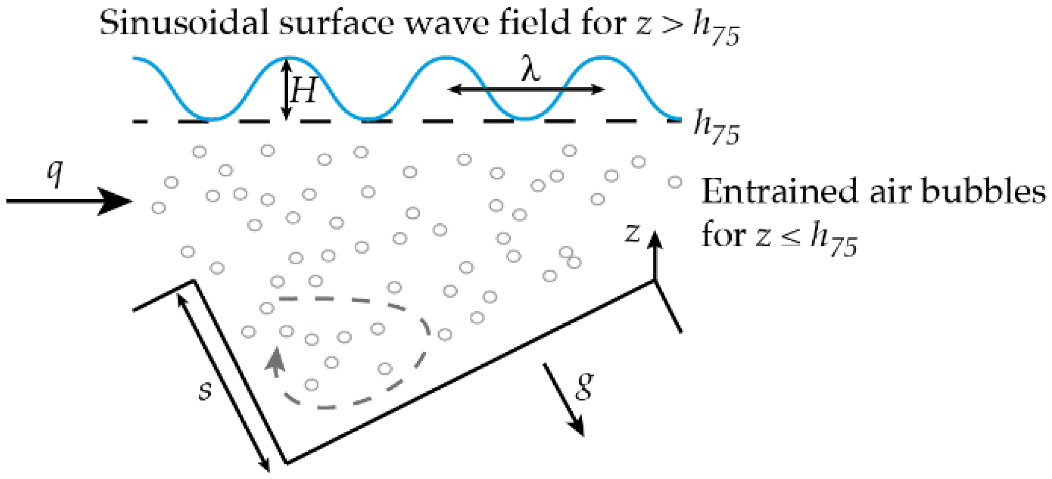
As the extraction of surface waves (Figure 1a) from conductivity probe data and the determination of the available air-water interface above h75 is not directly possible, a continuum up to h75 is considered in this study and a three-dimensional sinusoidal wave field (with waveheights H and wavelengths λ), leading to an interfacial surface of the air-water mixture. The latter is added to the interface Aent formed by the entrained air bubbles. A schematic illustration of the employed concept is shown in Figure 2. In order to determine the specific air-water interface, Atot = Aent + needs to be related to the total volume (up to the upper wave extent).
3.3. Surface Wave Characterization
To estimate the interface being available for gas transfer due to surface waves, a simple three-dimensional sinusoidal wave field is assumed. This wave field is characterized by equal wavelengths λ in both, streamwise and transverse direction, and a waveheight H. Similar surface waves characteristics were assumed to analytically describe the self-aeration process by [3], shedding light on the fluid mechanics of self-aeration. Hence, it is herein proposed that surface waves are connected to the upstream non-aerated region, holding similar structure. As no closed solution for the surface area of the supposed wave field exists, a numerical integration was performed to find an empirical fitting function. The description of the underlying assumptions and solutions can be found in Appendix A.
Characteristic wavelengths and waveheights are obtained from high-speed videos analyzed in [46], which extracted the free surface of the air-water mixture applying an image processing technique. From this data, the median wavelengths and waveheights, given in Table 1, have been obtained (Table 1) and considered representative of the whole structure to determine the air-water mixture surface in Section 4.1.
3.4. Dissolved Oxygen Measurements
The re-aeration potential of the different stepped spillway model setups has been determined by direct oxygen measurements. The absorption method, according to [47], has been applied by reducing the dissolved oxygen content through sodium solfite addition. In order to speed up the deoxygenation process, cobalt sulfate was added as a catalyst. Before starting the tests, accurate mixing of the chemicals was ensured by circulating the water in the tanks with small pumps. Besides, more sodium sulfite was added than theoretically needed to ensure full deoxygenation. Oxygen concentration was measured with two identical optical probes (Hach HQ10) upstream and downstream of the spillway and all tests were repeated at least once. Time series of instantaneous dissolved oxygen concentrations CDO(t) are expected to follow an exponential function given by
where CS,p,T is the saturation concentration at local conditions (with atmospheric pressure p and temperature T) and kLaT is the aeration coefficient at temperature T. For comparison of aeration performance tests with different local conditions, CS,p,T and kLaT (yielded by a nonlinear regression analysis) can be normalized to a standard temperature of 20 °C and a pressure of 1013 hPa as
and
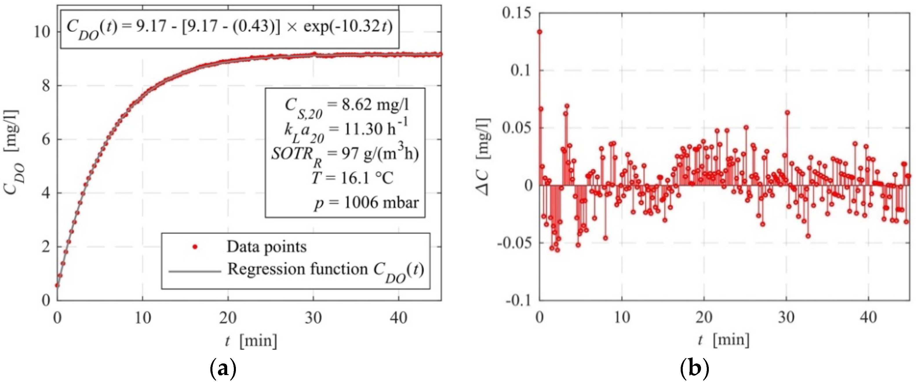
respectively. In Equation (10), CS,St,T refers to the standardized saturation concentration for p = 1013 hPa and temperature T, while CS,St,20 = 9.09 mg/L for full standard conditions. An exemplary result from a single oxygenation test is shown in Figure 3a. Figure 3b shows the residuals between the fitting and the laboratory data, proving a good fitting.
4. Results
4.1. Specific Air-Water Interface
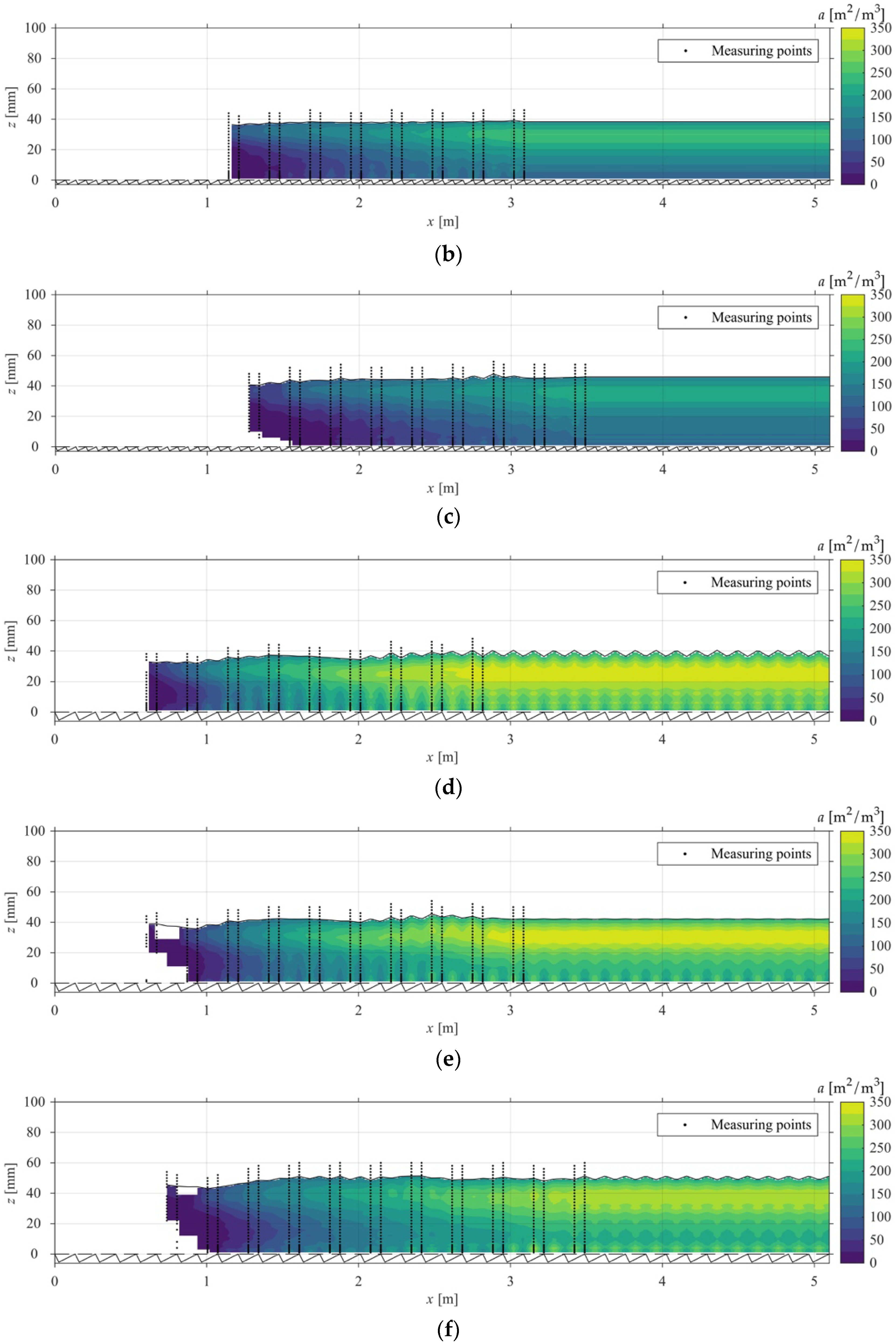
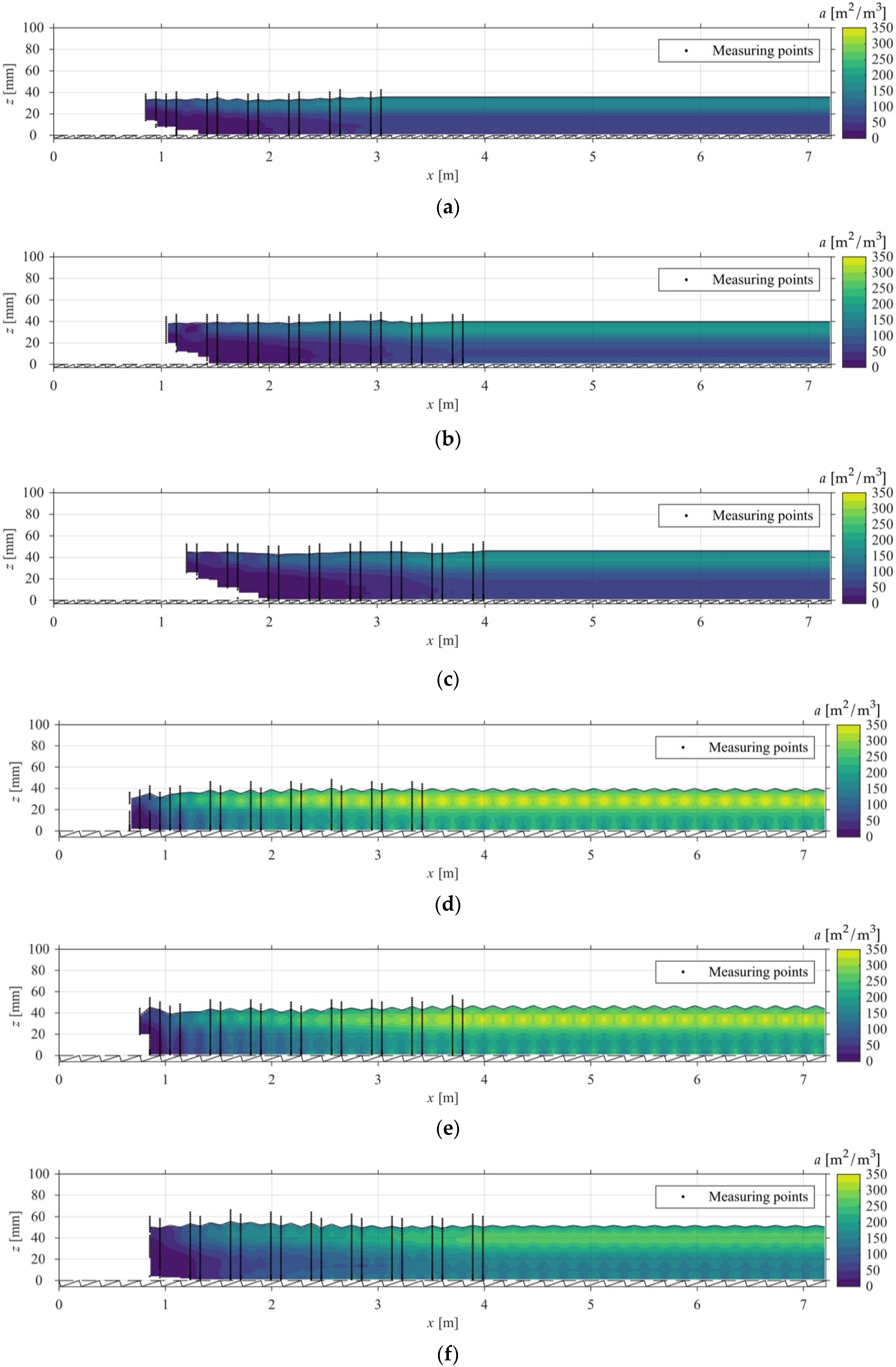
The specific air-water interface according to Equation (7) has been determined between the inception point of self-aeration and the quasi-uniform flow region for 0 ≤ z ≤ h75 in all configurations. The results in dimensional numbers are illustrated in Figure 4 for 1:2 slope and Figure 5 for 1:3 slope. It can be observed that the total amount strongly depends on the flow regime. While for smaller step heights and larger discharges a more stable skimming flow regime is found, a more tumbling flow is found for larger step heights and lower discharges. This leads to a more chaotic flow regime and stronger aeration. For all configurations, the specific air-water interface follows a distribution as shown in Figure 1b with a maximum slightly below h75. The highest air-water interfaces being observed in the current tests are in the order of 350 m2/m3.
In order to determine the gas transfer velocity from the aeration efficiencies (shown subsequently), the total air-water interface from entrained air bubbles is required and can be calculated by
where Li is the distance from the spillway crest to the inception point of self-aeration, Ltot is the total length of the spillway and b is the width of the flume. The resulting surface area of the supposed sinusoidal air-water mixture surface according to Equation (A7) is added to Aent from Equation (11) to determine the total available air-water Atot interface. Description of the assumed surface wave geometry and derivation of relevant functions is given in the Appendix A. Results for both interfaces Aent and , as well as the total air-water interface Atot from all the tested configurations, are listed in Table 2.
It is interesting to note that for less stable skimming flow regimes (i.e., for larger steps and lower discharges), the total air-water interface increases significantly with a relevant contribution of the surface waves. With consideration of this total surface Atot in Table 2 and the total water volume, consisting of the air-water mixture volume
plus the fluid volume beneath the surface waves for z > h75 according to Equation (A8) (tot = mix + ), the total specific air-water interface atot is found as follows in Table 3:
4.2. Re-Aeration Perfomance
Relevant re-aeration performance parameters are obtained by nonlinear regression of the oxygenation data, as shown in Figure 3. As the experiments have been conducted on different days with different local conditions, the standardized re-aeration parameters are always presented in the following. For each configuration, four independent model runs were performed and the averaged results for kLa20 and CS,20 are listed in Table 4.
4.3. Mass Transfer Velocity
The mass transfer coefficient can be directly deduced from Table 3 and Table 4. The results are shown in Table 5.
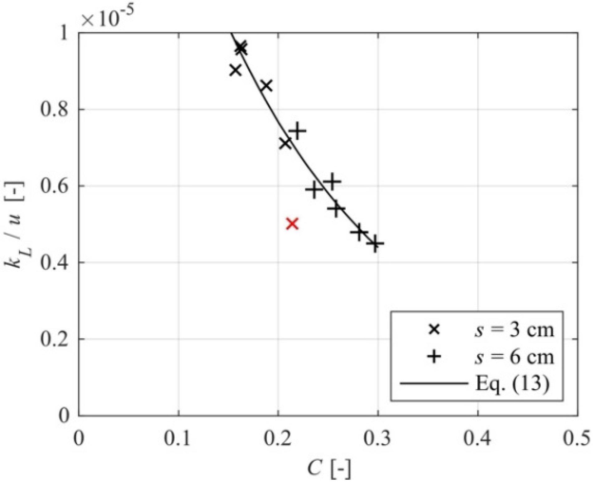
Obviously, kL increases for higher discharges and is thus a function of the Reynolds number. The flow regime (i.e., the stability of the skimming flow), which was affecting the specific air-water interface, is found to have no significant influence on kL. In addition, it is noticed that the air concentration strongly affects the mass transfer as well (as it was also described in [38] under consideration of an air-water mixture up to h90). With the average flow velocity u being found in the aerated flow region and the average air concentration on the structure (up to h75), the following relationship is found:
The curve fitting reaches R2 = 0.96 when neglecting a single obvious outlier, as indicated in Figure 6.
5. Discussion and Conclusions
The results underline that re-aeration on stepped spillways depends on the spillway geometry and discharge. While the amount of entrained air or specific air-water interface becomes higher for less stable skimming flow regimes, where the flow structure is more chaotic, the mass transfer is mainly a function of the mean flow velocity (being a measure of the Reynolds number and thus, the turbulence) and the mean air concentration. This result is supported by a similar finding published in [25]. Application of any mass transfer model with constant kL seems to be inaccurate for highly-aerated flows at hydraulic structures. It is shown that a proper consideration of the waved surface is essential, particularly for lower discharges. While the difference of specific air-water interface Aent between the present concept (mixture up to h75) and the concept applied in [38] (mixture up to h90 and neglecting of surface waves) was only in the order of 5%, the increase of Aent is found to be up to 65% when considering surface waves. The assumption of a sinusoidal, symmetrical wave field needs to be further investigated and improved in future by considering a wide spectrum of wavelengths and refined geometries.
All tests were conducted on a large scale model meeting the scale recommendations given in different studies (e.g., [48]) with a minimum Reynolds number of approximately 105 and a minimum Weber number of approximately 100. However, bubble sizes must be considered to be strongly affected by scale effects [49]. Thus, the presented results on air water interface due to entrained air bubbles cannot be directly transferred to different scales. Scale effects in regard to surface waves have not been investigated yet and require further attention. It is not clear if the mass transfer equation presented, that is, Equation (13), is affected by scale effects as well. The flow velocity and air concentration, which were found to be related to mass transfer, may be considered to be unaffected by scale effects due the large model scale. Distinguishing between bubbles and waves may help in understanding proper scaling of the flow structure and more accurate extrapolations to prototype scale.
Author Contributions
Conceptualization, D.B.B.; Formal analysis, D.B.B. and D.V.; Investigation, D.B.B.; Methodology, D.B.B.; Visualization, D.B.B. and D.V.; Writing—original draft, D.B.B.; Writing—review & editing, D.V.
Funding
This research received no external funding.
Acknowledgments
The first author acknowledges the support by Andreas Schlenkhoff, University of Wuppertal, Germany. All experimental data have been gathered in his laboratory during the Ph.D. thesis of the first author.
Conflicts of Interest
The authors declare no conflict of interest.
Appendix A. Assumption of a Three-Dimensional, Sinusoidal Surface Wave Field
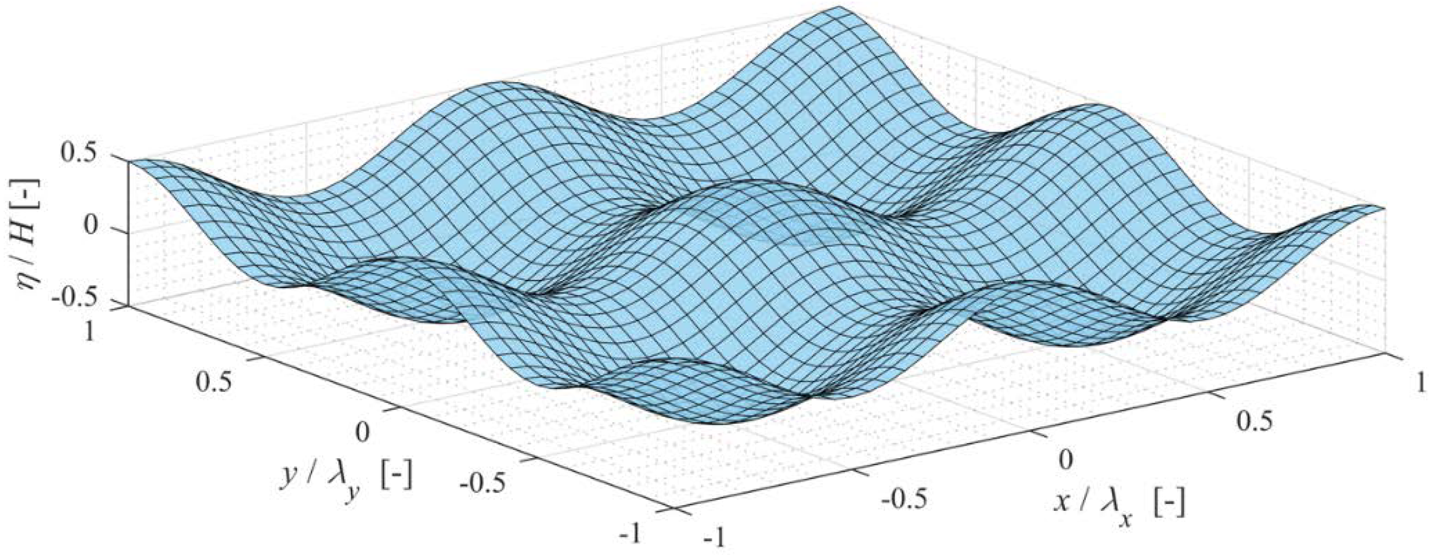
In this study, a three-dimensional sinusoidal wave field is assumed with a geometry given by
being the waveheight. is periodic in and (see Figure A1). For simplicity, is assumed to be homogeneous in both coordinates, thus leading to .
Figure A1.
Free surface waved profile simplification.

Applying simple trigonometric considerations, the arc length in the plane - is given by:
Likewise, for the - plane:
Altogether, the surface area will be given by:
With the last term (cross product of the differences) being of higher order (herein neglected) and :
The integral providing the surface area (Equation (A4)) has no closed form, but it can be approximated as a sum of finite differences ():
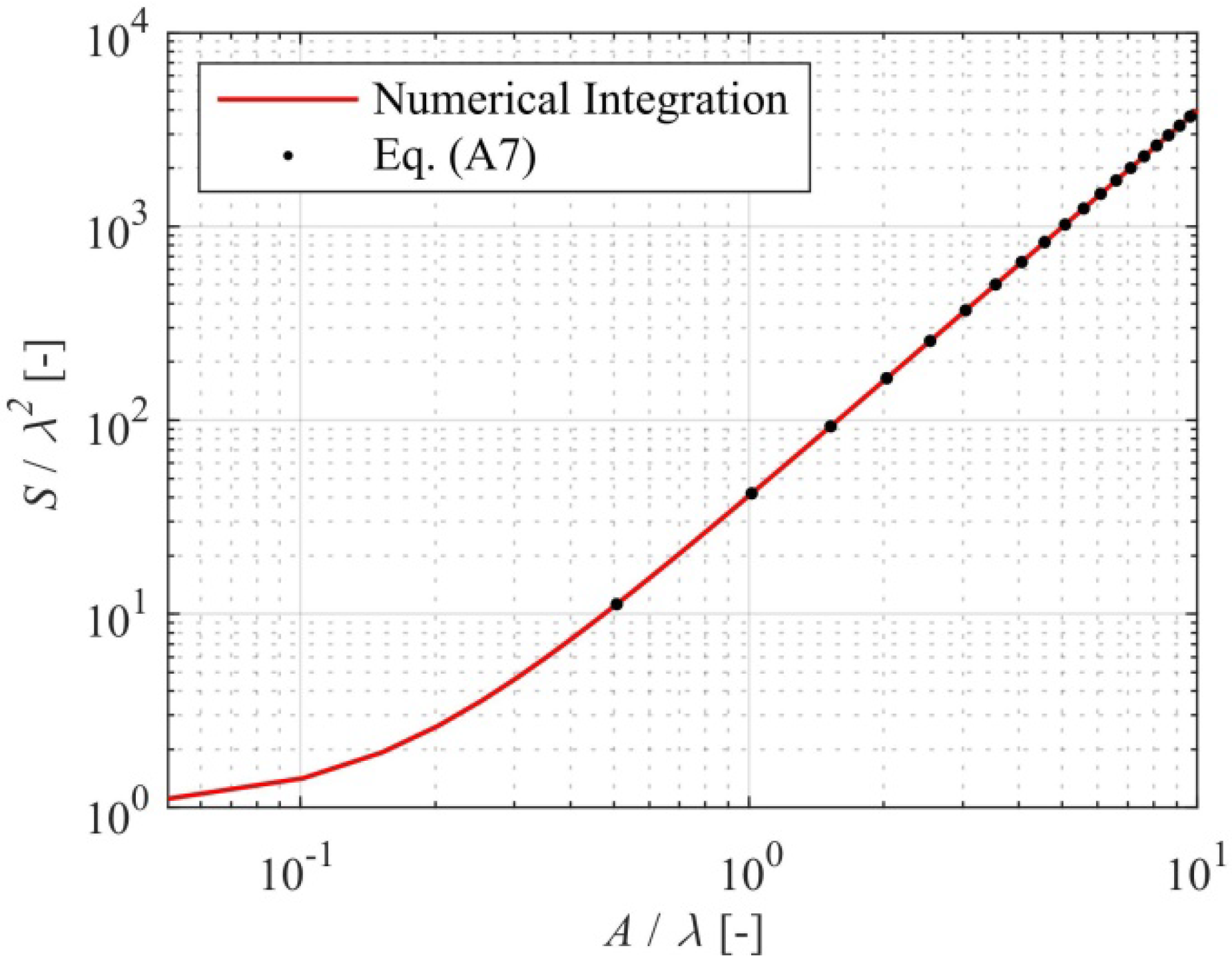
It is noteworthy that wave surface derivatives are exact (Equation (A3)) and only finite differences are used for and . Integrating over a periodic length-scale in both directions ( and ); result of Figure A2 can be obtained.
Figure A2.
Numerical integration of the waved interfacial surface for a squared region.

Being the approximation:
Note that = 0 yields = . Due to the symmetry in the vertical direction, the fluid volume beneath this surface wave field is given by Equation (2)
References
- Chanson, H.; Bung, D.B.; Matos, J. Stepped spillways and cascades. In Energy Dissipation in Hydraulic Structures; Chanson, H., Ed.; CRC Press: Leiden, The Netherlands, 2015; pp. 45–64. ISBN 978-1-138-02755-8. [Google Scholar] [Green Version]
- Valero, D.; Bung, D.B. Development of the interfacial air layer in the non-aerated region of high-velocity spillway flows. Instabilities growth, entrapped air and influence on the self-aeration onset. Int. J. Multiph. Flow 2016, 100, 66–74. [Google Scholar] [CrossRef]
- Valero, D.; Bung, D.B. Reformulating self-aeration in hydraulic structures: Turbulent growth of free surface perturbations leading to air entrainment. Int. J. Multiph. Flow 2018, 100, 127–142. [Google Scholar] [CrossRef]
- Chanson, H. The Hydraulics of Stepped Chutes and Spillways; A. A. Balkema: Lisse, The Nethererlands, 2002; ISBN 9058093522. [Google Scholar]
- Gameson, A.L.H. Weirs and Aeration of Rivers. J. Inst. Water Eng. 1957, 11, 477–490. [Google Scholar]
- Tebbutt, T.H.Y. Some studies on reaeration in cascades. Water Res. 1972, 6, 297–304. [Google Scholar] [CrossRef]
- Tebbutt, T.H.Y.; Essery, L.T.S.; Rasaratnam, S.K. Reaeration performance of stepped cascades. J. Inst. Water Eng. 1977, 31, 285–297. [Google Scholar]
- Avery, S.T.; Novak, P. Oxygen transfer at hydraulic structures. J. Hydraulics Div. 1978, 104, 1521–1540. [Google Scholar]
- Essery, I.T.S.; Tebutt, T.H.Y.; Rasaratnam, S.K. Design of Spillways for Re-Aeration of Polluted Waters; Construction Industry Research and Information Association (CIRIA): Birmingham, UK, 1978; ISBN 978-0860171102. [Google Scholar]
- Toombes, L.; Chanson, H. Air–water mass transfer on a stepped waterway. J. Environ. Eng. 2005, 131, 1377–1386. [Google Scholar] [CrossRef]
- Baylar, A.; Emiroglu, M.E.; Bagatur, T. An experimental investigation of aeration performance in stepped spillways. Water Environ. J. 2006, 20, 35–42. [Google Scholar] [CrossRef]
- Erpicum, S.; Lodomez, M.; Savatier, J.; Archambeau, P.; Dewals, B.; Pirotton, M. Physical modeling of an aerating stepped spillway. In Hydraulic Structures and Water System Management, Proceedings of the 6th IAHR International Symposium on Hydraulic Structures, Portland, OR, USA, 27–30 June 2016; Crookston, B., Tullis, B.P., Eds.; Utah State University: Logan, UT, USA, 2016; pp. 608–617. ISBN 978-1-884575-75-4. [Google Scholar] [CrossRef]
- Bung, D.B. Non-intrusive detection of air–water surface roughness in self-aerated chute flows. J. Hydraulic Res. 2013, 51, 322–329. [Google Scholar] [CrossRef]
- Killen, J.M. The Surface Characteristics of Self-Aerated Flow in Steep Channels. Ph.D. Thesis, University of Minnesota, Minneapolis, MN, USA, 1968. [Google Scholar]
- Wilhelms, S.C.; Gulliver, J.S. Bubbles and waves description of self-aerated spillway flow. J. Hydraulic Res. 2005, 43, 522–531. [Google Scholar] [CrossRef]
- Cussler, E.L. Diffusion: Mass Transfer in Fluid Systems; Cambridge University Press: Cambridge, UK, 1997; ISBN 0 521 29846 0. [Google Scholar]
- Lewis, W.K.; Whitman, W.G. Principles of Gas Absorption. J. Ind. Eng. Chem. 1924, 16, 1215–1220. [Google Scholar] [CrossRef]
- Westrich, B.; Haag, I. Modellgestützte Optimierung des Einsatzes Finanzieller Mittel Zur Verbesserung des Sauerstoffhaushalts Im Neckar; Technical Report; University of Stuttgart: Stuttgart, Germany, 2002. [Google Scholar]
- Higbie, R. The rate of absorption of a pure gas into a still liquid during a short time exposure. Trans. Am. Inst. Chem. Eng. 1935, 31, 365–389. [Google Scholar]
- Danckwerts, P.V. Significance of liquid-film coefficients in gas absorption. J. Ind. Eng. Chem. 1951, 43, 1460–1467. [Google Scholar] [CrossRef]
- Fortescue, G.E.; Pearson, J.R.A. On Gas Absorption into a Turbulent Liquid. Chem. Eng. Sci. 1967, 22, 1163–1176. [Google Scholar] [CrossRef]
- Lamont, J.C.; Scott, D.S. An eddy cell model of mass transfer into the surface of a turbulent liquid. AIChE 1970, 16, 513–519. [Google Scholar] [CrossRef]
- Moog, D.B.; Jirka, G.H. Macro-roughness effects on stream reaeration. In Hydraulic Engineering ’94, Proceedings of the 1994 ASCE Conference, Buffalo, NY, USA, 1–5 August 1994; Cotroneo, G.V., Rumer, R.R., Eds.; American Society of Civil Engineers: Reston, VA, USA, 1994; pp. 994–998. [Google Scholar]
- Gualtieri, C.; Gualtieri, P. Turbulence-based models for gas transfer analysis with channel shape factor influence. Environ. Fluid Mech. 2004, 4, 249–271. [Google Scholar] [CrossRef]
- Jun, K.S.; Jain, S.C. Oxygen transfer in bubbly turbulent shear flow. J. Hydraulic Eng. 1993, 119, 21–36. [Google Scholar] [CrossRef]
- Kawase, Y.; Moo-Young, M. Correlations for liquid-phase mass transfer coefficients in bubble column reactors with newtonian and non-newtonian fluids. Can. J. Chem. Eng. 1992, 70, 48–54. [Google Scholar] [CrossRef]
- Demars, B.O.L.; Manson, R.J. Temperature dependence of stream aeration coefficients and the effect of water turbulence: A critical review. Water Res. 2013, 47, 1–15. [Google Scholar] [CrossRef] [PubMed]
- Chanson, H. Measuring air-water interface area in supercritical open channel flows. Water Res. 1997, 31, 1414–1420. [Google Scholar] [CrossRef] [Green Version]
- Toombes, L. Experimental Study of Air-Water Flow Properties on Low-Gradient Stepped Cascades. Ph.D. Thesis, The University of Queensland, Brisbane, Australia, 2002. [Google Scholar]
- Toombes, L.; Chanson, H. Air-Water Flow and Gas Transfer at Aeration Cascades: A Comparative Study of Smooth and Stepped Chutes. In International Workshop on Hydraulics of Stepped Spillways (IAHR); Minor, H.-E., Hager, W.H., Eds.; A.A. Balkema: Zurich, Switzerland, 2000; pp. S77–S84. [Google Scholar]
- Cain, P. Measurements within Self-Aerated Flow on a Large Spillway. Ph.D. Thesis, University of Canterbury, Christchurch, New Zealand, 1978. [Google Scholar]
- Chanson, H. Study of Air Entrainment and Aeration Devices on Spillway Model. Ph.D. Thesis, University of Canterbury, Christchurch, New Zealand, 1988. [Google Scholar]
- Pegram, G.G.S.; Officer, A.K.; Mottram, S.R. Hydraulics of skimming flow on modeled stepped spillways. J. Hydraulic Eng. 1999, 125, 500–510. [Google Scholar] [CrossRef]
- André, S. High Velocity Aerated Flows on Stepped Chutes with Macro-Roughness Elements. Ph.D. Thesis, École Polytechnique Fédérale de Lausanne, Lausanne, Switzerland, 2004. [Google Scholar]
- Pfister, M.; Hager, W.H. Self-entrainment of air in stepped spillways. Int. J. Multiph. Flow 2011, 37, 99–107. [Google Scholar] [CrossRef]
- Bung, D.B.; Valero, D. Optical flow estimation in aerated flows. J. Hydraulic Res. 2016, 575–580. [Google Scholar] [CrossRef]
- Bung, D.B. Zur Selbstbelüfteten Gerinneströmung Auf Kaskaden Mit Gemässigter Neigung; Shaker: Aachen, Germany, 2009; ISBN 978-3-8322-8382-7. [Google Scholar]
- Schlenkhoff, A.; Bung, D.B. Prediction of the oxygen transfer in self-aerated skimming flow on embankment stepped spillways. In Proceedings of the 33rd IAHR World Congress “Water Engineering for a Sustainable Environment”, Vancouver, BC, Canada, 9–14 August 2009. [Google Scholar]
- Bung, D.B. Fließcharakteristik und Sauerstoffeintrag bei selbstbelüfteten Gerinneströmungen auf Kaskaden mit gemäßigter Neigung. Österreichische Wasser- und Abfallwirtschaft 2011, 63, 76–81. [Google Scholar] [CrossRef]
- Bung, D.B. Developing flow in skimming flow regime on embankment stepped spillways. J. Hydraulic Res. 2011, 49, 639–648. [Google Scholar] [CrossRef]
- Boes, R.M.; Hager, W.H. Hydraulic design of stepped spillways. J. Hydraulic Eng. 2003, 129, 671–679. [Google Scholar] [CrossRef]
- Chanson, H.; Toombes, L. Hydraulics of stepped chutes: The transition flow. J. Hydraulic Res. 2004 42, 43–54. [CrossRef] [Green Version]
- Yasuda, Y.; Ohtsu, I. Flow Resistance of Skimming Flows in Stepped Channels. In Hydraulic Engineering for Sustainable Water Resources Management at the Turn of the Millenium, Proceedings of the 28th IAHR World Congress, Graz, Austria, 22–27 August 1999; Technical University Graz: Graz, Austria, 1999. [Google Scholar]
- Bung, D.B. Sensitivity of phase detection techniques in aerated chute flows to hydraulic design parameters. In Proceedings of the 2nd IAHR Europe Congress, Munich, Germany, 27–29 June 2012. [Google Scholar]
- Chanson, H. Air-water flow measurements with intrusive, phase-detection probes: Can we improve their interpretation? J. Hydraulic Eng. 2002, 128, 252–255. [Google Scholar] [CrossRef]
- Bung, D.B. Air-water surface roughness in self-aerated stepped spillway flows. In Proceedings of the 35th IAHR World Congress, Chengdu, China, 8–13 September 2013. [Google Scholar]
- American Society of Civil Engineers. Measurement of Oxygen Transfer in Clean Water; American Society of Civil Engineers: Reston, VA, USA, 2007. [Google Scholar]
- Boes, R.M.; Hager, W.H. Two-phase flow characteristics of stepped spillways. J. Hydraulic Eng. 2003, 129, 661–670. [Google Scholar] [CrossRef]
- Felder, S.; Chanson, H. Scale effects in microscopic air-water flow properties in high-velocity free-surface flows. Exp. Therm. Fluid Sci. 2017 83, 19–36. [CrossRef]
Figure 1.
Flow structure in stepped spillway flows: (a) High-speed video frame taken for slope 1:2, s = 6 cm, q = 0.07 m2/s, and h75 determined with the conductivity probe; (b) distribution of the dimensionless air-water interface a/max(a) according to Equation (7). Shading of the markers from black (at the inception point of self-aeration) to white (at the onset of quasi-uniform flow).

Figure 2.
Schematic illustration of the considered flow structure over the step cavities consisting of a continuous air-water mixture up to h75 and non-aerated, sinusoidal surface waves over h75.
Figure 2.
Schematic illustration of the considered flow structure over the step cavities consisting of a continuous air-water mixture up to h75 and non-aerated, sinusoidal surface waves over h75.

Figure 3.
Exponential regression of oxygenation curves for one exemplary model run with 1:2 slope, s = 6 cm and q = 0.11 m2/s: (a) Fitting to the experimental data for local conditions and resulting standardized oxygen transfer parameters (note: only every 2nd data point is shown for better legibility); (b) Residuals resulting from the curve fitting.

Figure 4.
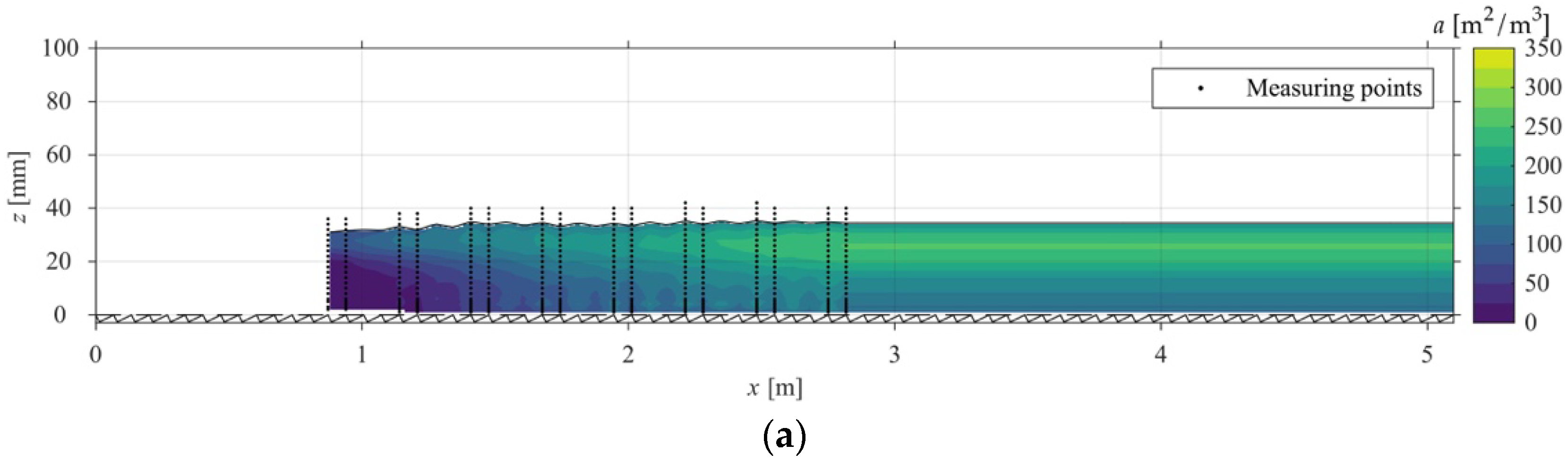
Specific air-water interface a (in m2/m3) for all configurations with slope 1:2; downstream of the inception point of self-aeration and from z = 0 (pseudo-bottom) to h75; data in quasi-uniform flow region assumed similar to the last two profiles: (a) s = 3 cm, q = 0.07 m2/s; (b) s = 3 cm, q = 0.09 m2/s; (c) s = 3 cm, q = 0.11 m2/s; (d) s = 6 cm, q = 0.07 m2/s; (e) s = 6 cm, q = 0.09 m2/s; (f) s = 6 cm, q = 0.11 m2/s.
Figure 4.
Specific air-water interface a (in m2/m3) for all configurations with slope 1:2; downstream of the inception point of self-aeration and from z = 0 (pseudo-bottom) to h75; data in quasi-uniform flow region assumed similar to the last two profiles: (a) s = 3 cm, q = 0.07 m2/s; (b) s = 3 cm, q = 0.09 m2/s; (c) s = 3 cm, q = 0.11 m2/s; (d) s = 6 cm, q = 0.07 m2/s; (e) s = 6 cm, q = 0.09 m2/s; (f) s = 6 cm, q = 0.11 m2/s.


Figure 5.
Specific air-water interface a (in m2/m3) for all configurations with slope 1:3; downstream of the inception point of self-aeration and from z = 0 (pseudo-bottom) to h75; data in quasi-uniform flow region assumed similar to the last two profiles: (a) s = 3 cm, q = 0.07 m2/s; (b) s = 3 cm, q = 0.09 m2/s; (c) s = 3 cm, q = 0.11 m2/s; (d) s = 6 cm, q = 0.07 m2/s; (e) s = 6 cm, q = 0.09 m2/s; (f) s = 6 cm, q = 0.11 m2/s.

Figure 6.
Relative mass transfer velocity kL/u as a function of the mean air concentration (the red marker results from the configuration with 1:2 slope, s = 3 cm step height and q = 0.07 m2/s discharge and has been neglected for the curve fitting).
Figure 6.
Relative mass transfer velocity kL/u as a function of the mean air concentration (the red marker results from the configuration with 1:2 slope, s = 3 cm step height and q = 0.07 m2/s discharge and has been neglected for the curve fitting).


Table 1.
Median wavelengths and waveheights extracted from high-speed videos with use of an image processing technique; corresponding median absolute deviations (MAD) given in brackets.
Table 1.
Median wavelengths and waveheights extracted from high-speed videos with use of an image processing technique; corresponding median absolute deviations (MAD) given in brackets.
| Slope 1:2 | Slope 1:3 | |||||||||||
|---|---|---|---|---|---|---|---|---|---|---|---|---|
| Step Height [cm] | 3 | 6 | 3 | 6 | ||||||||
| Discharge [m2/s] | 0.07 | 0.09 | 0.11 | 0.07 | 0.09 | 0.11 | 0.07 | 0.09 | 0.11 | 0.07 | 0.09 | 0.11 |
| λ [cm] | 6.1 (1.6) | 7.5 (1.4) | 8.9 (2.3) | 7.1 (1.7) | 7.3 (1.4) | 6.6 (1.8) | 6.7 (1.3) | 5.9 (1.2) | 7.1 (1.9) | 5.9 (1.3) | 5.7 (1.1) | 6.6 (1.6) |
| H [cm] | 1.4 (0.6) | 1.3 (0.8) | 1.3 (0.6) | 2.6 (1.0) | 2.0 (1.3) | 2.1 (1.1) | 1.3 (0.8) | 1.3 (0.5) | 1.2 (0.7) | 3.9 (1.4) | 3.1 (1.2) | 2.9 (1.2) |
Table 2.
Total air-water interface for all configurations.
| Slope 1:2 | Slope 1:3 | |||||||||||
|---|---|---|---|---|---|---|---|---|---|---|---|---|
| Step Height [cm] | 3 | 6 | 3 | 6 | ||||||||
| Discharge [m2/s] | 0.07 | 0.09 | 0.11 | 0.07 | 0.09 | 0.11 | 0.07 | 0.09 | 0.11 | 0.07 | 0.09 | 0.11 |
| Entrained air bubbles Aent [m2] (Equation (11)) | 7.37 | 7.31 | 6.93 | 12.67 | 12.60 | 13.21 | 5.65 | 7.05 | 6.89 | 17.58 | 18.32 | 16.06 |
| Air-water mixture surface [m2] (Equation (A7)) | 1.95 | 1.58 | 1.34 | 3.24 | 2.29 | 2.58 | 2.55 | 2.62 | 2.06 | 10.67 | 7.88 | 5.71 |
| Atot [m2] | 9.32 | 8.89 | 8.27 | 15.91 | 14.89 | 15.79 | 8.20 | 9.67 | 8.95 | 28.25 | 26.20 | 21.77 |
Table 3.
Total specific air-water interface for all configurations.
| Slope 1:2 | Slope 1:3 | |||||||||||
|---|---|---|---|---|---|---|---|---|---|---|---|---|
| Step Height [cm] | 3 | 6 | 3 | 6 | ||||||||
| Discharge [m2/s] | 0.07 | 0.09 | 0.11 | 0.07 | 0.09 | 0.11 | 0.07 | 0.09 | 0.11 | 0.07 | 0.09 | 0.11 |
| atot [m2/m3] | 150 | 132 | 106 | 197 | 190 | 177 | 91 | 98 | 81 | 223 | 196 | 153 |
Table 4.
Standardized re-aeration performance parameters for all configurations (each averaged from four independent model runs, corresponding minimum and maximum values given in brackets).
Table 4.
Standardized re-aeration performance parameters for all configurations (each averaged from four independent model runs, corresponding minimum and maximum values given in brackets).
| Slope 1:2 | Slope 1:3 | |||||||||||
|---|---|---|---|---|---|---|---|---|---|---|---|---|
| Step Height [cm] | 3 | 6 | 3 | 6 | ||||||||
| Discharge [m2/s] | 0.07 | 0.09 | 0.11 | 0.07 | 0.09 | 0.11 | 0.07 | 0.09 | 0.11 | 0.07 | 0.09 | 0.11 |
| kLa20 [1/h] | (6.71) 6.85 (7.04) | (9.27) 9.32 (9.41) | (9.39) 9.76 (10.13) | (8.51) 8.73 (8.87) | (11.61) 11.68 (11.81) | (10.53) 11.11 (11.49) | (6.56) 7.54 (11.33) | (8.14) 8.87 (11.33) | (9.74) 10.17 (11.33) | (7.74) 8.60 (11.33) | (9.40) 10.08 (11.33) | (10.92) 11.47 (11.89) |
| CS,20 [mg/L] | (8.44) 8.61 (8.77) | (8.57) 8.68 (8.78) | (8.60) 8.70 (8.70) | (8.46) 8.63 (8.80) | (8.54) 8.67 (8.79) | (8.61) 8.75 (8.95) | (8.29) 8.43 (8.61) | (8.39) 8.48 (8.61) | (8.41) 8.48 (8.61) | (8.26) 8.42 (8.61) | (8.31) 8.43 (8.61) | (8.34) 8.53 (8.86) |
Table 5.
Deduced mass transfer velocities for all configurations.
| Slope 1:2 | Slope 1:3 | |||||||||||
|---|---|---|---|---|---|---|---|---|---|---|---|---|
| Step Height [cm] | 3 | 6 | 3 | 6 | ||||||||
| Discharge [m2/s] | 0.07 | 0.09 | 0.11 | 0.07 | 0.09 | 0.11 | 0.07 | 0.09 | 0.11 | 0.07 | 0.09 | 0.11 |
| kL [cm/h] | 4.6 | 7.1 | 9.2 | 4.4 | 6.1 | 6.3 | 8.3 | 9.1 | 12.6 | 3.9 | 5.1 | 7.5 |
© 2018 by the authors. Licensee MDPI, Basel, Switzerland. This article is an open access article distributed under the terms and conditions of the Creative Commons Attribution (CC BY) license (http://creativecommons.org/licenses/by/4.0/).
Share and Cite
MDPI and ACS Style
Bung, D.B.; Valero, D. Re-Aeration on Stepped Spillways with Special Consideration of Entrained and Entrapped Air. Geosciences 2018, 8, 333. https://doi.org/10.3390/geosciences8090333
AMA Style
Bung DB, Valero D. Re-Aeration on Stepped Spillways with Special Consideration of Entrained and Entrapped Air. Geosciences. 2018; 8(9):333. https://doi.org/10.3390/geosciences8090333
Chicago/Turabian StyleBung, Daniel B., and Daniel Valero. 2018. "Re-Aeration on Stepped Spillways with Special Consideration of Entrained and Entrapped Air" Geosciences 8, no. 9: 333. https://doi.org/10.3390/geosciences8090333
Note that from the first issue of 2016, this journal uses article numbers instead of page numbers. See further details here.