Numerical Modeling of Flow Patterns Applied to Analysis of Susceptibility to Movements of the Ground

Abstract

Mass movements in deformed areas of natural relief deformed by seismotectonic factors are one of the most destructive and recurrent natural hazards in the Republic of Ecuador, especially during intense rain periods, the El Niño phenomenon, or due to earthquakes such as the one that occurred on 16 April 2016 in the Ecuadorian coastline. This study proposes the application of Hydrological Model D8 and its derived morphometric parameters like slope, orientation of the slope, and curvatures, extracted from the high spatial resolution Digital Elevation Model (DEM), implemented in programs such as Rockworks 7 (gridzo), SURFER (downwards slope), ArcView (flowacc), and SAGA (curvatures) to obtain runoff flow, structural geological lineaments, and superficial deformations of the topographic relief that are the origin of erosion, superficial landslides, lateral propagation, of the rock–soil complex, mass flows, and deep gravitational deformations. This methodology has been validated in three locations with intense deformations: two in Ecuador and one in Spain. The DEM were obtained from the Ecuadorian Spatial Institute (ESI) (spatial resolution of 10 m), the Rural Technological Infrastructure and Information National System (SIGTIERRAS) (spatial resolution of 5 m), and the Council of Andalusia (spatial resolution of 5 m).

1. Introduction

Mass movements in Ecuador are one of the biggest threats that cause recurring disasters, especially during the periods of intense anomalous rains, the El Niño phenomenon, and earthquakes such as the one that occurred on April 16, 2016 in the Ecuadorian coastline.

In 2010, with the creation of the National Secretariat for Risk Management (SNGR), a standardized methodology was developed to elaborate mass movements’ susceptibility maps at a municipal level in the entire country using a 1:50,000 scale. This methodology was based on heuristic techniques, taking in consideration a number of variables based on the experience of researchers that have studied these types of risks over a period of several years, and their respective support documents, such as: Generation of Geoinformation for the Valoration of Territory at a National Level, component 3 Geopedology and Geological Risks project developed by the National Secretariat of Planification (SENPLADES); Initial Methodology for the elaboration of preliminary susceptibility maps to mass movements at a 1:50,000 scale, prepared by SNGR-SUN MONTAIN; and Mass Movements in the Andean Region: A Guide for Risk Evaluation, from the Multinational Andean Project (2000–2008).

This cartography identified susceptibility areas as intensity spots in a range going from absence of susceptibility to very high susceptibility and related these susceptible areas as regional geological structures; however, it wasn’t able to define structural lineaments, fractures, or topographic relief deformations that are the origin of mass movements and their different types. Based on the need to find these origins in better detail, the methodologic proposal was developed in relation to the outline of flow lines belonging to the superficial runoff of precipitation water as a mass pusher, structural geological lineaments, fractures, and deformations of the topographic relief from high mountainous areas, intermediate, and lower topographic areas. The numerical method applied is based on the theoretical principles of the D8 Hydrological Model, using Digital Elevation Models (DEM). The model was implemented in mathematical algorithms in programs such as Rockworks 7 (gridzo), SURFER (downward slope), ArcView (flowacc), and SAGA (curvatures).

One of the most important databases on which procedures to calculate hydrological parameters are based is the DEM. It is a data structure that represents the spatial distribution of a quantitative and continuous variable, the topography. DEMs are very efficient in extracting a big part of the necessary morphometric parameters to create a hydrological analysis in algorithms that several authors have developed to obtain the flow direction where each DEM cell is headed, calculate flow accumulation, draw flow lines or drainage networks, delimit the hydrography basin from the identification of an exit point, divide hydrographic basins in sub-basins, and calculate the morphometric properties of these hydrographic basins and drainage networks. Since 1994, most of studies focused on determining the flow paths of the superficial runoff of precipitation water and other mentioned products based on the D8 Model, but didn’t focus on the tracing lines of morphological fissures, nor structural geological lineaments and topographic deformation areas, despite models being integrated in slope stabilization computer programs with stabilization criteria such as SINMAP, ShalStab, and Tardem, among others.

The investigation of direction and flow-line tracing of the superficial runoff has its theoretical origins in various studies [1,2,3]. In this paper, the investigation about this topic started in 1996 and was based mainly on the investigation studies of several authors [2] about the application of digital-terrain models in natural sciences. Studies that served to understand the basic concepts of digital terrain models (DTM), emphasizing the definition, structure, and errors of the construction of the DEM, as well as its applications in the characterization of reliefs, preparation of topographic profiles, visualization and drainage of hydrographic basins, and elaborations of flow lines using the hydrological model D8 as a basic model.

The results of this investigation were presented in the First International Symposium of Mass Movements in Cuenca, Ecuador in 2001, at the conference ‘Flow paths as mass-movement generators: a vectorial focus‘[4]. Later, these results were presented at GeoSpatial World 2002 in Atlanta, Georgia, United States, in the conference ‘MGE as a support base for the construction of the morphologic breakage model^®’ in the geographic information systems (GIS) and environmental management chapter, summary 186 [5].

Since 2001, this model has been presented in several countries such as Chile [6], Cuba [7], and Spain [8]. This method has since been applied in Ecuador [9]. In later years, several researchers have completed and published a number of studies about this topic [10,11,12,13,14,15,16]. In the last decade, authors have investigated the analysis of structural lineaments based on stereoscopic interpretation with airborne radar images and satellites used in the oil industry, aquifers, and mineral-deposit exploration. An example is the focus of the Analysis of Guidelines for the Exploration of Groundwater in Nicaragua based on the analysis of crossed fractured networks using images from four satellite sensors (ASTER, Landsat-e ETM, QuickBird, RADARSAT-1) and 20 m spatial resolution DEM [17].

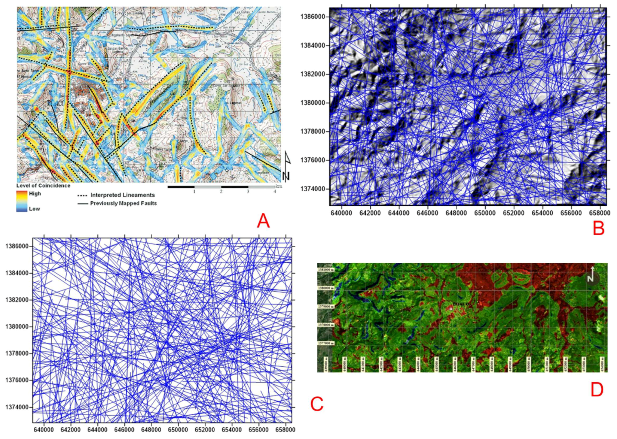
This analysis required a large amount of processing and interpretation time of the 12 images to draw the structural guidelines. Unlike the methodology that uses satellite images, the present methodology to extract guidelines or structural geological lineaments and relief deformations has quick processing time, high precision, and it uses free digital elevation models. In the following images, the structural guidelines are shown with the two methodologies applied to the same area (Nicaragua) with the same 20 m spatial resolution digital elevation model. In Figure 1A, the results of the coincidence between the guidelines obtained by remote sensing are shown. Figure 1B presents the structural guidelines obtained by the proposed method of this investigation. Figure 1C shows the coincidences and advantages of the proposed method; in addition to extracting structural guidelines and higher density fractures, relief deformations are also extracted by concentration of these lineaments, as can be evidenced in Figure 1D.

2. Materials and Methods

In order to extract the flow-path direction and its layout, structural geological guidelines, fractures, and superficial relief deformations, the theory of the basic Hydrological Model 8D was applied with high-resolution digital elevation models obtained from specialized institutions such as Telespazio (radar images), Cosmo SkyMed (10 m spatial resolution, Zone 1), Sigtierras (radar images, 3 m spatial resolution, Zone 2), and the Council of Andalusia (5 m spatial resolution, Zone 3). The used DEM were corrected before analysis. The used coordinate systems were UTM and WGS84-Zone 17S for the Ecuadorian studied areas, and UTM-Zone 30 and ETRS89 in Spain.

The used DEM were processed with public-use programs such as SAGA [18], ArcView [19] and commercial software like Rockworks 7 [20] and Surfer [21] to obtain the superficial water-runoff flow paths, structural geological lineaments, morphologic rupture lines, and deformations of the topographic relief. The realized fieldwork (300 control points) allowed us to verify the response of this methodology and collect data in susceptible sectors as well as types of associated mass movements. The operation of the basic Hydrological Model D8 and the determination of the direction and tracing of the surface runoff flows from precipitation are explained in the process diagram of Figure 2.

The first derived products of the application of the D8 Model in the DEM were the direction and tracing of the runoff flow paths from the rain surface, which are the base of the information needed to obtain the following products: structural geological lineaments, fractures, and surface relief deformations of erosive and seismotectonic origin.

The calculation of flow directions and line tracing represents that each cell of the digital elevation model is the starting point to find hydrological characteristics in the topographic relief. From the topographic surface, a raster was generated that showed the flow directions and the exit direction of each line of each cell is drawn. Each valid exit direction is related with each adjacent cell where the flow can travel. This approach is commonly known as the eight-way flow (D8) [1,2,3].

Flow direction is determined by the steepest-descent direction or the maximum fall from each cell, and it is calculated as follows (Equation (1)):

P = (Arctg(Z0 − Z1)/d)

(1)

where P: maximum fall, Z0−Z1: change of elevation value, and d: distance between each cell center. As distance is calculated between cell centers, if the cell size is 1, the distance between two orthogonal cells is 1 (creating an isosceles triangle). The distance between these two diagonal cells if √2 = 1.414. It may occur in this process that, when the maximum descent of various cells is the same, nearby sectors grow until the steepest descent and the flow direction of the cell are codified with the value that represents the mentioned direction. If all next elements are higher than the processing cell, it is considered a sink that fills with the lower value of the following elements and has a flow direction towards the mentioned cell. However, if a cell is next to the physical edge of the DEM or has at least a NoData cell as a neighbor, it doesn’t fill or doesn’t have value because the neighbor’s data are insufficient to be considered a true cell and a true flow and cell receptor. In order to be a receptor, the information around the cell has to be present to continue the process [22].

This procedure was applied to each cell of the DEM, Cn (I,j), with the exception of the borders and their 8 neighbors. Thus, water that enters a cell can exit through one of the 8 mentioned directions.

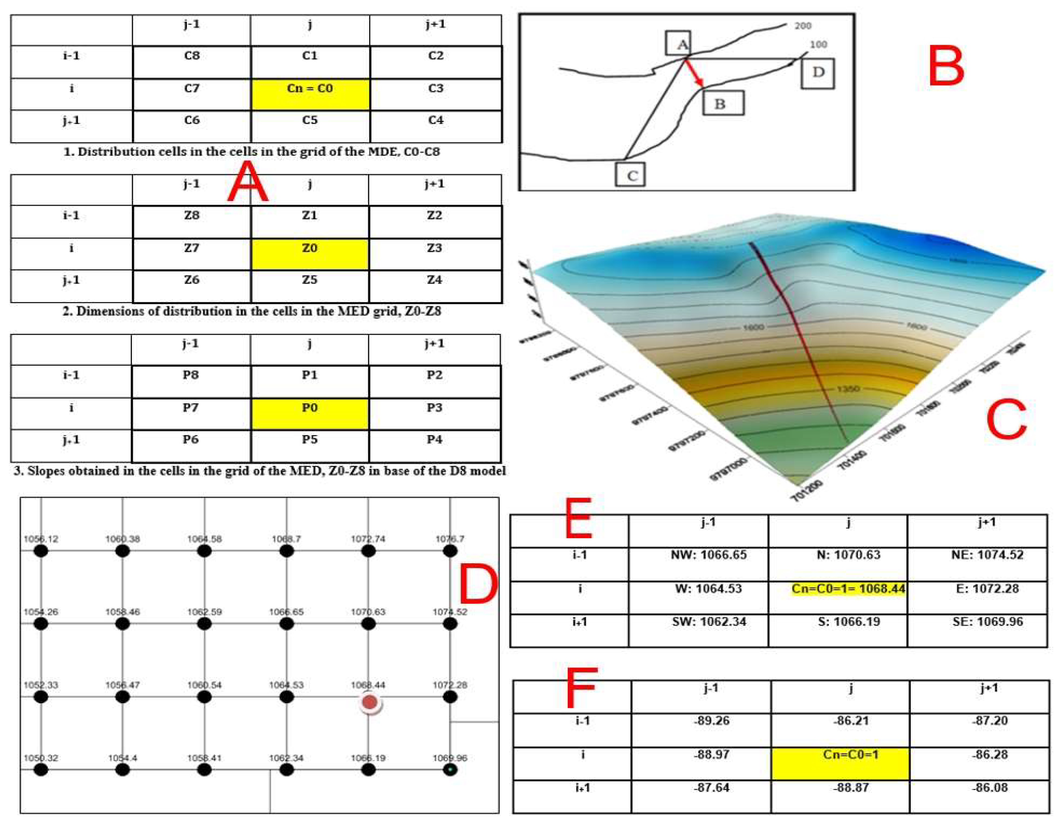
Workflow starts from a C0 cell (painted in yellow) with height starting point Z0. For each cell from C1 to C8 in a mesh, of designated heights by the DEM, slope P is calculated for each one of its neighbors to the north, northeast, east, southeast, south, southwest, west and northwest, as it is shown in Figure 3A. The objective of this process is to calculate the tangent of the angle formed by the horizontal with the line that joins the point under study with the neighbor that is the direction of the flow (Figure 3). The process is completed using Equation (2) (Figure 3B):

$$\begin{array}{c}\mathrm{P}1=\mathrm{Arctg}\left(\mathrm{Z}0-\mathrm{Z}1\right)/\surd 2\left(\mathrm{d}\right);\mathrm{P}2=\mathrm{Arctg}\left(\mathrm{Z}0-\mathrm{Z}2\right)/\surd 2\left(\mathrm{d}\right);\mathrm{P}3=\mathrm{Arctg}\left(\mathrm{ZO}-\mathrm{Z}3\right)/\surd 2\left(\mathrm{d}\right)\\ \mathrm{P}4=\mathrm{Arctg}\left(\mathrm{Z}0-\mathrm{Z}4\right)/\surd 2\left(\mathrm{d}\right);\mathrm{P}5=\mathrm{Arctg}\left(\mathrm{Z}0-\mathrm{Z}5\right)\surd 2\left(\mathrm{d}\right);\mathrm{P}6=\mathrm{Arctg}\left(\mathrm{Z}0-\mathrm{Z}6\right)/\surd 2\left(\mathrm{d}\right)\\ \mathrm{P}7=\mathrm{Arctg}\left(\mathrm{Z}0-\mathrm{Z}7\right)/\surd 2\left(\mathrm{d}\right);\mathrm{P}8=\mathrm{Arctg}\left(\mathrm{Z}0-\mathrm{Z}8\right)/\surd 2\left(\mathrm{d}\right)\end{array}$$

(2)

In Figure 3C, you can see how the maximum-slope line is drawn (maximum fall) inside the DEM. In a 10 m spatial resolution DEM, represented by the grid in Figure 3D, the lowest point is 750 masl. The construction of a morphologic flow and a rupture line from an initial C0 cell is carried out in 4 phases:

In Phase 1, the initial point of the line is established in a time t = 0, with the initial state C0 = 1, and assigned height by the DEM = 1068.44 m. Figure 3E,F shows the configuration of the data and their spatial position in the E, SE, NE, N, NW, W, or SW directions from the starting cell C0 (i,j).

In Phase 2, the slopes are calculated towards the 8 nearest neighbors, from the C0 cell towards the C1, C2, C3, C4, C5, C6, C7 and C8 cells, according to the local slope obtained from the slope map calculated with Equation (1), where d is the horizontal distance between the cells, which is 10 m in this study. This calculation was completed in the base of the previous equations. Orthogonal distance d from orthogonal cell centers is 1, and the distance between two diagonal cells is $\surd 2$ = 1.414 (Equation (3)):

$$\begin{array}{c}\mathrm{P}1=\mathrm{Atan}\left(\left(\mathrm{Abs}\left(-\mathrm{Z}0\right)-\mathrm{Abs}\left(\mathrm{Z}1\right)\right)/\left(\left(\surd 2\right)\mathrm{d}\right)\right)\to \mathrm{P}1=\mathrm{Atan}\left(\left(1068.44-1070.63\right)/\surd 2\times 10\right)=-86.21\\ \mathrm{P}2=\mathrm{Atan}\left(\left(\mathrm{Abs}\left(-\mathrm{Z}0\right)-\mathrm{Abs}\left(\mathrm{Z}2\right)\right)/\left(\left(\surd 2\right)\mathrm{d}\right)\right)\to \mathrm{P}2=\mathrm{Atan}(\left(1068.44-1074.52\right)/\surd 2\times 10=-87.20\\ \mathrm{P}3=\mathrm{Atan}\left(\left(\mathrm{Abs}\left(-\mathrm{Z}0\right)-\mathrm{Abs}\left(\mathrm{Z}3\right)\right)/\left(\left(\surd 2\right)\mathrm{d}\right)\right)\to \mathrm{P}3=\mathrm{Atan}(\left(1068.44-1072.28\right)/\surd 2\times 10=-89.28\\ \mathrm{P}4=\mathrm{Atan}\left(\left(\mathrm{Abs}\left(-\mathrm{Z}0\right)-\mathrm{Abs}\left(\mathrm{Z}4\right)\right)/\left(\left(\surd 2\right)\mathrm{d}\right)\right)\to \mathrm{P}4=\mathrm{Atan}(\left(1068.44-1069.96\right)/\surd 2\times 10=-89.08\\ \mathrm{P}5=\mathrm{Atan}\left(\left(\mathrm{Abs}\left(-\mathrm{Z}0\right)-\mathrm{Abs}\left(\mathrm{Z}5\right)\right)/\left(\left(\surd 2\right)\mathrm{d}\right)\right)\to \mathrm{P}5=\mathrm{Atan}(\left(1068.44-1066.19\right)/\surd 2\times 10=-88.87\\ \mathrm{P}6=\mathrm{Atan}\left(\left(\mathrm{Abs}\left(-\mathrm{Z}0\right)-\mathrm{Abs}\left(\mathrm{Z}6\right)\right)/\left(\left(\surd 2\right)\mathrm{d}\right)\right)\to \mathrm{P}6=\mathrm{Atan}(\left(1068.44-1062.34\right)/\surd 2\times 10=-87.64\\ \mathrm{P}7=\mathrm{Atan}\left(\left(\mathrm{Abs}\left(-\mathrm{Z}0\right)-\mathrm{Abs}\left(\mathrm{Z}7\right)\right)/\left(\left(\surd 2\right)\mathrm{d}\right)\right)\to \mathrm{P}7=\mathrm{Atan}(\left(1068.44-1064.53\right)/\surd 2\times 10=-88.97\\ \mathrm{P}8=\mathrm{Atan}\left(\left(\mathrm{Abs}\left(-\mathrm{Z}0\right)-\mathrm{Abs}\left(\mathrm{Z}8\right)\right)/\left(\left(\surd 2\right)\mathrm{d}\right)\right)\to \mathrm{P}8=\mathrm{Atan}(\left(1068.44-1066.65\right)/\surd 2\times 10=-89.26\end{array}$$

(3)

The spatial distribution of the slopes can be seen in Figure 3F.

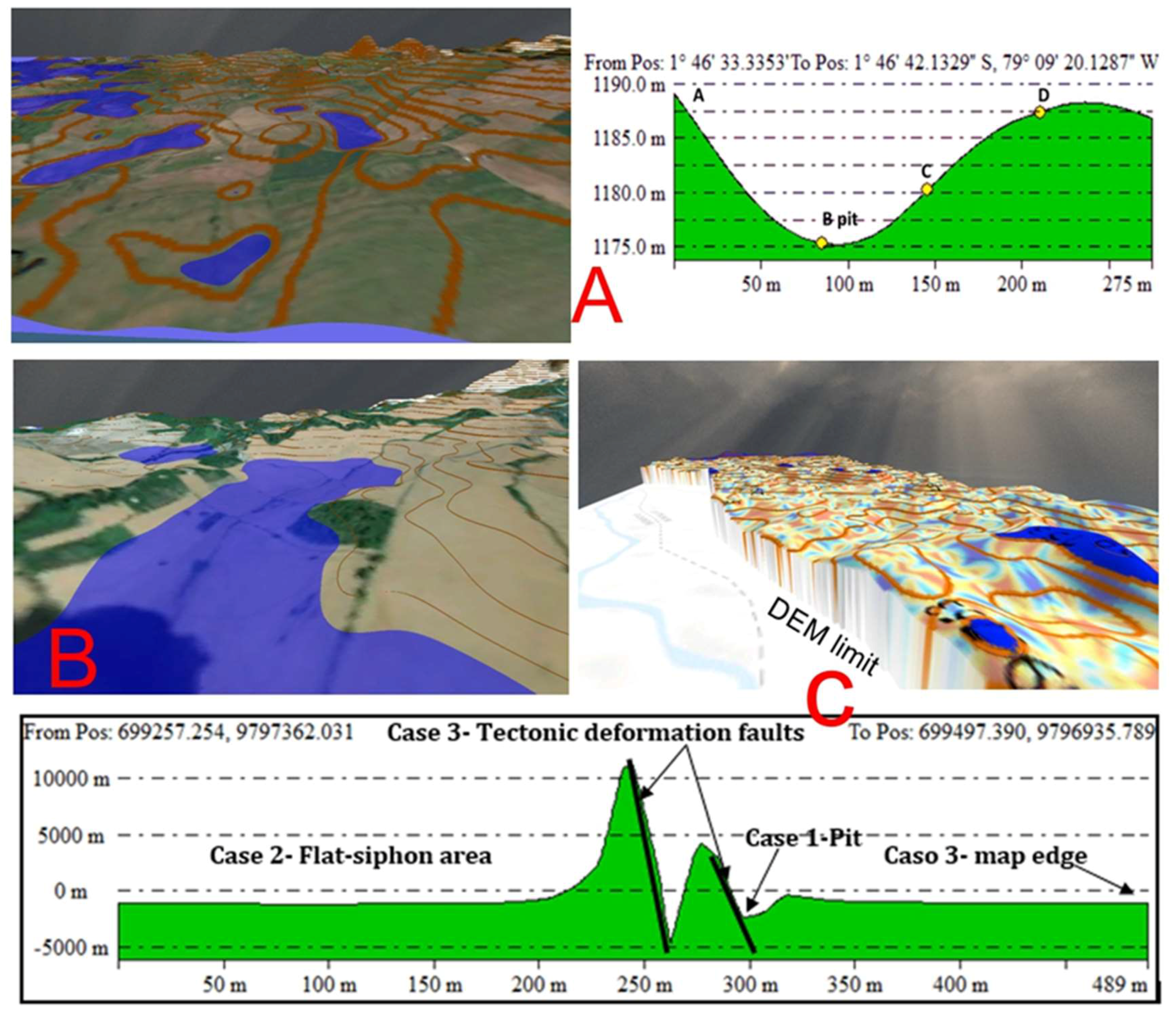
Three cases are possible in the drawing of flow lines, flow patterns, or flow (Figure 4A–C). In Case 1, cell C1 is surrounded by 8 cells higher than it. In this case, Cell C0 is a "pit" in point B (Figure 4A). In Case 2, cell C1 is part of a group of cells with the same dimension that represents flat areas. In the event that the flat area is surrounded by higher cells, it is known as a sink (Figure 4B). In Case 3, more than one cell are adjacent to C1 with a slope equal to the maximum. This problem can be called an indeterminacy, and it occurs when C1 is on a coastal edge or DEM boundary. However, if the DEM has abrupt discontinuities or inflection zones, these "indeterminate edges" within the DEM can determine the presence of regional tectonic structural systems such as faults, fractures, and terrain deformations (Figure 4C).

In Phase 3, the propagation rule is applied. The cell with the maximum negative slope defines the cell that will change state. In our example, the cell is C8 = −89.28; therefore, C8 is the cell that will light up (yellow in Figure 3F), so that the path of the flow line grows on the matrix, and its length depends on the iterations necessary to reach some of the completion conditions, thus creating the system of flow paths. The process is repeated from the new cell state with a negative maximum slope in an iterative process throughout the study grid (Figure 5A1,A2).

The chosen point (maximum slope) was incorporated in the downstream flow line and used as a basis to return to Phase 2, with negative and positive lateral-flow transport zones, flow accumulation zones, and flat areas. In Figure 5B1, the center of cell C0 is the start of the flow lines. In Figure 5B2, the drawing of the flow "downstream" line is displayed; and in Figure 5B3, the final plot of the flow line upstream and downstream from the starting cell C0 is depicted. Figure 5C1,C2 demonstrate the concentration downstream of the runoff flows that form channels and drainage networks that collect the waters of the entire basin and pour them into a single river at the mouth of the basin.

In Phase 4, the plane and profile curvatures in the matrix of the slopes of Figure 3A are calculated with Equations (4)–(7) below [23]:

$$\mathrm{D}=\frac{\left[\frac{\mathrm{P}7+\mathrm{P}4}{2}-\mathrm{P}0\right]}{{\mathrm{d}}^2};\mathrm{E}=\frac{\left[\frac{\mathrm{P}1+\mathrm{P}7}{2}-\mathrm{P}0\right]}{{\mathrm{d}}^2};\mathrm{F}=\frac{\left[\frac{\mathrm{P}1+\mathrm{P}7}{2}-\mathrm{P}0\right]}{{\mathrm{d}}^2};$$

(4)

$$\mathrm{G}=\frac{\left(\mathrm{P}3-\mathrm{P}7\right)}{2\mathrm{d}};\mathrm{H}=\frac{\left(\mathrm{P}1-\mathrm{P}5\right)}{2\mathrm{d}}$$

(5)

$$\mathrm{Plan}\mathrm{Curvature}:\mathrm{PC}=\frac{2\left({\mathrm{DH}}^2+{\mathrm{EG}}^2-\mathrm{FGH}\right)}{{\mathrm{G}}^2+{\mathrm{H}}^2}$$

(6)

$$\mathrm{Profile}\mathrm{Curvature}:\mathrm{PLC}=\frac{2\left({\mathrm{DG}}^2+{\mathrm{EH}}^2+\mathrm{FGH}\right)}{{\mathrm{G}}^2+{\mathrm{H}}^2}$$

(7)

In Phase 4, the flat and profile curvatures are calculated, which are one of the factors that contributes to relief deformation and instability. These curvatures were extracted directly from the DEM, apart from aspect and slope. The layouts of the flat curvature (concavity degree/convexity along an isoline perpendicular to the slope profile) and the profile curvature (concavity degree/convexity of the slope profile) were selected due to their influence over the water content that is stored in the soil and is responsible for mass movements when intense precipitations occur. These traced curvatures, such as continuous isolines, brake slopes and orientation originating natural fractures processes [24].

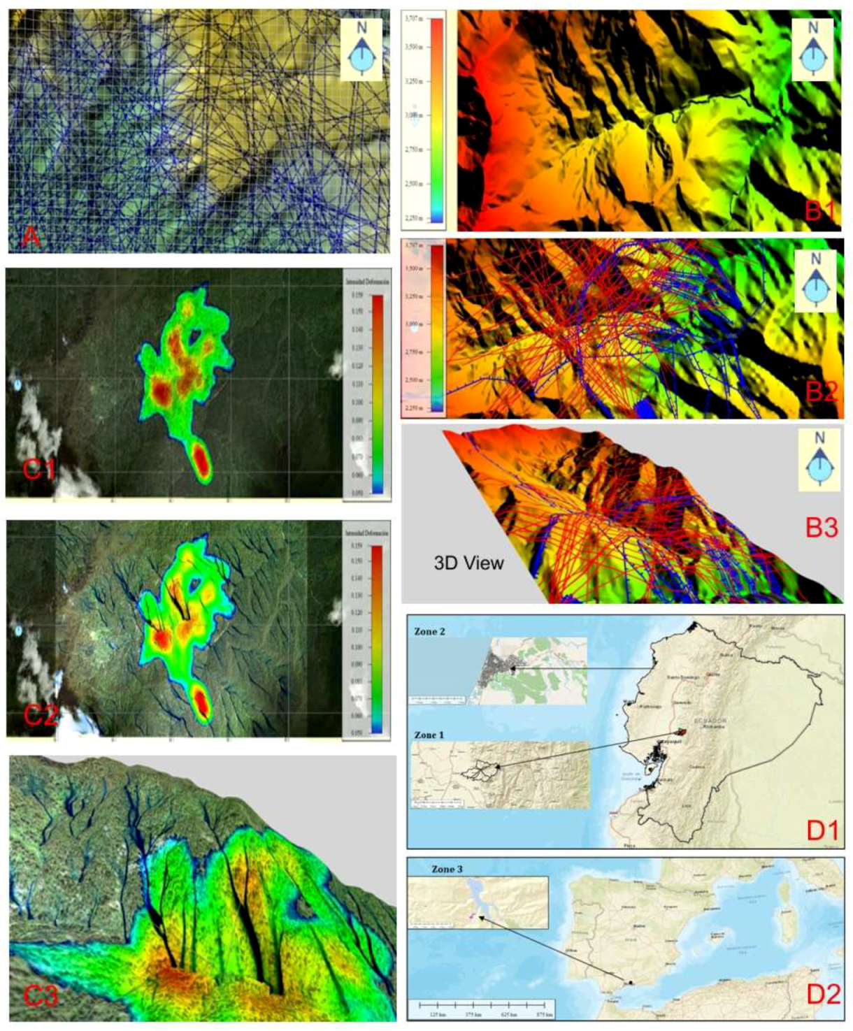
For the flat curvature, negative values show that the surface is concave upwards and positive values show that the surface is convex upwards. For the profile curvature, negative values show that the surface is convex upwards and positive values show that the surface if convex upwards. A cero-curvature value shows that the surface is flat for both types of curvature. Additionally, for each DEM cell, from the C0 cell, if the line that represents flow direction or curvatures is infinitely grown until the DEM edge is located, the structural lineaments (parallel lines to the curvatures) can be found, and deformation zones of the topographic relief in the intersections of these lines with the runoff flow paths from superficial water can be also found. The intensity of these concentrations values the deformation and susceptibility degree to mass movements in the study area. The curvature values are calculated in all cells of the DEM and intermediate meshes of slope change are drawn, obtaining the curvature vector (inflection that indicates concavity or convexity from node to node in degrees. Through this second operation, continuous facets of similar orientation within the DEM are connected via a direction vector from the cell centers. Vectors are where surface runoff water enters from the upper parts and erodes the deformed and weathered geoforms (morphological break line) (Figure 6A).

Within the digital elevation model, when the runoff and rupture lines were concentrated, erosion channels and areas of subsidence and breakage of the geoform were generated. Climate and topographic relief influence the pattern of a network, but the underlying geological structure is usually the most influential factor for the generation of this type of line and erosive processes. Hydrographic patterns are closely related to geology, which can help identify faults and structural lineaments [23,25,26,27].

The final active surface deformation of a region (for example, any DEM) with internal mass flows, can be spatially determined by the intersection of a set of morphological break lines that define critical points and regions of movement susceptibility (Figure 6B1–6B3). By applying a density filter to these lines, we obtained Morphological Sliding Plates (Figure 6C1–6C3), which relate morphology and geological structures, within which can be found fault escarpments, triangular facets of erosion, closing hills, pressure hills, deformation of alluvial cones, inversions of river beds, and other morphotectonic aspects associated with types of mass movements, such as rotational, translational, lateral expansion, falling blocks, flows in general, solifluction, and creep.

This methodology was validated in two areas of Ecuador (Figure 6D1) and one in Spain (Figure 6D2). Zone 1 is located between the towns of El Cadial, Chilcaloma, and Angas in the province of Bolívar, Ecuador. Zone 2 is located in the town of Pedernales, province of Manabí [28], Ecuador, and Zone 3 is in Arenas Del Rey in Granada, Andalusia, Spain [29].

3. Results

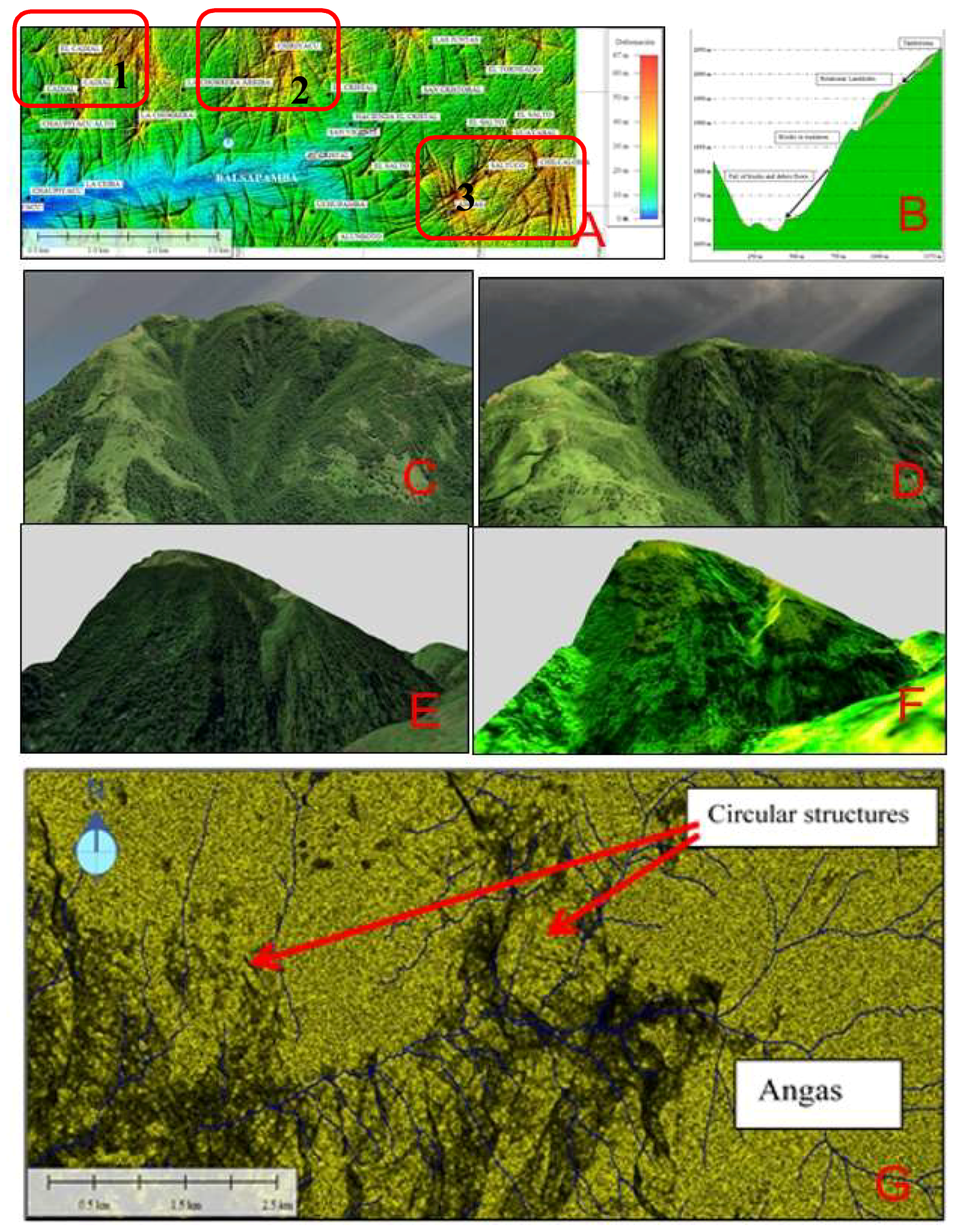
Zone 1: in all of Zone 1, structural guidelines, fractures, surface deformations and their type of associated mass movements, verified with field work, were found in three great plates of intense deformation, framed in red-colored polygons, (Figure 7A). Zone 1 in El Cadial–La Chorrera–La Chorrera de Arriba (340 ha); Zone 2 in Chiriyacu (262 ha); and Zone 3 in Agas–Saltuco–Chilcaloma–El Salto (370 ha). Besides that, other smaller deformation plates were found in Las Juntas and Santa Lucia. The lower zones of the river valleys, such as in Balzapamba, with an intense deformation with blue tendencies, represent mass-flow areas that generally affect these zones during intense precipitation times. For this zone, the digital elevation model of 10 m of spatial resolution was enough to obtain in detail the surface-relief deformations, structural lineaments and their relation with mass flow such as debris flow in ravines, eroded hillsides, and translational landslides (Figure 7B).

In Figure 7C–F, real photographs of the deformed hillsides were compared, without the application of the methodology proposed in Figure 7C,E, and with the application of the methodology proposed in Figure 7D,F, where intense deformations were obtained in these hillsides and their mass-movement systems associated with translational landslides, falling blocks, and mass flows. It also allowed for better comprehension of the relation between deformation of the topographic relief, mass movements, and the vulnerability of the population and its agroproductive systems to this kind of threat. An important characteristic of the obtained result with 10 m of spatial resolution is that the hidden geomorphological characteristics can be discovered as circular structures that can apparently be collapsed volcanoes, ancient megalandslides, and surface fractures caused by the location of intrusive locks (intrusive of Balsapamba). This circular structure, to the east of the Angas, is shown in a series of mass flows (Figure 7G).

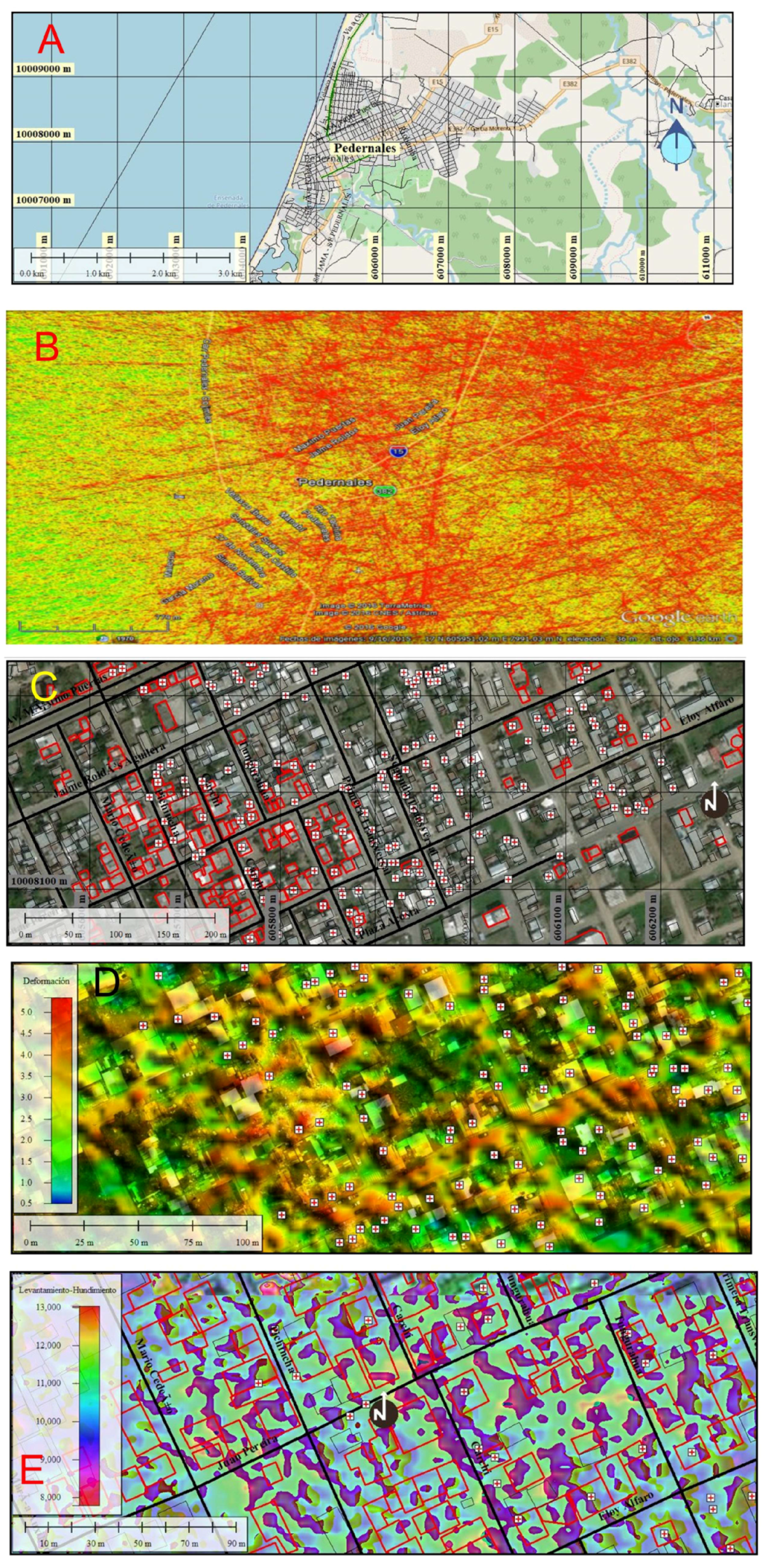
Zone 2: This zone is located on the town of Pedernales, province of Manabi, in the Ecuadorean coast. Pedernales’ population was the most affected by being near the epicenter of the earthquake of April 16, 2016, with a 7.8 score on the Richter Scale (Figure 8A). In Figure 8B we can observe the intensity of the concentration of structural geological lineaments and fractures (red-colored stripes) in the Zero Zone of Pedernales, obtained with a 3 m spatial resolution DEM before the earthquake. In the Zero Zone, the population suffered major destruction and building loss, as well as the loss of human lives (more than 183). In Figure 8C, we can observe destroyed buildings by the earthquakes, delimited by red-colored polygons. In Figure 8D, a detail of the structural lineaments that possibly amplified the superficial Rayleigh waves that destroyed houses and civil infrastructure is shown. In Figure 8E, we can observe a detail of the destroyed or severely damaged houses, marked with a red-colored cross and revised in the field after the earthquake. This infrastructure was raised (tendency to the yellowish-red color) or lowered (tendency to a violet-red color) as it is shown in the topographic relief image, obtained with an HSV saturation filter (saturation matrix). These houses were found near or on top of structural lineaments, surface fractures, and deformed zones obtained with the presented methodology. The houses with green colors show no destruction or cracks.

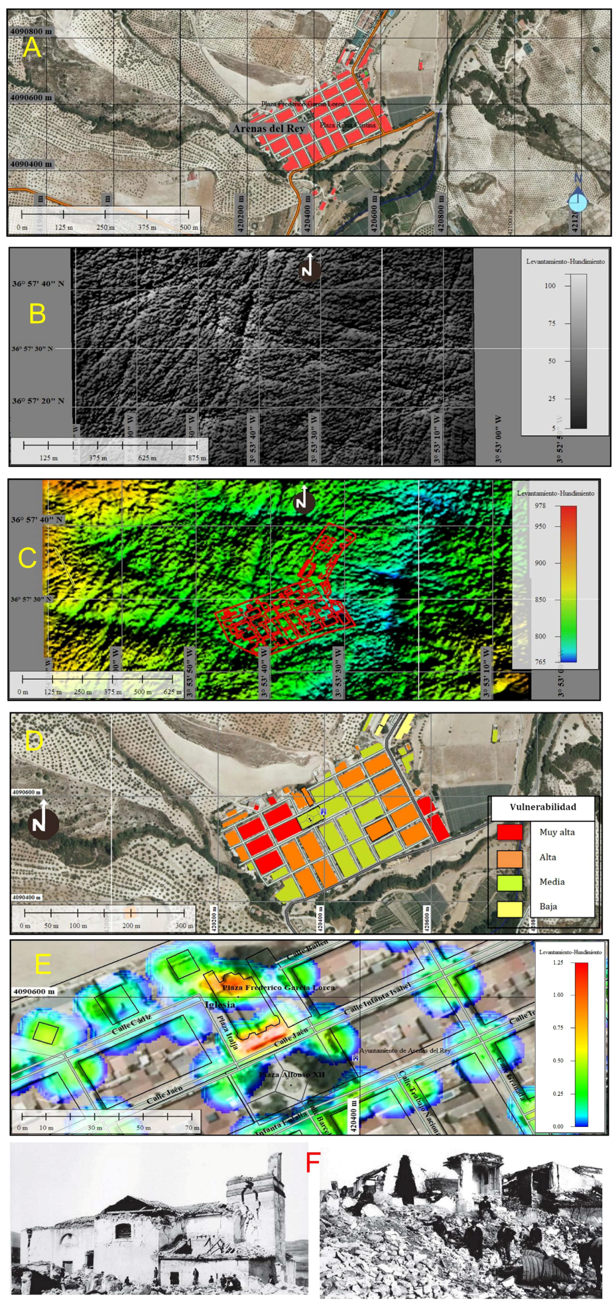
Zone 3: The third zone that theoretically validated this proposed methodology without field-work verification was in Arenas del Rey, Granada, Andalusia, España (Figure 9A). According to the chroniclers of the time, it was moved by an earthquake occurring on 25 December 1884, with its epicenter in Arenas del Rey, and a magnitude between 6.2 and 6.5 points in the Richter Scale, lasting for approximately 20 seconds, with a hypocenter between 40 and 50 km underground, causing between 1050 and 1200 deaths and approximately double that number in injuries. A total of 90% of civil structures were destroyed. Figure 9B and 9C shows surface structural geological lineaments that exist today in Arenas del Rey obtained using only the proposed methodology. Figure 9C shows the limits of the city (solid red-colored lines) and its location on top or near geological structural lineaments, with NS, NE–SW, and NW–SE directions, and surface fractures that possibly amplified the seismic waves of the 1884 earthquake and destroyed the city. This situation puts the population at high risk. Figure 9D shows the zoning of the seismic vulnerability of city plots in function of the actual terrain deformations that could raise or lower civil structures with a similar earthquake to the 1884 one. Figure 9E shows the concentrations (tendency to red color) of the lineaments and structural fractures in the Federico Garcia Lorca church, Alfonso XII plaza, and Jaen and Infanta Eulalia streets, which are one unified deformation train. These old deformations were possibly activated with the 1884 earthquake and destroyed the church, plazas, and other nearby buildings (90% of the population was killed). In the attached images (Figure 9F) of the document "The Earthquake of Alhama of Granada of 1884 and its Impact", the destruction of the church and the houses near the Alfonso XII plaza are represented. This evidence corroborates the actual deformation of those plots that place these buildings in danger.

4. Discussion

This standardized methodology by the SNGR, using heuristic and variable weighing to elaborate susceptibility to mass-movement maps, doesn’t identify geological structural lineaments, morphological ruptures lines, fractures, and surface-relief deformations. It also does not identify different types of mass movements, subsidence, and specific subsidence in small areas. However, these maps are a base reference to incorporate in them the geomorphologic traces mentioned, obtained with the proposed methodology that uses flow directions and its vector line with magnitude and the direction it represents. It also traces morphologic rupture lines using slope values, orientation of the slope, and flat and longitudinal curvatures, in public-license software such as SAGA and Arcview, and in commercial software such as Surfer and Rockworks 7 used in this study. This geomorphological traces were obtained in a quick fashion, unlike with the heuristic methodology, weighted variables, and analog methodologies such as the Mora Varhson image analysis that need larger thematic coverage and a larger amount of time for their processing.

Digital elevation models of 10 m, 3 m, and 5 m of spatial resolution used were enough to obtain relief-deformation zones based on structural lineaments and relief fractures. These deformation zones possibly contain weak geomechanic characteristics, can weather easily, and generate mass movements by rain such as in Zone 1, or by earthquakes with more than 6 points in the Richter Scale, such as the ones that shook the Ecuadorean coastline (2016) and Arenas del Rey, Andalucia, Spain (1884).

This methodology can be used with DEM of different spatial resolutions with ranges from 1 m (Lidar) up to big resolutions obtained from SRTM, AsterGdem, ALOS-PALSAR, Open Topography, and GTOPO 30, among other servers.

The ease to obtain digital elevation models with their public application allowed for quick obtaining of results to delimit borders, instability borders, and safe areas that can be used to locate meeting points, space routes, and safe areas to mobilize the population in the event of this type of threat. The application of this methodology can strengthen the operation of early warning systems to this type of threat.

5. Conclusions

The zoning of susceptibility by mass movements based on flow directions with the basic D8 Hydrological Method uses digital elevation models processed in free and commercial software, facilitating the identification and quick localization of structural geological lineaments, fractures, relief-deformation areas, and different types of mass movements.

A special characteristic of the presented methodology to obtain structural lineaments, fractures, and surface-relief deformations is that, depending on the digital elevation model resolution, it is possible to extract hidden geomorphologic characteristics such as extinct volcanic calderas, relief deformation by intrusive rocks and fractured pressure mounts, and deformed hillsides, among other geomorphologic traits.

The location of deformed areas by concentration of structural lineaments and relief fractures obtained from this methodology, with the field verification done in Ecuador (300 field control points) and in the base of chroniclers in Spain, have corroborated what happened in the areas of study.

Finally we conclude that the proposed methodology, unlike the standardized and analog methods, is economic, with a high precision degree, and can be applied to any geographic region before a disaster occurs caused by natural risks, such as intense rains or earthquakes with a ranking higher than 6 on the Richter scale. Thus, this methodology can be used as a forecasting mechanism through which maps of structural lineaments, fractures, and quaternary deformations with their own associated mass-movement types can be created, so populations located on or near these geomorphologic traits can be evaluated by their vulnerability degree to subsidence, structural collapse, landslides, and other types of mass movements. This will allow the elaboration of prevision and reduction maps to this type of risk in very high susceptibility zones and will strengthen municipal planning of the territory as well as its risk-management units, improving response and reduction protocols.

References

- Moore, I.D.; Grayson, R.B.; Ladson, A.R. Digital terrain modelling: A review of hydrological, geomorphological, and biological applications. Hydrol. Process. 1991, 5, 3–30. [Google Scholar] [CrossRef]
- Felicísimo, A.M. Digital terrain models: Introduction and applications in environmental sciences. Ph.D. Thesis, Universidad de Extremadura, Badajoz, Spain, 1994. [Google Scholar]
- Tarboton, D.G. A new method for the determination of flow directions and upslope areas in grid digital elevation models. Water Resour. Res. 1997, 33, 309–319. [Google Scholar] [CrossRef] [Green Version]
- Cando, M. Memories of the First International Symposium of Mass Movements. The Flow Paths of runoff as generators of mass movements. A vector approach Cuenca, Ecuador. Confidential report.
- Cando, M. MGE as Base of Support for the Construction of the Morphologic Breakage Model. In Proceedings of the Geospatial World 2002, Atlanta, GA, USA, 10–12 June 2002. [Google Scholar]
- Cando, M. Study of Landslides on the QuitoTena highway, the virgin stretch of Papallacta-Sardinas. In Proceedings of the International Symposium of Environmental Geology for the Planning of the use of the Territory, Puerto Varas, Chile, 2002. Memory of the Symposium. [Google Scholar]
- Cando, M. Tectonic Evidences and Simulation for a Potential Future Submarine Sector Collapse at Volcano Roca Redonda, Northern Galapagos and Ecuador 2007, 2nd ed.; Cuban Convention of Earth Sciences: La Habana, Cuba, 2007; Available online: http://catalogo.bnjm.cu/cgi-bin/koha/opac-detail.pl?biblionumber=96896 (accessed on 9 September 2018).
- Cando, M. The danger from flooding in the Lower Guayas River Basin 2010. Spanish Civil Guard: Memories of the VI National and IV International Conference on Nature and the Environment. Santander, Spain, 2010. Available online: http://jornadas.jabustillo.com/wp-content/uploads/2014/10/PROGRAMA-2010.pdf (accessed on 9 September 2018).
- Cando, M. Methodological development for the study of gravitational movements in hillsides: Application to the case of the Quito-Tena highway, section Papallacta-Baeza (Republic of Ecuador). Research proficiency in External Faculty of Sciences, Autonomous University of Madrid, Madrid, Spain, 2004. Confidential report.
- Cando, M. The Model of Morphological Break and its contribution in the prevention of mass movements. CIGMA 2004. Environmental Mining Geological Seminar, Cuenca, Ecuador. Unpublished report. 2004. [Google Scholar]
- Glaze, L.S.; Balogadem, S.M. DEM Flow Path Prediction Algorithm for Geologic Mass Movements. Environ. Eng. Geosci. 2003, 9, 225–240. [Google Scholar] [CrossRef]
- Kim, M.S.; Onda, Y.; Uchida, T.; Kim, K.J.; Song, S.Y. Effect of seepage on shallow landslides in consideration of changes in topography: Case study including an experimental sandy slope with artificial rainfall. Catena 2018, 161, 50–62. [Google Scholar] [CrossRef]
- Guinau Sellés, M.; Vilajosana Guillén, I.; Vilaplana, J.M. GIS-based debris flow source and runout susceptibility assessment from DEM data—A case study in NW Nicaragua. Nat. Hazards Earth Syst. Sci. 2007, 7, 703–716. [Google Scholar] [CrossRef]
- Han, S.; Yang, H.; Fan, T.; Xiao, D.; Moiwo, J.P. Precipitation-runoff processes in Shimen hillslope micro-catchment of Taihang Mountain, north China. Hydrol. Process. 2012, 26, 1332–1341. [Google Scholar] [CrossRef]
- Kim, K.S.; Song, Y.S. Geometrical and geotechnical characteristics of landslides in Korea under various geological conditions. J. Mount. Sci. 2015, 12, 1267–1280. [Google Scholar] [CrossRef]
- Lanni, C.; Borga, M.; Rigon, R.; Tarolli, P. Modelling shallow landslide susceptibility by means of a subsurface flow path connectivity index and estimates of soil depth spatial distribution. Hydrol. Earth Syst. Sci. 2012, 16, 3959–3971. [Google Scholar] [CrossRef] [Green Version]
- Bruning, J.N.; Gierke, J.S.; Maclean, A.L. An Approach to Lineament Analysis for Groundwater Exploration in Nicaragua. Photogramm. Eng. Remote Sens. 2011, 77, 509–519. [Google Scholar] [CrossRef]
- Brenning, A. Statistical geocomputing combining R and SAGA: The example of landslide susceptibility analysis with generalized additive models. Hambg. Beitr. Phys. Geogr. Landsch. 2008, 410, 23–32. [Google Scholar]
- Sárközynce, F. Introduction to GIS and Hydrologic modelling using ArcView 3.x. Available online: http://www.agt.bme.hu/public_e/ (accessed on 7 September 2018).
- Harrop, J. Rockworks version 7. Geological Software Collection, Rockware Inc., Golden, Colorado, US $495. Comput. Geosci. 1996, 22, 597–600. [Google Scholar] [CrossRef]
- Golden Software Surfer 12 User’s Guide. Chapter 12: Vector Maps. Available online: http://downloads.goldensoftware.com/guides/Surfer12_Users_Guide_Preview.pdf (accessed on 7 September 2018).
- Ahmad, T.; Sinha, K.; Chakraborty, P.P. GIS Surface Models and Terrain Analysis. RS and GIS XXVI. Available online: http://epgp.inflibnet.ac.in/epgpdata/uploads/epgp_content/S000448GO/P000602/M022483/ET/1505382131E-TextGISSurfaceModelsandTerrainAnalysis.pdf (accessed on 7 September 2018).
- Martínez-Graña, A.M.; Goy, J.L.; Zazo, C.; Yenes, M. Engineering Geology Maps for Planning and Management of Natural Parks: “Las Batuecas-Sierra de Francia” and “Quilamas” (Central Spanish System, Salamanca, Spain). Geosciences 2013, 3, 46–62. [Google Scholar] [CrossRef] [Green Version]
- Dai, F.C.; Lee, C.F. Landslide characteristics and slope instability modeling using GIS, Lantau Island, Hong Kong. Geomorphology 2002, 42, 213–228. [Google Scholar] [CrossRef]
- Silva, P.G.; López, M.; Roquero, E.; Huerta, P.; Martínez-Graña, A.M. Chronology of fluvial terrace sequences for Large Atlantic Rivers in the Iberian Peninsula (Upper Tagus and Duero drainage basins, Central Spain). Q. Sci. Rev. 2017, 166, 188–203. [Google Scholar] [CrossRef]
- Martínez-Graña, A.M.; Goy, J.L.; Zazo, C. Geomorphological applications for susceptibility mapping of landslides in natural parks. Environ. Eng. Manag. J. 2016, 15, 1–12. [Google Scholar] [CrossRef]
- Vidal Montes, R.; Martínez-Graña, A.M.; Martínez Catalán, J.R.; Ayarza, P.; Sánchez San Román, F.J. Vulnerability to groundwater contamination, SW Salamanca, Spain. J. Maps 2016, 12, 147–155. [Google Scholar] [CrossRef]
- Noji, E. Equador Struck by Magnitude 7.8 Earthquajke 16 April 2016. Available online: https://es.slideshare.net/enoji/16-april-2016-magnitude-78-earthquake-strikes-ecuador (accessed on 9 September 2018).
- Francisco, V.S. The Earthquake of Alhama de Granada of 1884 and its impact. Instituto Andaluz de Geofísica/Department de Física Teórica y del Cosmos, Universidad de Granada: Grananda, Spain, 2011. Available online: https://www.raco.cat/index.php/AnuariVerdaguer/article/viewFile/262467/349631 (accessed on 9 September 2018).
Figure 1.
Comparison of structural guidelines obtained with remote-sensing methodology and the proposed methodology applied to the same area (Nicaragua) with the same 20 m spatial resolution digital elevation model. (A) Results of the coincidence between the lineaments obtained by remote sensing with stereoscopy. (B) Structural guidelines obtained with the proposed method. (C) Coincidences and advantages of the proposed methodology. (D) Deformed relief.
Figure 2.
Process followed for the extraction of surface runoff flows from precipitation water in the D8 hydrological model.
Figure 3.
(A) Assignment of cells (C0–C8) and heights of the terrain (Z0–Z8) for the calculation of slopes (P0–P8) according to Model D8. (B) Determination of the Maximum Pending Line AB. Point A is the starting point on the 200 m level curve. Points B, C, and D define segments AB, AC, and AD, respectively. The line of the maximum slope corresponds to the shortest AB segment, which is generally the route through which water flows from the highest point A. (C) Tracing of the maximum-slope line in a digital elevation model and tracing of the maximum-slope line in a digital elevation model (DEM). (D) Initial point of the line at time t = 0, with initial state C0 = 1, and dimension assigned by the DEM = 1068.44. (E) Initial cell at the elevation of 1068.44 meter above sea level (masl) for the generation of flow lines of meteoric water-surface runoff according to the D8 Model and (F) final score.
Figure 4.
(A) Case 1, pit: cell C1 is surrounded by 8 cells higher than it. (B) Case 2: Cell C1 is part of a group of cells with the same dimension, which represent flat areas. If the flat area is surrounded by higher cells, it is as a sink. (C) Case 3, Indeterminacy: more than one cell is adjacent to C1 with slope equal to the maximum. This problem is called an indeterminacy and occurs when C1 is not on a coastal edge or DEM boundary.
Figure 5.
(A1, A2) Operation of the propagation rule. The cell with the maximum negative slope is the cell that will change status from 0 (off) to 1 (on) as shown in yellow. (B1) The center of cell C0 is the start of the drawing of the flow lines. (B2) Drawing the flow line “downstream”. (B3) The final plot of the flow line upstream and downstream from starting cell C0. (C1) Plotting the flow lines of surface-water runoff from the elevation mesh of the DEM and (C2) concentration in drainage channels and erosion of geoforms.
Figure 6.
(A) Phase 4: Tracing of curvature vectors created by the trace of intermediate meshes of change in slope and inflection that indicates concavity or convexity surfaces. (B1) Final state of active surface deformation of a region. (B2 and B3) with internal mass flows determined by the intersection of a set of morphological break lines (blue lines-morphological rupture and red lines-runoff flows) that define critical points and regions of susceptibility to movement. (C) Formation of the Morphological Sliding Plates in a function of flow lines and rupture lines. (C1) Sliding mantles without internal flow, (C2) sliding mantles with internal flows, and (C3) 3D model with sliding mantles obtained. (D) Study areas. Zone 1 (D1): Located between the towns of El Cadial, Chilcaloma, and Angas, in the province of Bolivar, Ecuador. Zone 2 (D1): Town of Pedernales, province of Manabí, Ecuador. Zone 3 (D2): Arenas Del Rey in Granada, Andalusia, Spain.
Figure 7.
Zone 1: Located between the towns of El Cadial, Chilcaloma, and Angas, in the province of Bolívar. There are three morphological deformation plates. (A1) El Cadial-La Chorrera–La Chorrera de Arriba (340 ha), (A2) Chiriyacu (262 ha), (A3) Angas–Saltuco–Chilcaloma–El Salto (370 ha). In these areas, the mountains are possibly fractured by the Balzapamba Intrusive. (B). Detail the surface-relief deformations and structural lineaments. (C, D, E, F) Field check of the geoforms with real images without and with the application of the proposed methodology at scale 1/10,000. The response of the model was evidence in more than 300 control points. (G) Circular structures obtained with the proposed methodology of hidden geomorphological traits.
Figure 8.
(A) Location of Zone 2 in Pedernales. (B) Structural lineaments obtained with the proposed methodology. (C) Orthophoto with the destroyed homes (red polygons) after the earthquake of 2016. (D) Location of the collapsed houses on top of the obtained structural lineaments. (E) Color-intensity filter and collapsed houses (red color).
Figure 9.
(A) Location of Zone 3 in Arenas del Rey, Granada, Andalusia, Spain. (B) Structural lineaments of the study area. (C) Positioning of the city outline on relief structural lineaments. (D) Vulnerability intensity by relief deformation in the city outline. (E) Punctual deformation in the Federico Garcia Lorca Church to Jaen Street. (F) Images of the 6.2 to 6.5 in the Richter scale earthquake in 1884.
© 2018 by the authors. Licensee MDPI, Basel, Switzerland. This article is an open access article distributed under the terms and conditions of the Creative Commons Attribution (CC BY) license (http://creativecommons.org/licenses/by/4.0/).
Share and Cite
MDPI and ACS Style
Cando Jácome, M.; Martínez-Graña, A. Numerical Modeling of Flow Patterns Applied to Analysis of Susceptibility to Movements of the Ground. Geosciences 2018, 8, 340. https://doi.org/10.3390/geosciences8090340
AMA Style
Cando Jácome M, Martínez-Graña A. Numerical Modeling of Flow Patterns Applied to Analysis of Susceptibility to Movements of the Ground. Geosciences. 2018; 8(9):340. https://doi.org/10.3390/geosciences8090340
Chicago/Turabian StyleCando Jácome, Marcelo, and Antonio Martínez-Graña. 2018. "Numerical Modeling of Flow Patterns Applied to Analysis of Susceptibility to Movements of the Ground" Geosciences 8, no. 9: 340. https://doi.org/10.3390/geosciences8090340
Note that from the first issue of 2016, this journal uses article numbers instead of page numbers. See further details here.