Kriging with a Small Number of Data Points Supported by Jack-Knifing, a Case Study in the Sava Depression (Northern Croatia)

Abstract

The semivariogram and the ordinary kriging analyses of porosity data from the Sava Depression (Northern Croatia), are presented relative to the Croatian part of the Pannonian Basin system. The data are taken from hydrocarbon reservoirs of the Lower Pontian (Upper Miocene) age, which belong to the Kloštar Ivanić Formation. The original datasets had been jack-knifed with the purpose of re-sampling and calculating the more reliable semivariograms. The results showed that such improvements can assist in the interpolation of more reliable maps. Both sets, made by the original and re-sampled data, need to be compared using geological recognition of isoline’s shapes (such as “bull-eye” or “butterfly” effects) as well as cross-validation results. This comparison made it possible to select the most appropriate porosity interpolation.

1. Introduction

The hydrocarbon reservoirs in the Sava Depression (Northern Croatia) are in the secondary or tertiary recovery phase. Most are supported by water injection. Two fields from the abovementioned depression with still significant production of hydrocarbons from selected reservoirs are analyzed here. These are field “A”, reservoir “L”, and field “B”, reservoir “K”, hydrodynamic unit “K1”.

The analysis in the continuation is based on many previous works published for the Sava Depression as well as the entire Croatian part of the Pannonian Basin System (CPBS). Statistical data and mapping of previous regional works are represented in continuation, especially in the Sava Depression. Hence, Malvić [1] presents the use of descriptive statistics (porosity vs. depth) and tests (t-, F-tests) and the Pearson correlation for the interpretation of the influence of increasing depth on the decrease of porosity in the Bjelovar Sub-depression (the Kloštar Ivanić Formation, Pepelana and Poljana Members). The author of [2] identified the kriging method as the most appropriate method for porosity interpolation in the Sava Depression, based on the mapping results done in the Sava Depression sandstones and cross-validation results. For the first time in Croatian geology, [3] applied jack-knifing in the variogram modelling of the reservoir variables for data from the Stari Gradac-Barcs Nygat Field (the Drava Depression). In the same field, [4] applied stochastically improved probability of success calculation for the first time. Reference [5] described the most often applied kriging techniques—simple, ordinary and indicator—and provided the optimal Lagrange value in the ordinary kriging method for the CPBS. Reference [6] gave sequential Gaussian simulation (SGS) results for the Kloštar Field in the Sava Depression. Reference [7] described the criteria for choosing between kriging, co-kriging and simulations using examples from the CPBS. Reference [8] analyzed lithofacies from logs, porosity maps, and made indicator transformation and maps (the Kloštar Field, Sava Depression). In the same field, [9] analyzed reservoir porosity, depth and thickness using 100 realizations of the SGS. Reference [10] applied geostatistics for the most detailed geological model of the Kloštar Field and typical depositional model of the Upper Miocene sandstone reservoirs in the Sava Depression. Reference [11] described the four main applications of geostatistics and recommended for the CPBS such interpolation for the datasets with 20 or more points. Reference [12] pointed out that ordinary kriging was the most often geostatistical technique applied for mapping of the sandstone reservoirs in the Sava Depression. Reference [13] applied the sequential indicator simulations for porosity mapping (of the CPBS), using reservoir thickness maps as the secondary source of information. Reference [14] applied a stochastically improved probability model of geological risk as a new approach to the clastic reservoirs in the CPBS. Reference [15] used ordinary and indicator kriging, as well as SGS, for CO₂ sequestration in oil reservoirs. Deterministic methods for geological risk have been adapted for sequestration purpose. Reference [16] mapped the Bjelovar Sub-depression using ordinary kriging and a digitalized set of older maps. Reference [17] analyzed data from the Šandrovac Field (the Drava Depression) comparing ordinary kriging, inverse distance weighting and nearest neighborhood. Reference [18] used universal kriging for the first time in the Bjelovar Sub-depression and proved it the best interpolation method in the CPBS if a regional trend is visible. Reference [19] described the application of stochastic simulation for the Lower Pontian reservoir in general (the CBPS). Reference [20] presented the problem of the selection of an appropriate mapping method for a dataset with a small number of data (i.e., nearest neighborhood vs. inverse distance weighting).

Regarding the geostatistical theory, there are a large number of available papers and books where the theory and/or its application had been presented in a clear manner. We decided to select several works where the review of the variogram calculations and kriging algorithms had been presented. Thus, [21] proposed a two-step procedure for variogram interpretations in hydrocarbon reservoir modelling, i.e., for modelling spatial variability of variables, such as lithofacies, porosity, etc. The emphasis was given to total variance of the analyzed variable(s), divided into variance regions. The same authors [22] stated the strong connection between the reliable variogram model and depositional model, i.e., the continuity of geological features. It is especially important in the case of geological anisotropies as a reflection of the depositional environment.

Kriging techniques are numerous, and all are developed as variations of simple kriging. For example, [23] presented the application of the sequential indicator simulation algorithm with the goal to obtain a set of equiprobable realizations. They used a conditional variant, respecting the data and simulating other cells. The intention was to show the heterogeneity in the Berea Sandstone reservoir. An interesting application of the secondary variable in kriging matrices has been presented [24] using the collocated co-kriging approach in defining hydrocarbon reservoirs, i.e., to mapping the top of stratum. They correlated wells with the seismic data, and compared kriging with external drift and co-kriging, where both use secondary information as drift or additional variable. Recently, [25] presented a method for connecting porosities from cores and logs for consequent modelling of permeability. Ordinary kriging and co-kriging was applied on the multi-facies, shale and sandstone datasets (South Rumaila Field, Southern Iraq). The permeability had been estimated using porosity data and algorithms of ordinary kriging. Then, the cross-variogram analysis was done to model core permeability (primary) using core porosity (secondary variable), and both are functions of logged values (neutron porosity, water saturation, and their depth). The results had been checked using cross-validation and visual observation of the predicted and observed values. The co-kriging algorithm obtained better results. In addition, [26] applied Bayesian kriging for spatial prediction of the permeability in the hydrocarbon reservoir. All previously applied “conventional” kriging techniques did not correctly estimate the uncertainty in the co-variance structure, so Bayesian kriging was selected with the purpose of taking prior knowledge of the data, such as expert opinions. The uncertainty is given in the form of a posterior probability, and unbiased estimation led to a more realistic view of the reservoir (the small unrealistic “regions” are eliminated). The model had been applied in the sandstone of the tidal depositional environment (the South Rumaila Field), even using the Bayesian approach for stochastic simulations and selection of the P10, P50 and P90 realizations.

Two famous resampling techniques are jack-knifing and bootstrapping. Both are previously used in different geological analysis, especially those of hydrocarbon reservoirs. Reference [27] presented multi-plausible (probable) variograms, where the uncertainty is addressed to each point (lag). They can be basically used for one or more, equally probable, kriging realizations. Multiple plausible variograms may be fitted knowing the uncertainty at each variogram point, 2γ (h). Multiple geostatistical realizations may then be constructed and subjected to process assessment in order to measure the impact of this uncertainty. Theoretically, if all random variables are independent, the Gaussian distribution could be applied, and although it is not the case in reservoir dataset(s), such multi-Gaussianity simplifies the calculation and is mostly acceptable. Authors made several local simulations of four-point locations (so evaluated the 4^th-order moments) and eventually calculated the confidence interval for each variogram point (25, 50, 75 and 95%). Later, [28] presented a generalized bootstrap method for the analysis of semivariogram (i.e., covariance) uncertainties. As the semivariogram is based on measurements, bootstrap could be applied to increase knowledge about the reliability of calculated spatial continuity. Authors used several approaches and datasets, such as LU decomposition and non-Gaussian random field. The bootstrap percentile confidence intervals were not centered around the empirical semivariograms and did not use distributional assumptions for their construction (vs. symmetrical intervals based on standard error, estimated from parametric equation or bootstrap).

All these works have been analyzed with the purpose of solving the problem of a relatively small number of data points, characteristic for almost each particular (and selected) structure in the Sava Depression. Hence, here we first describe two such typical structures in the depression, i.e., their lithostratigraphic parts where there are hydrocarbon reservoirs proven, where most of the available geological variables (petrophysical, saturation, granulometry, injected water) have been measured. This is followed by a relatively simple geostatistical analysis of the reservoir porosity, which is also assumed to have a normal distribution. Such a statement is given as axiomatic, due to an overly small number of hard data to test normality. Unfortunately, new data cannot be additionally collected (most due to expense), so the statistically available methods (jack-knifing) for increasing the number of calculations per each variogram lag and for the “similar datasets” has been tested.

1.1. Basic Equations of the Applied (Geo-)Statistical Techniques/Methods

Jack-knifing is a resampling statistical technique, later upgraded into, e.g., bootstrapping. It is useful for statistics estimation, sequentially leaving out each value from datasets and calculating the statistical parameters of remaining data. For example, if the estimated parameter is the population mean ($\overline{x}$), using jack-knifing it is possible to calculate the mean of each sub-dataset that includes all but the i-th measurement (${\overline{x}}_i$) using Equation (1):

$${\overline{x}}_i=\frac{1}{n-1}·{\displaystyle \sum _{j=1,j\ne i}^n}{x}_j,i=1\dots n$$

(1)

where ${\overline{x}}_i$: mean of sub-dataset, where i-th data is skipped, n: number of data points, j: data currently analyzed.

These n estimations of the mean also form the distribution that characterizes sample statistics with a mean equal to the average of ${\overline{x}}_i$.

Variogram (2γ) is the basic geostatistical tool for spatial analysis of a selected regionalized variable. This is defined as the difference between two values of a selected variable at distance h (Equation (2)):

$$2\gamma \left(h\right)={\left[z-z\left(h\right)\right]}^2$$

(2)

where 2γ(h): variogram calculated at distance h; z: value of variable in selected location; z(h): value of variable at distance h from selected location.

Once the experimental variogram is approximated with a theoretical function it can be calculated in the kriging equations only based on distances between two points (not from values). For the N data pairs at distance h (i.e., lag or class), the variogram is calculated from Equation (3):

$$2\gamma \left(h\right)=\frac{1}{N}·{\displaystyle \sum _{n=1}^{N\left(h\right)}}{\left[z-z\left(h\right)\right]}^2$$

(3)

where N: number of data pairs compared at distance h; z: value of variable in selected location; z(h): value of variable at distance h from selected location.

The simplest way to present linear estimation is given by Equation (4):

$$Z_k={\displaystyle \sum _{i=1}^n}{\lambda }_i·Z_i$$

(4)

where Z_k: values of regionalized variable at selected location (estimated from hard data); Z_i: known values at the location i (hard-data); λ_i: weighting coefficient for location i.

The values of Z_i are assumed to have a Gaussian distribution, especially if the number of samples is large (i.e., random variable with a large number of independent samples respects the central limit theorem). Weighting coefficients are calculated using a system of linear equations, such as the kriging matrices (e.g., [29,30,31]). The main advantages of kriging (vs. simpler mathematical methods) are a better consideration of the data anisotropy (by variogram analysis) and possible clustering. Moreover, the values of weighting coefficients in kriging depend on distance, not on values, thanks to the variogram model. This is why such a distance is sometimes known as the “statistical distance”. The matrix equitation of kriging is given here with an example of simple kriging (Equation (5)):

$$\left[\begin{array}{cccc}\gamma \left(Z_1-Z_1\right)& \gamma \left(Z_2-Z_2\right)& \cdots & \gamma \left(Z_1-Z_n\right)\\ \gamma \left(Z_2-Z_1\right)& \gamma \left(Z_2-Z_2\right)& \cdots & ⋮\\ ⋮& ⋮& \cdots & ⋮\\ \gamma \left(Z_n-Z_1\right)& \gamma \left(Z_n-Z_2\right)& \cdots & \gamma \left(Z_n-Z_n\right)\end{array}\right]·\left[\begin{array}{c}{\lambda }_1\\ {\lambda }_2\\ ⋮\\ {\lambda }_n\end{array}\right]=\left[\begin{array}{c}\gamma \left(x_1-x\right)\\ \gamma \left(x_2-x\right)\\ ⋮\\ \gamma \left(x_n-x\right)\end{array}\right]$$

(5)

where $\gamma \left(Z_1-Z_2\right)$: semivariogram values between values Z₁ and Z₂ (can be read from variogram curve); $\gamma \left(Z_n-Z_n\right)$: 0 (semivariogram cannot be calculated between the same values); $\gamma \left(x_n-x\right)$: semivariogram on distance between known value x_n and estimated value x. λ_n: weighting coefficient for location n.

Simple kriging is a basic technique, but is not unbiased estimation. All other kriging techniques have added some constraint in the equations and are described as BLUE (best linear unbiased estimator) techniques.

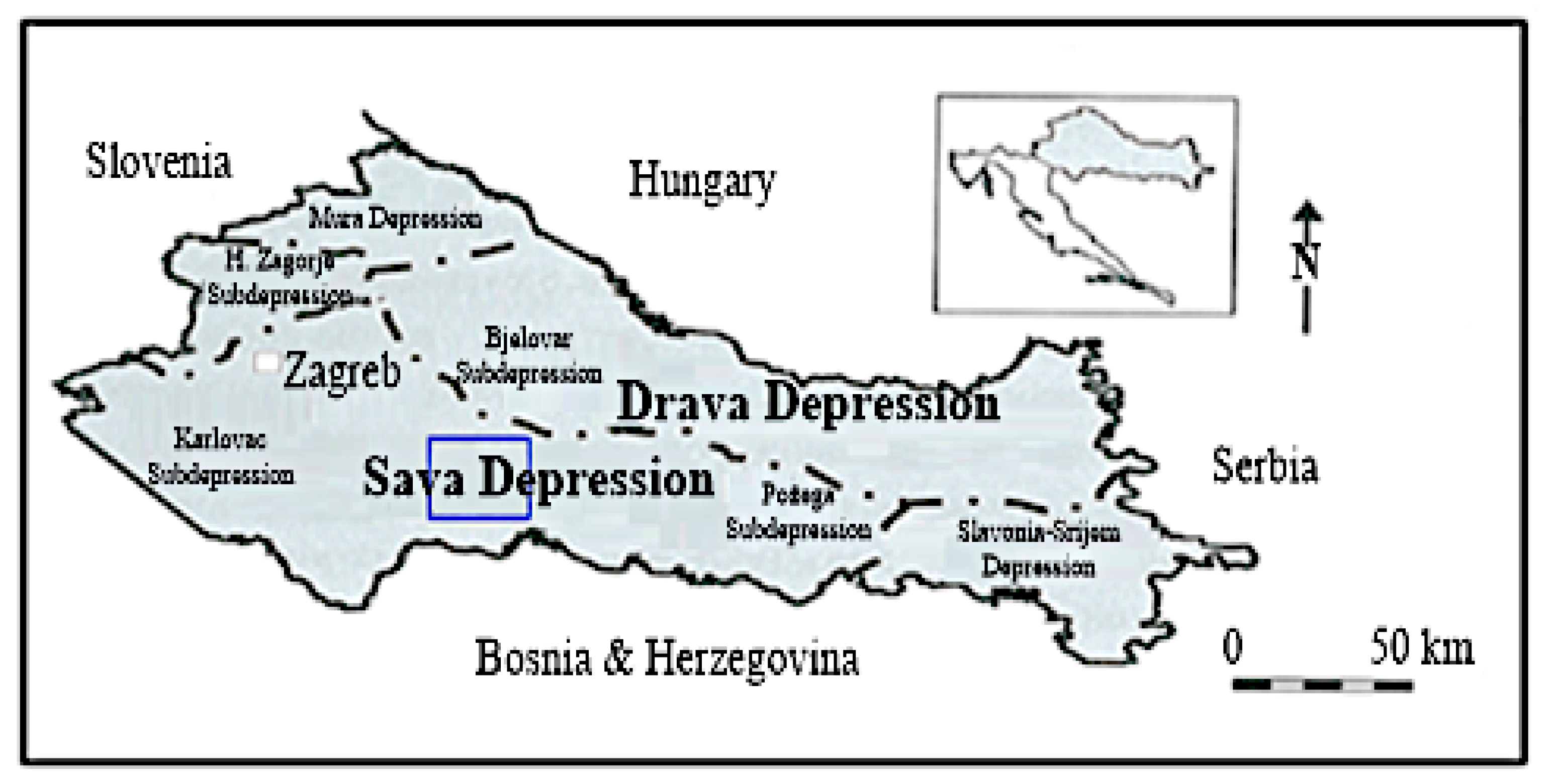
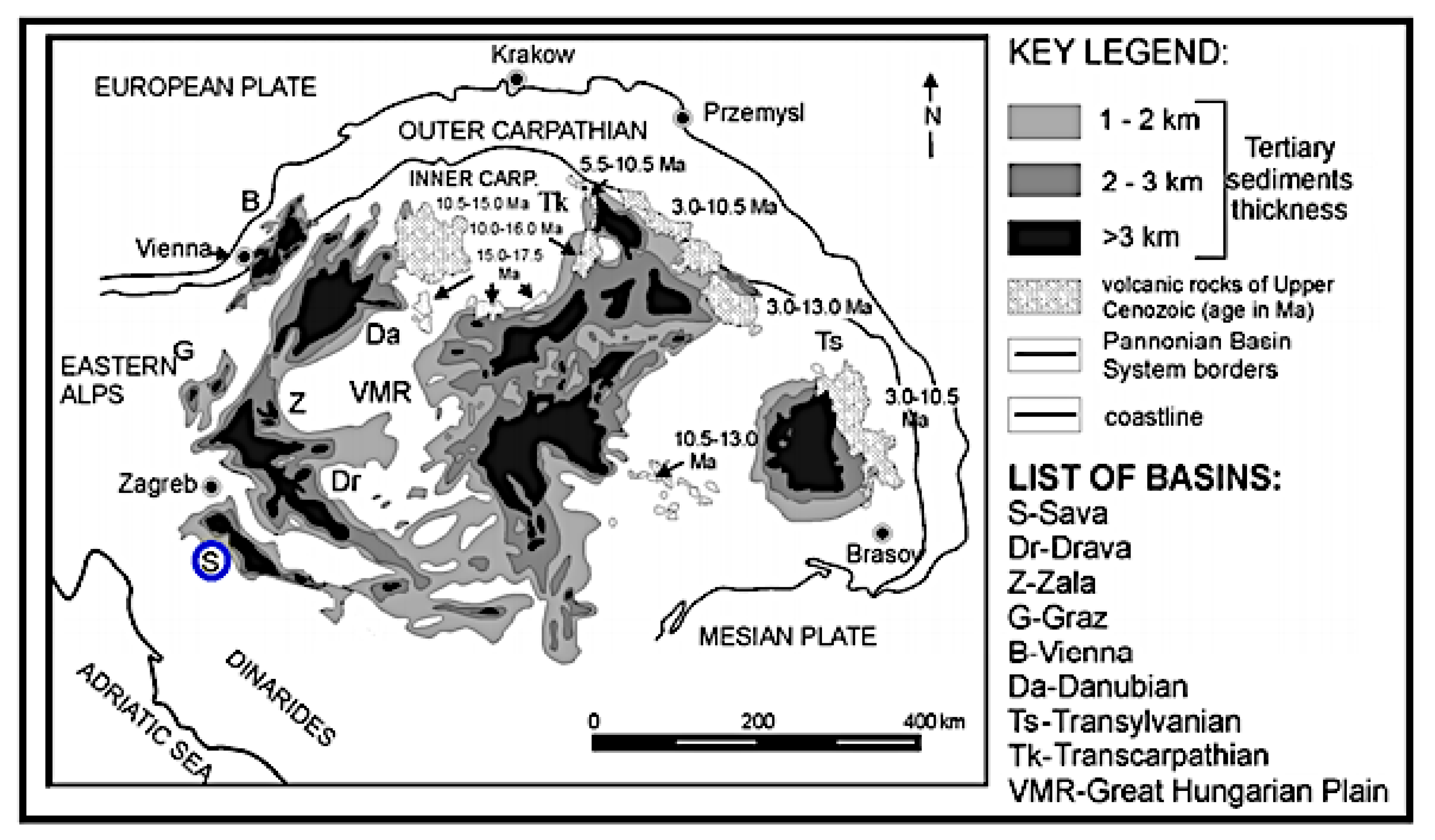
1.2. Geographical Locations of the Analyzed Hydrocarbon Fields (Northern Croatia)

For the fields “A” (reservoir “L”) and “B” (reservoir “K”/HD “K1”) two variables were collected (porosity, injected water) and mapped with several methods (nearest neighborhood, inverse distance weighting, kriging). Both fields are located in the Sava Depression, about 90 km south-east from the capital Zagreb (Figure 1) and close to the highway A3 (5 km) and regional railroad (4 km).

The smaller location maps of analyzed fields are presented at Figure 2 (the fields “A” and “B” with blue and red borders, respectively). Both fields are on hilly terrain. “A” is an elongated structure with strike NW–SE and altitude 113–216 m, crossed by numerous landslides, and partially forested. Similarly, the altitude of field “B” is 120–231 m. The hills are steep and locally forested.

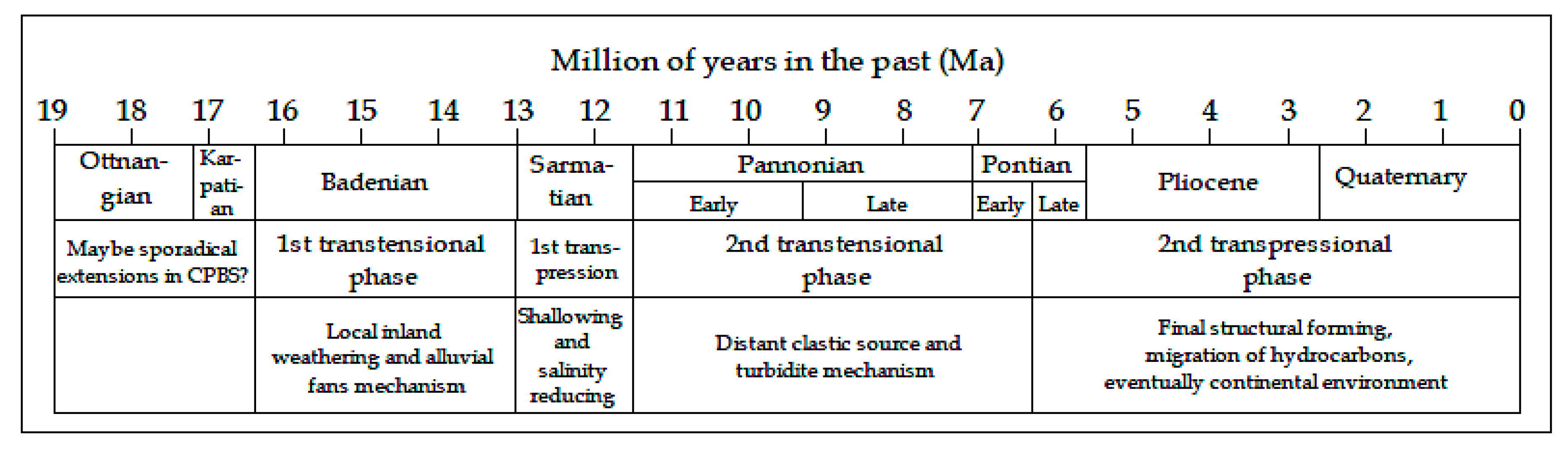
2. Geological History of the Western Part of the Sava Depression

The CPBS is located at the very south-western margin of the PBS. Its marginal location, regional position of the pre-Neogene basement and later tectonics caused structural elongation northwest—southeast. The entire CPBS is divided into four depressions—Sava, Drava, Mura and Slavonia-Srijem (Figure 1 and Figure 3).

The CPBS had been covered by shallow marine environments of the Paratethys during the Badenian and Sarmatian (16.4–11.5 Ma). It was reduced in the Pannonian Lake during the Lower Pannonian (11.5–9.3 Ma), and disintegrated during the Upper Pannonian (9.3–7.1 Ma) and Pontian (7.1–5.7 Ma) into several smaller lakes. The next, relatively short, phase of a single Slavonian Lake [35] happened during the Pliocene. From the Upper Romanian the entire CPBS has been covered with continental facies, which also lasts today (Holocene). The main stages of geological evolution in the CPBS are shown on Figure 4.

There are several characteristic lithofacies for the Sava Depression (as well as for the CPBS). Carbonates and coarse-grained clastics dominated in the Middle Miocene (Badenian—Sarmatian), i.e., had been deposited in the marine environments. The Upper Miocene (Lower Pannonian—Upper Pontian) is characterized by two clastic lithotypes—sandstones and marls. Both are deposited in the lacustrine environments [37]. The analyzed hydrocarbon reservoirs, in the Sava Depression, belong to that depositional phase (Figure 5), when huge volumes of sand and silt were transported by turbidites [33,36,37]. During “calm” periods, different carbonate-rich mud was deposited. Such alterations of clastic is typical for “high” and “low” energy environments and characteristic of the Upper Miocene for the entire CPBS [32].

About 95% of Upper Miocene sandstone reservoirs in the CPBS are of turbidite origin. They include several lithofacies. The central part of the structure is “pure” medium-grained sandstones, which are gradually changed into silty or clayey sandstones and siltstones on structural margins. Such heterogeneity determined secondary migration paths, recovery and production regime.

Both analyzed fields (“A” and “B”) are located in the western part of the Sava Depression (Figure 5). Present-day production is supported by water injection in the Lower Pontian reservoirs (Figure 6), lithostratigraphically belonging to the Kloštar Ivanić Formation, i.e., the Pepelana Member. The sandstone and marl sequences are determined from spontaneous potential and resistivity logs (Figure 7 and Figure 8). The marls are also isolator rocks for Lower Pontian reservoirs.

3. Results

Exploration drilling in the analyzed fields dates to the 1960’s. Consequently, several types of reservoir data are available.

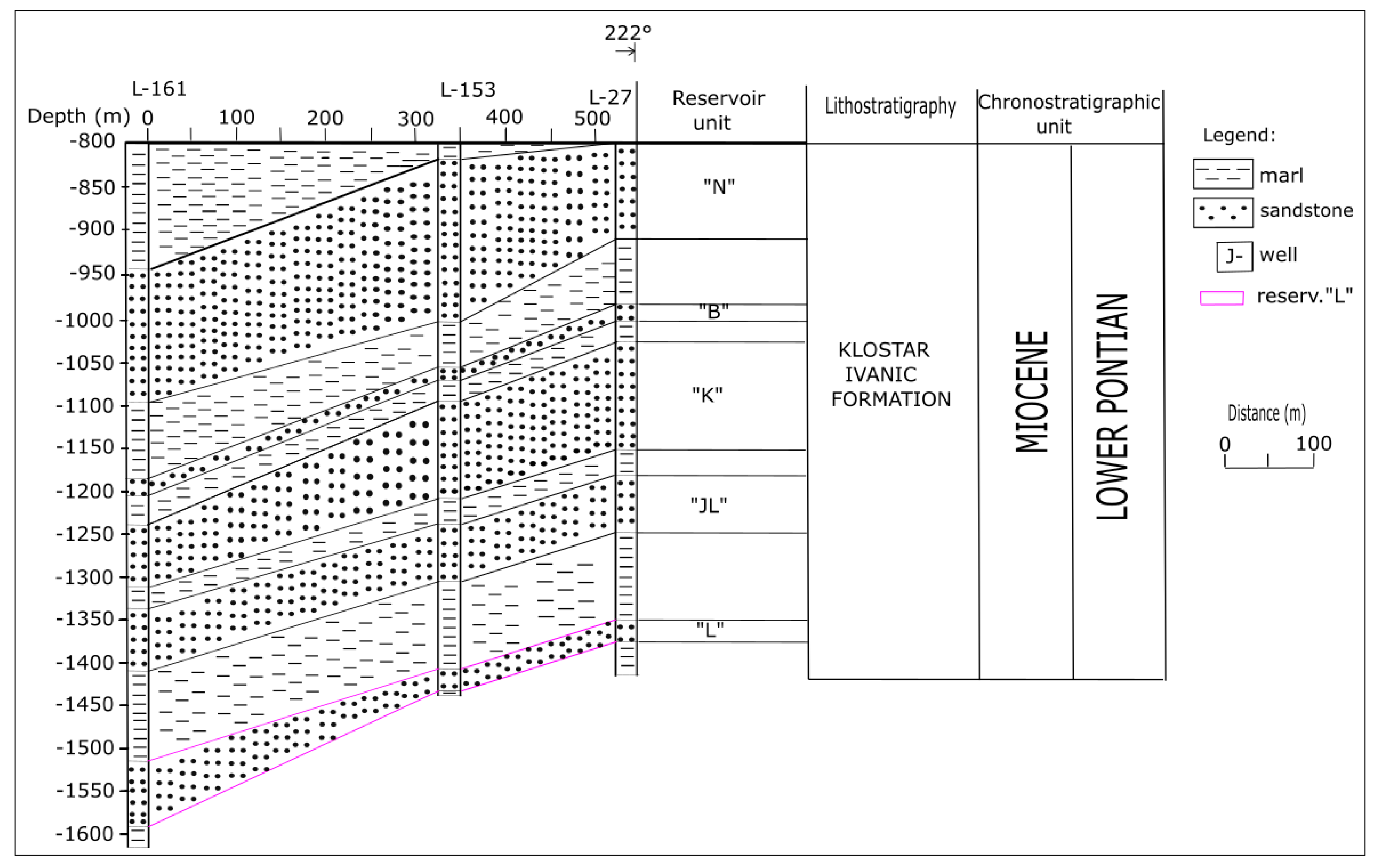
3.1. The Field “A”, Reservoir “L”

3.1.1. Reservoir Type

According to classification [38] the reservoirs in the field “A” are those of bedding type, capped by isolators, and margined with lithological and/or tectonic screens. The quartz dominated sandstones are enriched by mica. The reservoir sandstones are rhythmically interbedded with thin marls or sandy marls. The reservoir “L” is a single hydrodynamic unit.

3.1.2. Granulometry, Porosity, Saturation and Permeability of Sandstones

Granulometry has been calculated from cores and CaCO₃ using calcimetry analysis (

Table 1. Granulometry of reservoir “L” (M_d—mean grain diameter, S_o—coefficient of sorting, S_k—coefficient of asymmetry) (from archive of INA Plc.).

Well	Md	So	Sk	Sand (%)	Coarse Silt (%)	Clay (%)	CaCO3 with Gran. (%)	CaCO3 (%)	No. of Data
2	0.095	1.697	0.831	71.5	21	7.5	30.6		3
57	0.282	1.640	1.087	63	47		26.8	22.3	3
83	0.068	1.581	0.938	53	42	5	29	25	28
91	0.074	1.558	0.935	59	38	3	31.8		23
92	0.063	1.546	1.02	54	44	2	29		6
145	0.081	2.31	0.683	59.5	37.5	3	26.5		6
153	0.066	2.135	0.786	50	47.7	2.3	26.5		11

). Based on 619 data from cores taken in 10 wells, the porosity varied from 22.3 to 24.7%. The porosity estimated from logs showed slightly different values: 16.7–20.1% in gas saturated and 15.6–23.9% in oil saturated parts. The saturation is also calculated dually—in 42 wells from cores, and in 36 from logs. The accepted values are 59.8–77.0% for S_g and 57.3–71.6 for S_o. The permeability has been calculated from the data taken in 7 wells: 8–27 × 10⁻³ µm².

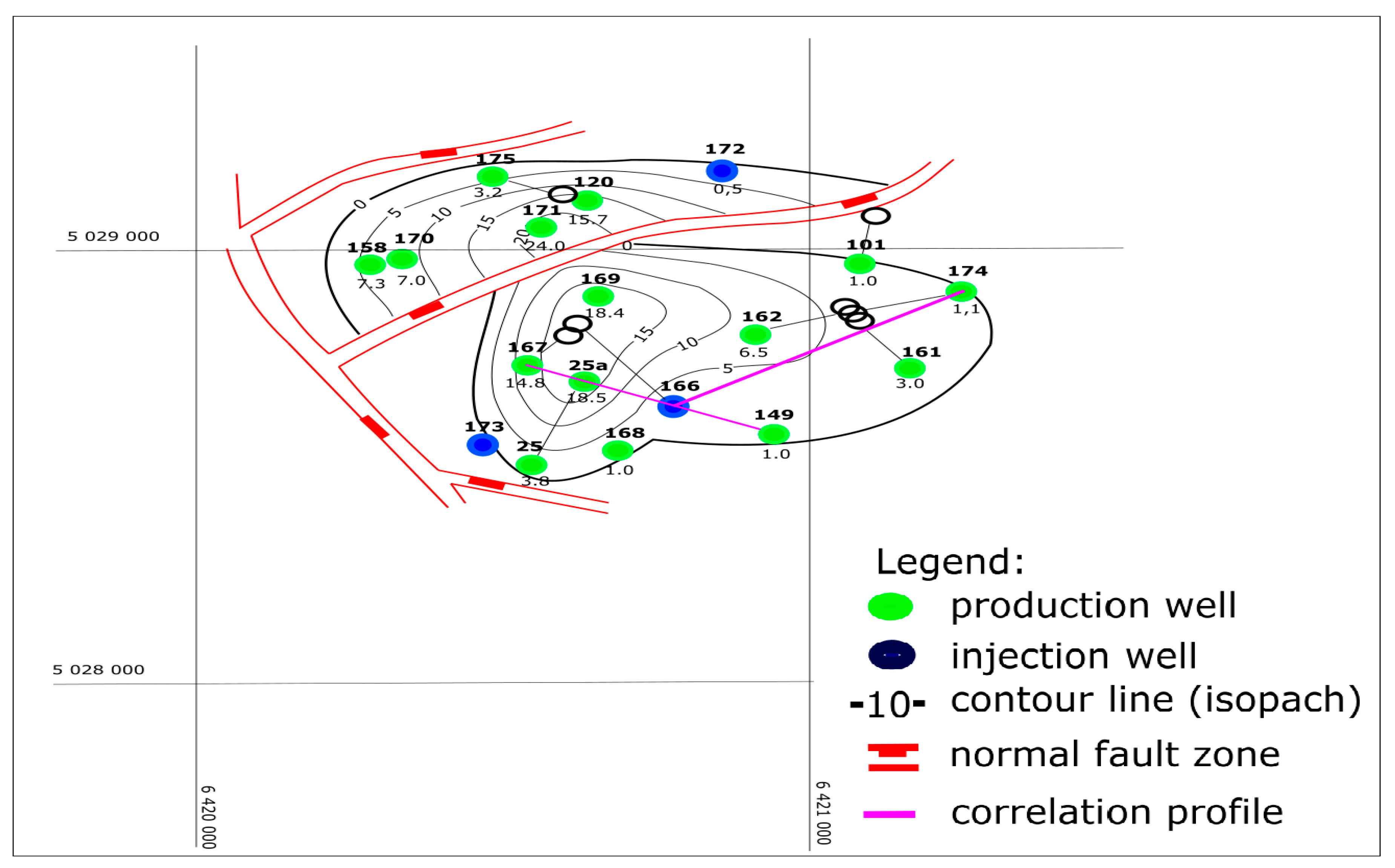
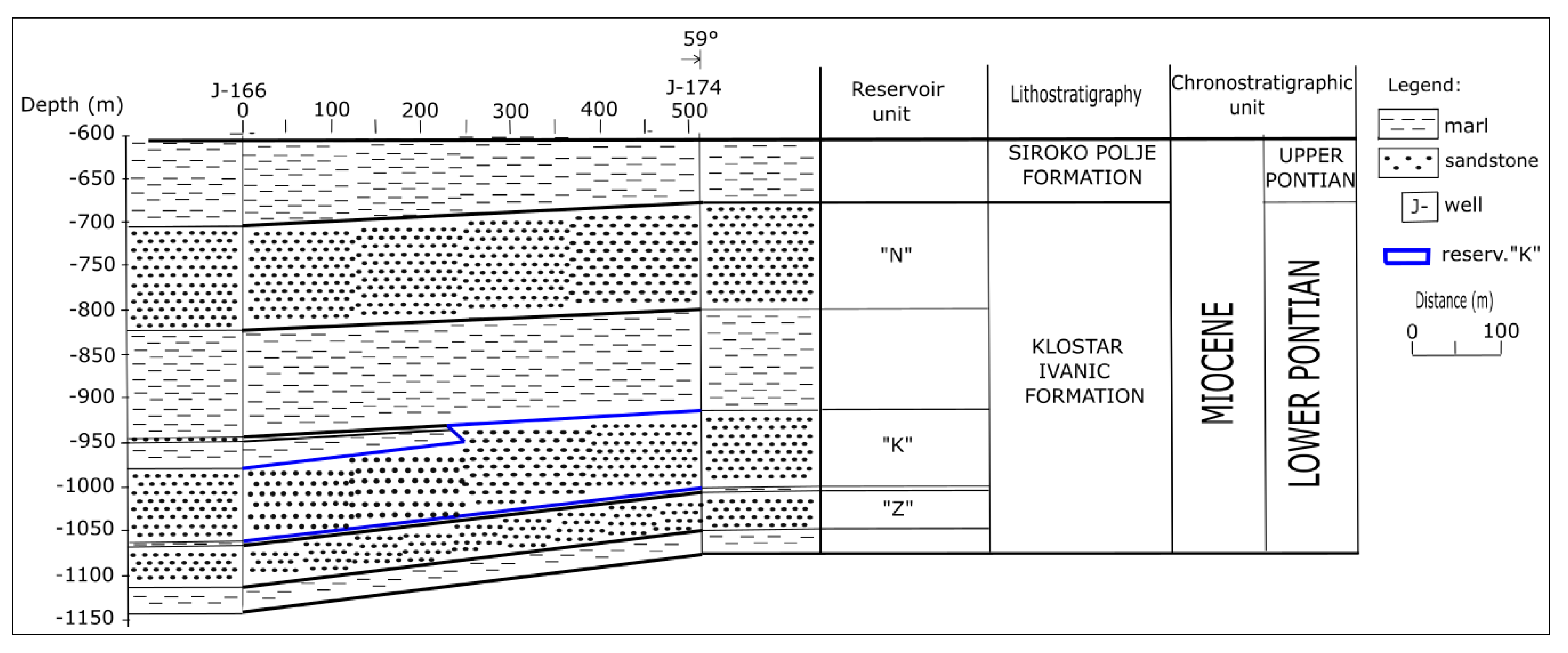
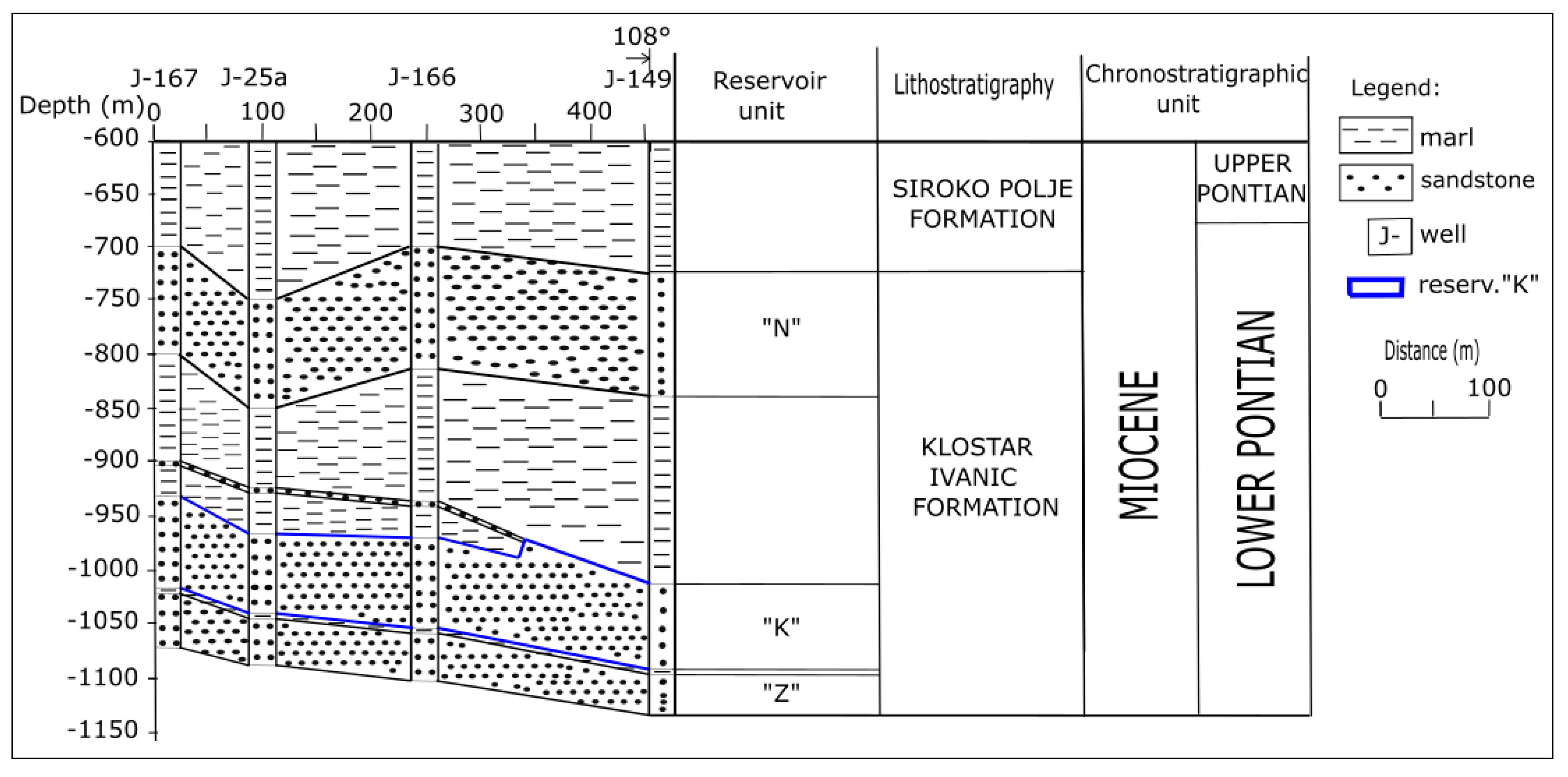
3.1.3. Structural Settings

The isopach map of reservoir “L” is given in Figure 9. The selected cross-sections are presented in Figure 10 and Figure 11. The thickness of reservoirs in the Kloštar Ivanić Formation (Figure 10) are mostly constant in the central part (reservoir “N” about 150 m, “B” 20 m, “K” and “JL” 80 m, and “L” 45 m). However, the analyzed reservoir “L” thinned from 70 m (L-161) to only 20 m (L-153). Similar is seen at the section SW–NE (Figure 11), where the thickness of the reservoir “L” from 20 m (L-63, L-57, L-27) gradually increases to 39 m (L-131alfa).

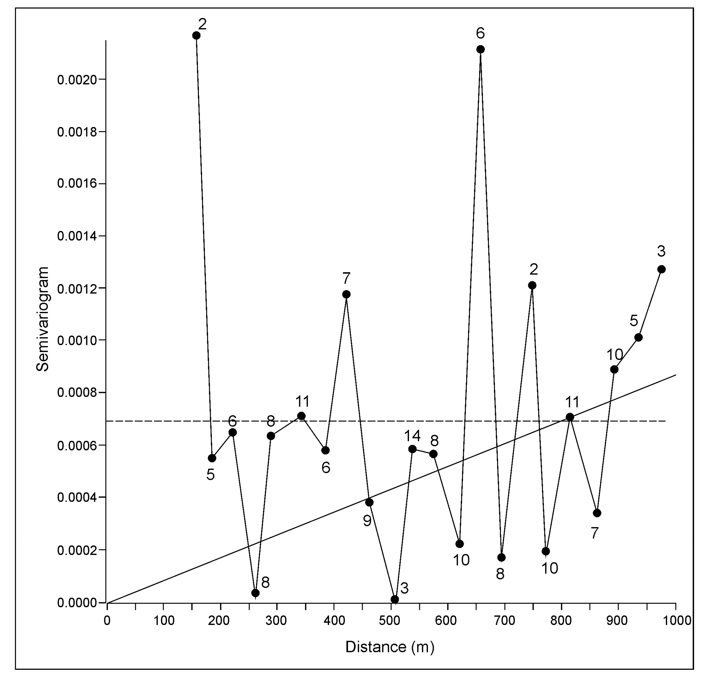
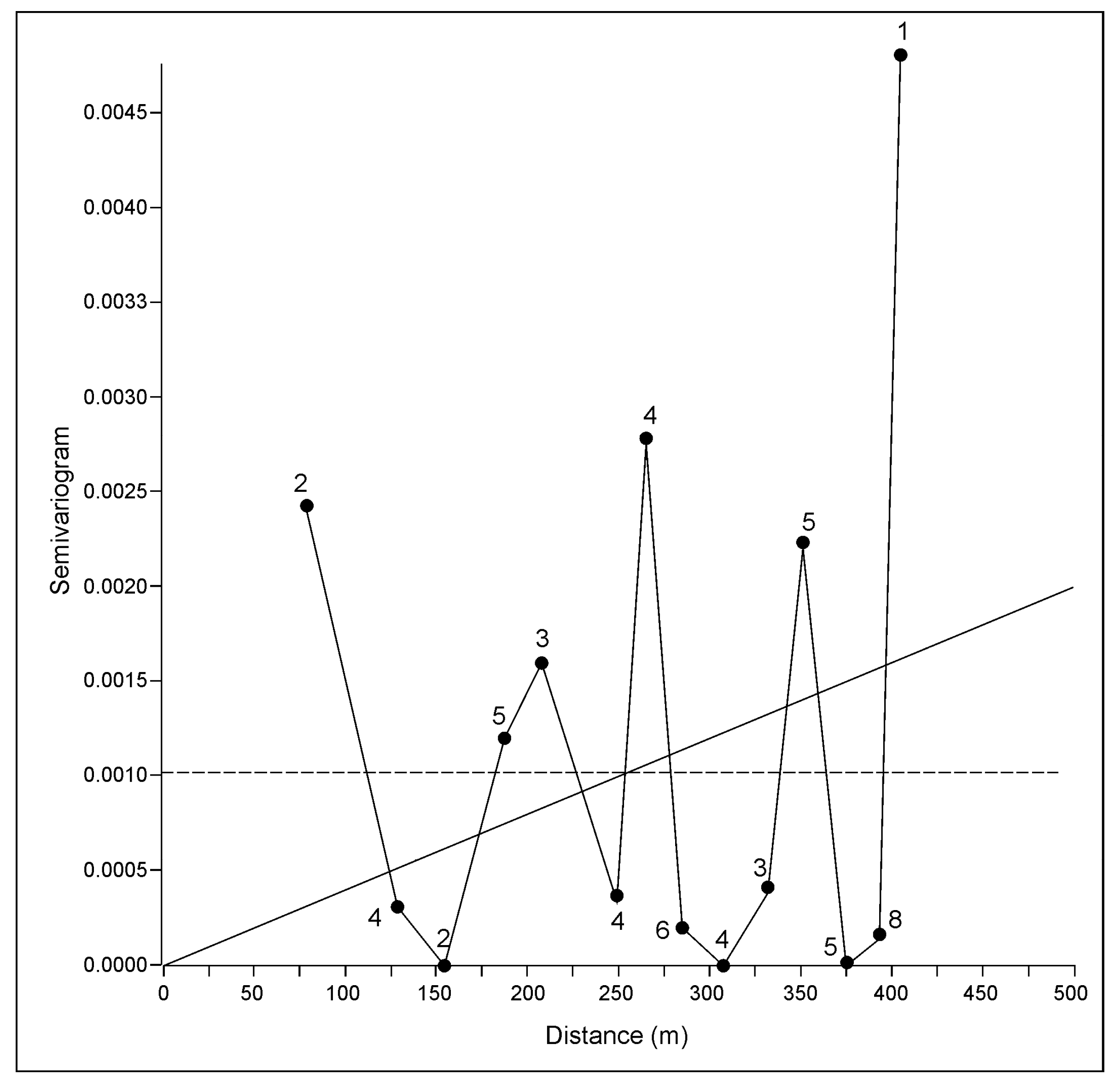
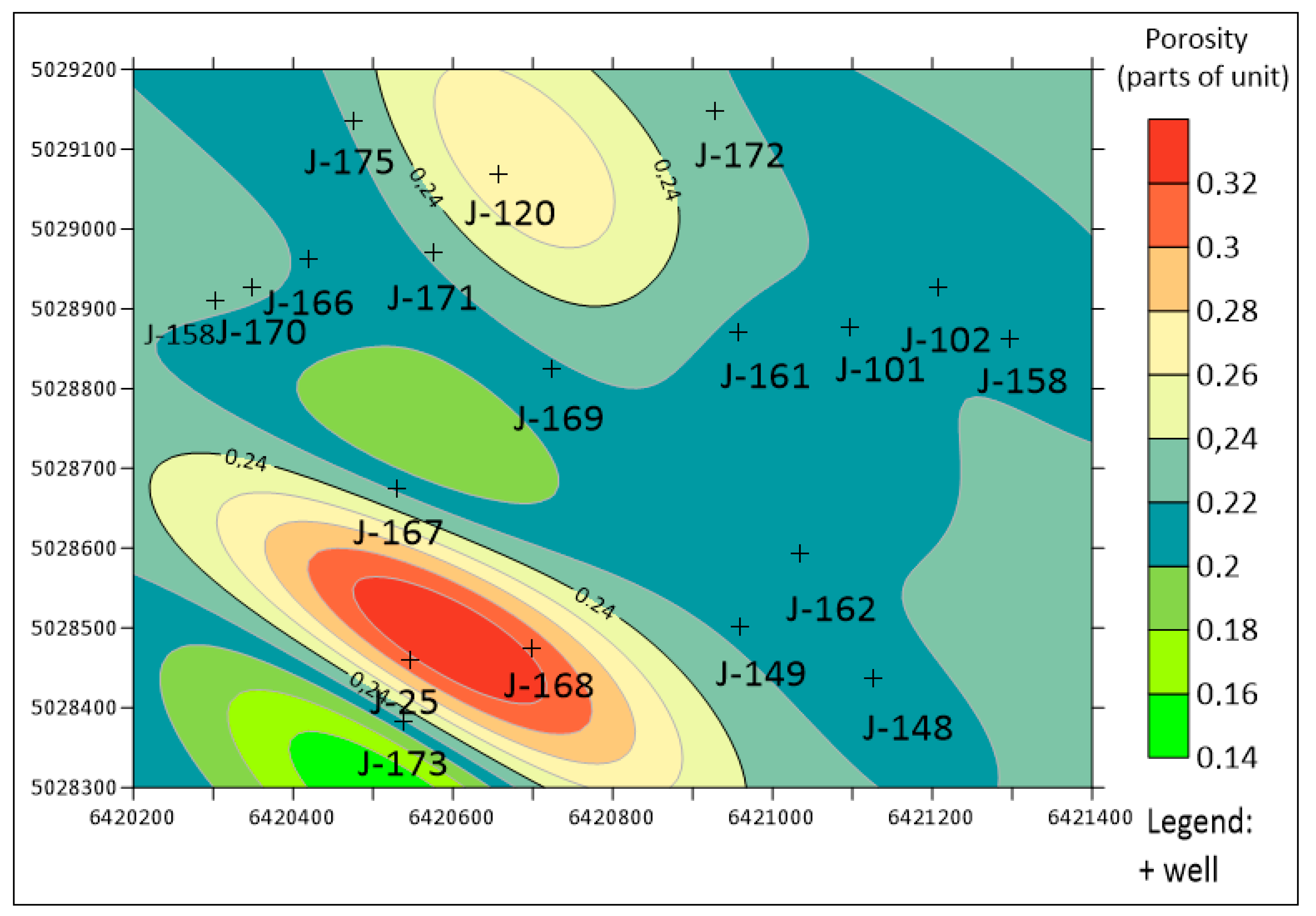
3.1.4. Variogram Analysis and Ordinary Kriging of Porosity

The porosity data was available in 25 wells (Figure 12). The previously interpolated porosity maps were too simplified, mostly including one average value for a single tectonic block. Moreover, kriging has been proven as the most appropriate method for interpolation of different variables in the Upper Miocene sandstone reservoirs of the CPBS (e.g., [2,8,10,18]). This is why, the for selected reservoir, the experimental semivariogram for available porosities had been calculated (Figure 13), and kriging was applied.

Unfortunately, the semivariogram is characterized by large oscillations and a low number of data pairs per class. Thus, the approximation was possible only with the simplest, linear, model. The ordinary kriging map is shown in Figure 14.

The cross-validation (where porosity is expressed as parts of units, not as percentages) for the kriged map is 0.000676. However, the variogram model is obviously characterized with large uncertainties (estimation of nugget, number of data pairs). This is why it has been decided to apply the jack-knifing statistical method with the purpose of artificially increasing the number of data points. Jack-knifing had been a previously applied or described in the CPBS [3,39]. Basically, this method has a similar algorithm as cross-validation, where data or groups of data have been “deleted” and the estimation is done from the rest. Such a re-sampling method is characterized by standard error (e.g., [40,41,42]) and can be used as one of the improvements in the basic kriging techniques or data intended to interpolate using kriging (e.g., digital terrain model (DTM) data, as in [43]).

In this study, jackknifing had been applied for each variogram class (step), which was calculated several times. The final value was the approximation of each calculation set for the same class (lag). The lag (of class of data) has been determined experimentally, i.e., in several iterations. The selected lag tolerance was half the lag value, so there was no overlapping of data in two classes. The value of the lag did not change significantly in the (a) shape of oscillation or (b) number of data pairs per class, which indicated that the number of original data points was too small for an advanced and more reliable spatial (variogram) modelling.

Consequently, the number of data pairs included in the calculation of class was much larger. The “jack-knifed” semivariogram for the same reservoir porosity is given in Figure 15. Oscillations are largely decreased in several points, and the experimental semivariogram is approximated with the exponential theoretical model, significantly decreasing the range.

Using the new semivariogram, the new porosity map was interpolated (Figure 16). Due to a much smaller range, the new porosity map is characterized with numerous “bull-eye” shapes.

3.2. The Field “B”, Reservoir “K”, Hydrodynamic Unit “K1”

3.2.1. Reservoir Type

According to [37], the reservoirs in the field “B” are of bedding type, capped by isolators, and margined with lithological and/or tectonic screens. In that brachianticline, with a northwest–southeast strike, sandstone reservoirs are enriched by mica minerals and quartz and occasionally interbedded with marls and (shallower) sandy marls. The “K” reservoir is divided into several tectonic blocks, where each is a mostly separated hydrodynamic (HD) unit. This is the largest such unit analyzed here (the HD “K1”).

3.2.2. Granulometry, Porosity, Saturation and Permeability of Sandstones

The granulometry is shown in

Table 2. Granulometry of reservoir “K” (M_d—mean grain diameter, S_o—coefficient of sorting, S_k—coefficient of asymmetry) (from archive of INA Plc.).

Well	Md	So	Sk	Sand (%)	Coarse Silt (%)	Clay (%)	CaCO3 with Gran. (%)	CaCO3 (%)
25	0.071	1.560	1.239	56	44	0	30.1	14
31	0.101	1.430	0.980	76	24	0	28.4	4
33	0.099	1.660	1.100	75	25	0	35.4	1
45	0.094	1.496	1.445	85	15	0	28.8	1
55	0.094	1.461	1.172	77	23	0	27.6	41
57	0.037	1.564	1.251	28	72	0	20.4	2
59	0.095	1.460	1.150	79	21	0	27.0	15
68	0.098	1.530	1.300	53	21	0	28.7	1
120	0.065	1.167	1.044	72	47	0	31.2	18

. The porosity was calculated for cores in 3 wells (27.2–31.5%) and logs in 36 wells (18.2–22.3% in gas saturated and 18.3–24.9% in oil saturated part). The saturation was determined using a laboratory in 32 wells and from logs in 36 wells. S_g is 69.3–79.5% and S_o 52.8–71.6%. The permeability (in 3 wells) is 29.6–121.2 × 10⁻³ µm².

3.2.3. Structural Settings

The HD “K1” unit is the largest tectonic block and HD in the reservoir “K”. The part where the reservoir pressure is supported by water injection is given in Figure 17.

This reservoir has been crossed with two sections (Figure 17). The first has strike approximately NW–SE (Figure 18), and the second NE–SW (Figure 19). The section in Figure 18 shows that the reservoirs have similar thickness in both wells (“N” about 120 m, “K” 100 m, “Z” 40 m). Some marls pinch out, which could define separated hydrodynamic units. The next section (Figure 19) clearly shows partial structural inversion in the Kloštar Ivanić Formation, i.e., transition from monocline (deeper) to fold (shallower).

3.2.4. Variogram Analysis and Ordinary Kriging of Porosity

Porosity data were available in 19 wells (Figure 20). The porosity data were analyzed using a semivariogram, and the experimental one is shown in Figure 21.

Due to large uncertainties and a small number of data pairs, the semivariogram is approximated with a simple linear model. Such a model did not allow the estimation of nugget and certain range. It was applied in ordinary kriging and resulting map is shown in Figure 22. The cross-validation is 0.0013197.

Again, the new semivariogram was calculated with “re-sampled”, i.e., jack-knifed, dataset. The “one-leave-out” technique was used here, i.e., the jack-knife estimation was done for each sub-dataset where the i-th data was omitted (i = 1, n; n is total number of data points). Practically, this means that each variogram value per lag was calculated n times, and averaged. The direct consequence is that the number of data pairs per lag (class) was drastically increased, e.g., for the distance 80 m it was increased from 2 to 32 data pairs, and secondly, the lag distance could be decreased.

The new experimental model is given in Figure 23. This could be approximated with the Gaussian theoretical model and the resulting kriging map is shown in Figure 24. The semivariogram sill is lower and range larger (based on goodness of fit) than in the previous variogram model based on the original dataset (19 points). The new kriged porosity map is shown in Figure 24 and the accompanying cross-validation value is 0.0009704.

4. Discussion and Conclusions

The presented analysis is the first of such a kind in the Sava Depression (Northern Croatia). It represents the continuation of previous geostatistical analyses conducted in that depression and the entire CPBS. The permanent problem of small datasets is emphasized as crucial for the subsurface mapping of different geological variables. In numerous analyzes, new hard data can hardly be obtained, mostly due to the costs of drilling (logging or seismic). Consequently, any statistical method that could increase the reliability of existing datasets and their analytical results is more than welcome. Jack-knifing is one such method. Previously, it was successfully applied in the (adjacent) Drava Depression, and here, for the first time, in the Sava Depression. The method could be highly appropriate for datasets of 15–30 points, where the basic, descriptive statistics are more or less representative (variance and mean), and the Gaussian distribution can be assumed.

In both analyzed reservoirs, the original semivariogram results were highly uncertain, with large oscillations, a small number of data pairs per class and unknown nugget. Consequently, the linear model was the only acceptable theoretical model to use. This was why a much larger number of re-sampled data points was calculated using jack-knifing. As a result, the new semivariograms could be approximated more reliably and with mathematically advanced theoretical models (exponential and Gaussian).

The hypothesis that new kriged maps interpolated from “jack-knifed” semivariograms are more reliable was eventually tested (a) visually (maps without the “bull-eye” or “butterfly” effects are better) and (b) numerically, using cross-validation. The, so called “bull-eyes” or “butterflies” have the same origin, and both can indicate contradiction between the data and the spatial continuity model. Such contradiction is the result of the “computing algorithm”, which allows us to have two contour lines of the same value in the same point. However, the probability for such an event is almost infinitesimally low. This is why two such effects (both are similar, but the bull-eye is mostly circular and the butterfly ellipsoidal) indicate errors in the applied algorithm, the majority resulting from small spatial continuity (such as variogram range).

The results are given in

Table 3. Comparison of cross-validation values for ordinary kriging (OK) maps based on original and jack-knifed semivariograms (IDW: inverse distance weighting).

Field/Reservoir	OK (Original Semivariogram)	OK (Jack-Knifed Semivariogram)	Recommendation
“A”/“L”	0.000676 (linear)	0.000420 (exponential)	OK with original semivariogram or IDW. The effect of “bull-eyes” eliminated the jack-knifed approach.
“B”/“K1”	0.001320 (linear)	0.000970 (Gaussian)	OK with jack-knifed semivariogram

and point out that:

(1)

When experimental semivariograms are described with large uncertainties it is recommended that the variogram is repeated using jack-knifed resampling, and followed by the kriging interpolation.

(2)

Any map from the set of “old” or “new” data/semivariograms firstly needs to be visually checked. If effects such as “bulls-eye” or “butterfly” shapes are numerous, the map needs to be eliminated.

(3)

If both kriged maps (based on original and jack-knifed datasets) are visually (geologically) acceptable, the selection can be done based on cross-validation values.

(4)

For small data sets (less than 15 data points) it is also recommended to interpolate with inverse distance weighting and compare both with ordinary kriging (OK) and inverse distance weighting (IDW) results.

The presented test of the jack-knifing was conducted for the sandstone reservoir porosity. The selected fields (“A”, “B”) and reservoirs (“L”, “K1”) represent typical Upper Miocene sandstones in the Sava Depression, with a portion of sandy detritus 50–72% and porosity 14.5–23.9% (“A”), i.e., 21.7–31.5% (“B”). This is why these conclusions could be applied to any other such reservoirs of the Sava Depression and the Kloštar Ivanić Formation.

References

1. Malvić, T.; Velić, J.; Peh, Z. Qualitative-Quantitative Analyses of the Influence of Depth and Lithological Composition on Lower Pontian Sandstone Porosity in the Central Part of Bjelovar Sag (Croatia). Geol. Croat. 2015, 58, 73–85. [Google Scholar]
2. Malvić, T. Production of a porosity Map by Kriging in Sandstone Reservoirs, Case study from the Sava Depression. Kartografija i Geoinf. 2008, 9, 12–19. [Google Scholar]
3. Malvić, T.; Bastaić, B. Reducing variogram uncertainties using the “jack-knifing” method, a case study of the Stari Gradac—Barcs-Nyugat field. Bull. Hung. Geol. Soc. 2008, 138, 165–174. [Google Scholar]
4. Malvić, T. Stochastical approach in deterministic calculation of geological risk—Theory and example. Nafta 2009, 60, 658–662. [Google Scholar]
5. Malvić, T.; Balić, D. Linearnost i Lagrangeov linearni multiplikator u jednadžbama običnoga kriginga (Linearity and Lagrange Linear Multiplicator in the Equations of Ordinary Kriging). Nafta 2009, 60, 31–43. [Google Scholar]
6. Novak Zelenika, K.; Malvić, T. Procjena sekvencijskim Gaussovim simulacijama ležišnih varijabli pješčenjačkog donjopontskoga ležišta nafte, polje Kloštar, Savska depresija, Hrvatska (Estimations by sequential Gaussian simulations of reservoir variables in Early Pontian oil reservoir, Kloštar Field, Sava Depression, Croatia). In Proceedings of the 4. Croatian Geological Congress with International Participation, Šibenik, Croatia, 14–15 October 2010; Horvat, M., Ed.; Croatian Geological Institute: Sachsova, Zagreb, 2010; pp. 263–264. [Google Scholar]
7. Malvić, T. Kriging, cokriging or stohastical simulations, and the choice between deterministic or sequential approaches. Geol. Croat. 2008, 61, 37–47. [Google Scholar]
8. Novak Zelenika, K.; Malvić, T.; Geiger, J. Mapping of the Late Miocene sandstone facies using indicator kriging. Nafta 2010, 61, 225–233. [Google Scholar]
9. Novak Zelenika, K.; Malvić, T. Stochastic simulations of dependent geological variables in sandstone reservoirs of Neogene age: A case study of Kloštar Field, Sava Depression. Geol. Croat. 2011, 64, 173–183. [Google Scholar] [CrossRef]
10. Novak Zelenika, K. Deterministički i stohastički geološki modeli gornjomiocenskih pješčenjačkih ležišta u naftno-plinskom polju Kloštar (Deterministic and Stochastic Geological Models of Upeer Miocene Sandstone Reservoirs at the Kloštar Oil and Gas Field). Ph.D. Thesis, Faculty of Mining, Geology and Petroleum, University of Zagreb, Zagreb, Croatia, 2012. [Google Scholar]
11. Malvić, T. History of geostatistical analyses performed in the Croatian part of the Pannonian Basin System. Nafta 2012, 63, 223–235. [Google Scholar]
12. Husanović, E.; Malvić, T. Review of deterministic geostatistical mapping methods in Croatian hydrocarbon reservoirs and advantages of such approach. Nafta 2014, 65, 57–63. [Google Scholar]
13. Novak Zelenika, K.; Malvić, T. Utvrđivanje sekvencijskim indikatorskim metodama slabopropusnih litofacijesa kao vrste nekonvencionalnih ležišta ugljikovodika na primjeru polja Kloštar (Determination of Low Permeable Lithofacies, as Type of Unconventional Hydrocarbon Reservoirs, Using Sequential Indicator Methods, Case Study from the Kloštar Field). Rudarsko-geološko-naftni zbornik (Min.-Geol.-Pet. Eng. Bull.) 2014, 28, 23–38. [Google Scholar]
14. Malvić, T.; Velić, J. Stochastically improved methodology for probability of success (POS) calculation in hydrocarbon systems. RMZ-Mater. Geoenviron. 2015, 62, 149–155. [Google Scholar]
15. Novak Mavar, K. Modeliranje površinskoga transporta i geološki aspekti skladištenja ugljikova dioksida u neogenska pješčenjačka ležišta Sjeverne Hrvatske na primjeru polja Ivanić (Surface Transportation Modelling and Geological Aspects of Carbon-Dioxide Storage into Northern Croatian Neogene Sandstone Reservoirs, Case Study Ivanić Field). Ph.D. Thesis, Faculty of Mining, Geology and Petroleum, University of Zagreb, Zagreb, Croatia, 2015. [Google Scholar]
16. Špelić, M.; Malvić, T.; Saraf, V.; Zalović, M. Remapping of depth of e-log markers between Neogene basement and Lower/Upper Pannonian border in the Bjelovar Subdepression. J. Maps 2016, 12, 45–52. [Google Scholar] [CrossRef]
17. Mesić Kiš, I. Odabir interpolacijskog algoritma primjerenog za kartiranje naftno-plinskog polja Šandrovac (Selection of interpolation algorithm appropriate for mapping of oil and gas Šandrovac Field). In Proceedings of the Symposium PhD Students of Science, Zagreb, Croatia, 26 February 2016; Primožić, I., Hranilović, D., Eds.; Faculty of Science, University of Zagreb: Zagreb, Croatia, 2016; p. 64. [Google Scholar]
18. Mesić Kiš, I. Kartiranje i reinterpretacija geološke povijesti Bjelovarske subdepresije univerzalnim krigiranjem te novi opći metodološki algoritmi za kartiranje sličnih prostora (Mapping and Reinterpretation of the Geological Evolution of the Bjelovar Subdepression by Universal Kriging and New General Methodological Algorithms for Mapping in Similar Areas). Ph.D. Thesis, Faculty of Science, University of Zagreb, Zagreb, Croatia, 2017. [Google Scholar]
19. Malvić, T. Stochastics—Advantages and uncertainties for subsurface geological mapping and volumetric or probability calculations. Mater. Geoenviron. 2018, 65, 9–19. [Google Scholar] [CrossRef]
20. Ivšinović, J. Deep mapping of hydrocarbon reservoirs in the case of a small number of data on the example of the Lower Pontian reservoirs of the western part of Sava Depression. In Proceedings of the 2nd Croatian Congress on Geomathematics and Geological Terminology, Zagreb, Croatia, 6 October 2018; Malvić, T., Velić, J., Rajić, R., Eds.; Faculty of Mining, Geology and Petroleum, University of Zagreb: Zagreb, Croatia, 2018; pp. 59–65. [Google Scholar]
21. Gringarten, E.; Deutsch, C.V. Methodology for Variogram Interpretation and Modeling for Improved Reservoir Characterization. In Proceedings of the SPE Annual Technical Conference and Exhibition, Houston, TX, USA, 3–6 October 1999. SPE-56654-MS. [Google Scholar] [CrossRef]
22. Gringarten, E.; Deutsch, C.V. Teacher’s Aide Variogram Interpretation and Modeling. Math. Geol. 2001, 33, 507–534. [Google Scholar] [CrossRef]
23. Journel, A.G.; Alabert, F.G. New Method for Reservoir Mapping. J. Pet. Technol. 1990, 40, 7. [Google Scholar] [CrossRef]
24. Wenlong, X.; Tran, T.T.; Srivastava, R.M.; Journel, A.G. Integrating seismic Data in Reservoir Modeling: The Collocated Cokriging Alternative. Proc. SPE 1992, 24742, 833–842. [Google Scholar]
25. Al-Mudhafar, W.J. Integrating Core Porosity and Well Logging Interpretations for Multivariate Permeability Modeling through Ordinary Kriging and Co-Kriging Algorithms. In Proceedings of the Offshore Technology Conference, Houston, TX, USA, 30 April–3 May 2018. OTC-28764-MS. [Google Scholar] [CrossRef]
26. Al-Mudhafar, W.J. Bayesian kriging for reproducing reservoir heterogeneity in a tidal depositional environment of a sandstone formation. J. Appl. Geophys. 2019, 160, 84–102. [Google Scholar] [CrossRef]
27. Ortiz, J.C.; Deutsch, C.V. Calculation of Uncertainty in the Variogram. Math. Geol. 2002, 34, 169–183. [Google Scholar] [CrossRef]
28. Olea, R.A.; Pardo-Iguzquiza, E. Generalized Bootstrap Method for Assessment of Uncertainty in Semivariogram Inference. Math. Geosci. 2011, 43, 203–228. [Google Scholar] [CrossRef]
29. Journel, A.G.; Huijbregts, C.J. Mining Geostatistics; Academic Press: London, UK, 1978; 600p. [Google Scholar]
30. Hohn, M.E. Geostatistics and Petroleum Geology; Van Nostrand Reinhold: New York, NY, USA, 1988; 400p. [Google Scholar]
31. Liebhold, A.M.; Rossi, R.E.; Kemp, W.P. Geostatistics and Geographic Information System in Applied Insect Ecology. Ann. Rev. Entomol. 1993, 38, 303–327. [Google Scholar] [CrossRef]
32. Velić, J.; Malvić, T.; Cvetković, M. Geologija i istraživanje ležišta ugljikovodika (Geology and Exploration of Hydrocarbon Reservoirs); Faculty of Mining, Geology and Petroleum Zagreb, University of Zagreb: Zagreb, Croatia, 2015; p. 144. ISBN 978-953-6923-28-1. [Google Scholar]
33. Malvić, T. Review of Miocene shallow marine and lacustrine depositional environments in Northern Croatia. Geol. Q. 2012, 56, 493–504. [Google Scholar] [CrossRef] [Green Version]
34. Royden, L.H. Late Cenozoic tectonics of the Pannonian Basin System. AAPG 1988, 45, 27–48. [Google Scholar]
35. Pavelić, D.; Kovačić, M. Sedimentology and stratigraphy of the Neogene rift-type North Croatian Basin (Pannonian Basin System, Croatia): A review. Mar. Pet. Geol. 2018, 91, 455–469. [Google Scholar] [CrossRef]
36. Malvić, T.; Velić, J. Neogene Tectonics in Croatian Part of the Pannonian Basin and Reflectance in Hydrocarbon Accumulations. In New Frontiers in Tectonic Research: At the Midst of Plate Convergence; Schattner, U., Ed.; InTech: Rijeka, Croatia, 2011; pp. 215–238. ISBN 978-953-307-594-5. [Google Scholar]
37. Vrbanac, B.; Velić, J.; Malvić, T. Sedimentation of deep-water turbidites in main and marginal basins in the SW part of the Pannonian Basin. Geol. Carpath. 2010, 61, 55–69. [Google Scholar] [CrossRef]
38. Brod, I.O. Geological Terminology in Classification of Oil and Gas Accumulation. AAPG Bull. 1945, 29, 1738–1755. [Google Scholar]
39. Malvić, T.; Vrbanac, B. Geostatistički pojmovnik (Geostatistical Glossary). Hrvatski Matematički Elektronički Časopis 2013, 23, 7–56. [Google Scholar]
40. Wu, C.F.J. Jackknife, Bootstrap and Other Resampling Methods in Regression Analysis. Ann. Stat. 1986, 14, 1261–1295. [Google Scholar] [CrossRef]
41. Shao, J. Jackknifing in generalized linear models. Ann. Stat. 1992, 44, 673–686. [Google Scholar] [CrossRef]
42. McIntosh, A.I. The Jackknife Estimation Method, Cornell University Library. 2016. Available online: https://arxiv.org/abs/1606.00497 (accessed on 20 November 2018).
43. Wojciech, M. Kriging Method Optimization for the Process of DTM Creation Based on Huge Data Sets Obtained from MBESs. Geosciences 2018, 8, 433. [Google Scholar] [CrossRef]
Figure 1. Regional geological units of the 2nd order (depressions in the CPBS) and location of the fields “A” and “B” (boxed) in the Sava Depression (from [32]).
Geosciences 09 00036 g001
Figure 2. Satellite maps of the fields “A” and “B” (taken from Google). The figure represents the area boxed in Figure 1, and locations of analyzed fields.
Geosciences 09 00036 g002
Figure 3. Regional geological units of the 1st order in the Pannonian Basin System (PBS) (modified from [33,34]). The Sava Depression is located at very southwestern margin (blue circle).
Geosciences 09 00036 g003
Figure 4. Timescale of the main tectonic and depositional events during Neogene and Quaternary in the CPBS [36]. Analyzed sandstone reservoirs belong to Early Pontian stage, i.e., to late 2nd transtensional phase.
Geosciences 09 00036 g004
Figure 5. Schematic view of regional lacustrine environments at the border of the Sava and Drava Depressions re-formatted from [36]. The huge amount of pelitic (marlstone) and turbiditic (sandstone, siltstone) clastics had been deposited [33,37].
Geosciences 09 00036 g005
Figure 6. Typical geological column for the fields “A” and “B”. The formal and informal lithostratigraphic units are listed.
Geosciences 09 00036 g006
Figure 7. The composite log-lithological column in the field “A” (from archive of INA Plc. and re-drawn).
Geosciences 09 00036 g007
Figure 8. The composite log-lithological column in the field “A” (from archive of INA Plc. and re-drawn).
Geosciences 09 00036 g008
Figure 9. Isopach map of part of the reservoir “L”, where reservoir pressure is supported with water injection (from archive of INA Plc. and re-drawn).
Geosciences 09 00036 g009
Figure 10. Cross-section through wells L-161—L-153—L-27.
Geosciences 09 00036 g010
Figure 11. Cross-section section through wells L-163—L-57—L-27—L-131alfa.
Geosciences 09 00036 g011
Figure 12. Porosity data available for reservoir “L” (from archive of INA Plc. and re-drawn).
Geosciences 09 00036 g012
Figure 13. Experimental semivariogram with approximation, reservoir “L”, porosity.
Geosciences 09 00036 g013
Figure 14. Porosity map for reservoir “L” interpolated by ordinary kriging.
Geosciences 09 00036 g014
Figure 15. Experimental semivariogram with approximation, reservoir “L”, porosity, after jack-knifing.
Geosciences 09 00036 g015
Figure 16. Porosity map for reservoir “L” interpolated by ordinary kriging with jack-knifed semivariogram.
Geosciences 09 00036 g016
Figure 17. Isopach map of the HD unit “K1”, where reservoir pressure is supported with water injection (from archive of INA Plc.).
Geosciences 09 00036 g017
Figure 18. Correlation section through wells J-166—J-174.
Geosciences 09 00036 g018
Figure 19. Correlation section through wells J-167—J-25alfa—J-166—J-149.
Geosciences 09 00036 g019
Figure 20. Porosity data available for HD “K1” (from archive of INA Plc.).
Geosciences 09 00036 g020
Figure 21. Experimental semivariogram with approximation, reservoir/HD “K1”, porosity.
Geosciences 09 00036 g021
Figure 22. Porosity map for reservoir/HD “K1” interpolated by the Ordinary Kriging.
Geosciences 09 00036 g022
Figure 23. Experimental semivariogram with approximation, reservoir/HD “K1”, porosity, after jack-knifing.
Geosciences 09 00036 g023
Figure 24. Porosity map for reservoir/HD “K1” interpolated by ordinary kriging with jack-knifed semivariogram.
Geosciences 09 00036 g024