An Improved Strength Reduction-Based Slope Stability Analysis


1
X-Elastica, LLC, Boulder, CO 80303, USA
2
School of Natural and Built Environment, University of South Australia, 5001 Adelaide, Australia
3
Department of Civil Environmental and Architectural Engineering, University of Colorado, Boulder, CO 80309, USA
*
Author to whom correspondence should be addressed.
Geosciences 2019, 9(1), 55; https://doi.org/10.3390/geosciences9010055
Submission received: 15 November 2018
/
Revised: 11 January 2019
/
Accepted: 16 January 2019
/
Published: 21 January 2019
Abstract
:Slope uncertainty predominantly originates from the imperfect analysis model and the inaccuracy and imprecision of the observations. The strength reduction method (SRM) is widely used to attain the safety factor (SF) of the slopes, which is similar to interpretation of the limit state (LS). In this paper, the spectral element method (SEM), using an elasto-plastic Mohr–Coulomb failure criterion, is employed to project the plausible LS of the soil slopes. An iterative SRM search method is proposed to evaluate the SF of the slopes regardless of the LS interpretation. The proposed SRM paradigm encompasses the design trigger to trace the uncertain parameters in decision-making. This method is applied to three numerical examples: (1) a homogeneous dry slope, (2) a dry slope with a weak layer, and (3) a partially-wet slope with a weak layer. It is shown that for the case study examples, the proposed SRM reasonably converges to the required precision. Results further are compared and contrasted with some of the conventional and standard techniques in slope stability. This hybrid procedure paves the road for fast and safe stability analysis of man-made and natural slopes.
1. Introduction
Slope stability analysis is one of the most important research fields in geoscience. Slope stability models are associated with many uncertainty sources, such as material properties [1], simulation methods [2], failure path, and applied loads. Numerous researchers have proposed a wide spectrum of analysis techniques (ranging from simple/approximate to detailed/complex numerical models) to evaluate the slope stability. From the perspective of the soil stability analysis, there are two widely-used analysis methods: (1) the limit equilibrium method (LEM) and (2) the strength reduction method (SRM).
Some of the fundamental research related to the LEM can be found in Spencer [3], Sarma [4]. The limitations of the LEM have been well discussed by Krahn [5]. The LEM is based on a predefined hypothetical failure surface with a rigid (i.e., unconformable) super-structure [6]. It is assumed that there are two forces acting on the rigid body, i.e., the driving force, which attempts to move the rigid body, and the resisting force which prevents this action. The slope is considered to be stable as long as the resisting forces are greater than or equal to the driving ones, and their ratio is called the safety factor (SF). Therefore, the LEM is deemed a deterministic approach for soil stability analysis [7].
On the other hand, the application of SRM has also gained popularity in slope stability assessment. It was employed by Dawson et al. [8], Griffiths and Lane [9], Matsui and San [10], and Ugai [11] for the calculation of the safety factor in soil slopes. In SRM, the shear strength of the soil is reduced to trigger the failure of the slope. The reduction factor imposed on the system at the failure threshold is designated as the safety factor. Although many strategies have been introduced for the definition of the trigger of the failure [12,13], the deterministic assumption and engineering judgment imply the model uncertainties.
Although many of the current slope stability applications are focused on the numerical discretization with the crude finite element method (FEM), several variations are also proposed, e.g., spectral element method (SEM), extended FEM (XFEM), boundary element method (BEM), smoothed FEM (SFEM), etc. Of particular interest is SEM to solve the boundary value problems. The SEM is, in fact, a high-order form of the FEM suitable for geotechnical engineering problems. Gharti et al. [14] introduced the SEM for the evaluation of 3D soil slope stability. Many other researchers have shown the application of SEM in different geomechanics and geotechnical engineering problems. Among them are: the effect of geometrics on 3D slope stability by Zhang et al. [15], the assessment of the vegetated and barren soil slopes by Tiwari et al. [16], the seismic slope stability of natural slopes by Tiwari et al. [17], the evaluation of long and steep slopes by Tiwari et al. [18], simulations of the elastic wave propagation in exploration by Zheng et al. [19], and 3D rock stability by Shen and Karakus [20].
In this study, the stability of the soil slope is evaluated based on the spectral element method. An approach rooted in the design criteria is proposed to find the safety factor under the strength reduction method. First, the fundamentals of the slope stability analysis, spectral element method and strength reduction method are discussed. Next, the proposed method is explained, and several case study problems are analyzed to show the advantages of this hybrid method.
2. Fundamental Theories
2.1. Spectral Element Method
SEM is constituted of three general parts: pre-, main, and post-processing. The pre-processing itself consists of geometry, material attributes, and boundary conditions. Nodes’ coordinates and elements’ connectivities are the most important parameters that need to be defined for a proper application. The unit weight, , Young’s modulus, E, internal friction angle, , dilation angle, , and cohesion, c, are classified as material properties. Moreover, the boundary conditions must be applied carefully in order to develop a reliable simulation.
SEM is a flexible technique, which can adapt a variety of the element types and the arbitrary order of integration points via Gaussian quadrature from FEM [14]. Figure 1 illustrates the fundamental difference between SEM and FEM. Both of them employ the same number of Lagrangian interpolation points in identical locations within the element, while the integration points are different. The readers should note that the provided mass matrices are used only in the dynamic analysis, and they are shown for the completeness of the comparison between SEM and FEM.
SEM utilizes Gauss–Legendre–Lobatto (GLL) points as a nodal quadrature for which interpolation nodes coincide with the integration points. In particular, additional integration points in FEM, which are called Gauss–Legendre (GL) points, are generated at different positions compared to the interpolation points. This innovative change in the configuration of the SEM improves its capabilities in two ways. First, removing the interpolation to calculate the nodal quantities from quadrature points makes the problem computationally simple. Second, interpolating functions become orthogonal on quadrature points, resulting in a diagonal mass matrix (used only in the dynamic analysis). Both changes increase the accuracy and decrease the computational effort. From the constitutive relation point of view, the elasto-plastic Mohr–Coulomb failure criterion is used to simulate the material behavior.
The unstructured hexahedron mesh technique is used to prepare the desired geometry for subsequent simulation. Then, the GLL nodes are introduced in each element. The nodes, interpolation points, and GLL points of an element are shown in Figure 2. The first step in mesh generation based on a hexahedral element is to divide the full geometrical model into several elements with common surface and corner nodes; see Figure 2a. Next, the interpolation and GLL points are mapped by SEM for each element; see Figure 2b,c. Finally, the boundary conditions along with external loads are applied.
2.2. Strength Reduction Method
Slope stability requires a series of nonlinear elasto-plastic simulations based on Mohr–Coulomb criteria. In the strength reduction method, the actual strength parameters are reduced by a certain reduction factor as [21]:
where SRF is a strength reduction factor.
To obtain an accurate safety factor, it is important to trace the SRF gradually until the reduced strength parameters, and , yield the predefined limit state (LS). This traditional approach makes the problem iterative and subsequently increases the analysis time and effort. However, in the proposed method, an intelligent method is used to update the new SRF based on the old values. The SRF corresponding to an LS is designated as SF for the slope (i.e., SF = SRF). Therefore, a legitimate interpretation of the LS is important. There are various LS criteria to identify the slope failure such as experimental tests [22], limiting the shear stress on the potential failure surface [23], divergence of the computation problem [8], calculation of the total equivalent plastic strain zone [24], running-through of the yielding zone, or a prescribed generalized shear strain developed from the toe through the crest of the slope [25], a rapid increase in displacement [9], and the formulation of an initial value problem to trace the critical slide line [26].
The impacts of the material properties on the overall slope stability are also studied. Zheng et al. [27] and Duan et al. [26] investigated the effects of Young’s modulus and Poisson’s ratio on the soil stability analysis. Dawson et al. [8] claimed that the value of elasticity parameters (i.e., E and ) had little impact on the SF. Therefore, the effects of elasticity parameters will not be discussed in this paper.
3. Methodology
The strategy to implement the SEM on the soil slopes is illustrated in Figure 3. This procedure can be categorized into four steps. First, the geometrical model and the material properties are defined as input parameters, which can be obtained by surveying techniques and the in situ tests/measurements, respectively. Next, the computational model is built to obtain a realistic response in which the SEM and the Mohr–Coulomb relation are employed. Different outputs can be extracted; however, the maximum displacement is the most palpable metric. Finally, the SRM is iteratively repeated to find the target SF.
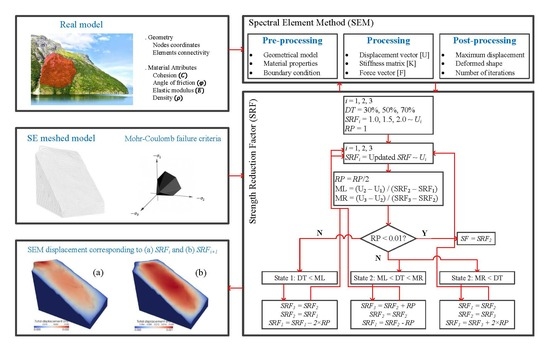
The proposed improved strength reduction method is presented in Figure 4. This flowchart shows that the main matrices in the SEM processing are displacement, , stiffness, , and the force vector, , which are developed in the pre-processing stage. Obviously, the processing stage is the most computationally demanding part, which is associated with the number of plastic nodes. The outputs are nodal displacement, deformed shapes, and the number of iterations.
It is noteworthy that the open-source software SPECFEM3D-GEOTECH was used in the present study, which can be found via Computational Infrastructure for Geodynamics (www.geodynamics.org). The software is parallelized on the basis of domain decomposition [14]. It can handle the material heterogeneity and complex models with significant topography. Both simple and variable free surface profiles may be used on the basis of a simple hydrostatic relation. To be used in the context of this paper, the above-mentioned software is coupled with [28] to perform the iterative simulations and automatically post-process the results.
As previously stated, the maximum displacement is used to evaluate SF based on the SRF. The proposed method is an automatic search technique, which is started with three SRFs, i.e., , , . Then, the maximum displacements, , corresponding to , are calculated. Figure 5a shows the variation of the maximum displacement to initialize the search parameters. The required precision (RP) is defined in order to automatize the process of SF determination. In other words, the iterative process will be repeated until the pre-defined RP is satisfied (it is set to 0.01 in this study). The SF corresponds to a rapid increase in the displacement response. The gradient of the displacement vs. SRF is considered as a design trigger (DT) to identify the LS. The DT is used to alleviate the aleatory selection of SF. Theoretically, the DT ranges from zero to infinity. However, in this study, three values are adopted, i.e., 30%, 50%, and 70%. The left and right gradients (denoted as MLand MR) are computed by Equation (3) to satisfy the DT constraint; see Figure 5b.
4. Case Study Models
Several examples have been simulated to evaluate and validate the slope stability analysis problems [14,29,30]. In this study, three slope stability problems are discussed: (1) homogeneous dry slope, (2) dry slope with a weak layer, and (3) partially-wet slope with a weak layer. All three case studies are symmetric in the XZ-plane [14]. Boundary conditions (BCs) are applied for half of the model in SEM; see Figure 6a. All the side faces are constrained in the perpendicular direction. The symmetry plane (back face) is free to move in the X and Z directions. The front face is further constrained in the vertical direction (due to a hypothetical valley). Since the bottom face is connected to the Earth, it is fully constrained.
5. Results and Discussion
5.1. Case 1
The dimensions and geometry of the first case study are illustrated in Figure 7a, which consist of 1670 elements and 2200 nodes. This model represents the dry region with material properties of = 18.8 kN/m, = 20, 29 kN/m, = 0, E = kN/m, and 0.3.
5.2. Cases 2 and 3
The dimensions and geometry of Case 2 and Case 3 are shown in Figure 7b, which consist of two different material types with 1890 elements and 2453 nodes. The highlighted weak layer is made of material properties with = 18.8 kN/m, = 0, 10 kN/m. The slope material properties are identical to Case 1.
5.3. Safety Factor Determination
The proposed algorithm in Section 3 was applied to the three case studies. In each case, three different DT margins were adopted, which were subsequently used to update the ML and MR values. The iteration process was continued until the RP reached 0.01.
In general, for the smaller SRF values, a simulation requires less iterations to fulfill the process (the system still behaves in the linear range). Increasing the SRF increases the number of plastic nodes. For example, in Case 1, with DT = 30%, the SEM required only 120 iterations for the system with SRF of 2.16 (elastic material), while it required more than 350 iterations for the system with SRF of 2.18 (which underwent plastic deformations). In Case 2 (which had a weak layer), the differences between the elastic and plastic iterations were even greater. For Case 2 with DT = 30%, the SEM required 69 and 1311 iterations for an SRF of 1.3 and 1.7, respectively.
Figure 7 compares the slope stability analysis of the three case studies. In each case, the results of the numerical simulations are presented in terms of the maximum displacement, , and the percentage of the gradient. The linear part of the system exhibited the elastic behavior of the system, while the nonlinear range presented the plasticity. Moreover, the identified SF in the -SRF coordinate system is shown with a dashed line for each DT value. Several observations can be drawn:
- The displacement-based curves were smoother than the gradient-based ones.
- In displacement-based curves, the three plots resulting from three DT values were very close to each other. However, they had meaningful differences in the gradient-based plots.
- The range of SRF in which the system moved from the linear to plastic phase was longer for Cases 2 and 3 than Case 1.
- In all case studies, the safety factor for the system with DT = 30% was the minimum, and for the system with DT = 70%, it was the maximum.
- The safety factor of the homogeneous model (i.e., Case 1) was more than the two other cases (with a weak layer). This is consistent with the physics of the problem.
- Comparing Cases 2 and 3 revealed that the safety factor of the dry model (Case 2) was higher than the partially-wet slope (i.e., Case 3).
- The number of required simulations depended on the LS and pre-defined accuracy.
5.4. Validation
The three case studies in this paper were already examined by other researchers to find the SF. Table 1 compares the SFs obtained by different methods: the limit equilibrium method of Lam and Fredlund [31], Xing [32], the limit analysis method of Chen et al. [29,30], the finite element method of Griffiths and Marquez [33], the spectral element method of Gharti et al. [14], and the present study.
The results of the LEM varied owing to the conceptual assumptions, the complexity of the failure surface, and the force decomposition assumption on the column direction, particularly in three-dimensional slope stability analysis. This is due to the deterministic assumption of the LEM, which was discussed in the “Introduction” Section. The following conclusions can be deduced from the results.
- The SFs obtained by Gharti et al. [14] were approximately equal to the proposed hybrid SEM-SRM with DT of 50%, 10%, and 60% for Case Studies 1, 2, and 3, respectively. This indicates that the inconsistency in SF resulted from the conventional SRM.
- The differences between SFs were equal to 0.02, 0.03, and 0.04 within DT of 30–70% for Case Studies 1, 2, and 3, respectively. This reveals that the influence of DT on SF was numerically significant for multilayer soil slopes. One should note that from the practical point of view, these differences are negligible.
- The number of required analyses to evaluate a particular example that considered both design and precision parameters was about 10 using the proposed method. However, it was a considerable number in other methods (depending on the technique).
6. Summary
In this paper, a strength reduction-based technique is presented for slope stability analysis. The key parameters affecting the stability analysis of soil slopes in conventional methods such as LEM and SRM are discussed. The spectral element method as a high-order form of the finite element method was used to attain the slope deformation responses. The soil stress-strain relation was simulated based on the elasto-plastic Mohr–Coulomb failure criterion. An iterative search method was proposed to evaluate the safety factor irrespective of the engineer’s judgment about the limit state criteria.
The proposed search method took into account both the design and precision parameters. It was used to evaluate three case studies, i.e., a homogeneous dry slope, a dry slope with a weak layer, and a partially-wet slope with a weak layer. Soil parameters were considered constant in all of the examples. The advantages of the proposed hybrid method were well-revealed in the simulation of the real-world problems, where it reduced the computational effort compared to the traditional methods.
It was shown that the proposed method converged to the pre-defined precision parameter (i.e., 0.01) with only a few iterations. The computed safety factors were compared with other conventional methods, and an inconsistency in the conventional SRM was found in the estimation of the safety factor. Moreover, the significance of the design trigger for the safety factor of multilayer soil slopes was discussed. Finally, it can be concluded that the proposed method was successful at defining unique limit state criteria for slope stability analysis.
Future work can be directed at the application of the random filed theory in conjunction with the spectral element method in order to compute a more precise safety factor for heterogeneous soil slops. Furthermore, this technique can be used in slope reliability analysis and determination of the failure probability. Last, but not least, this technique can be extended for complex case studies with many degrees of freedom and random variables.
Author Contributions
Formal analysis, S.M.S.-K. and J.S.-Y.; funding acquisition, M.A.H.-A.; investigation, S.M.S.-K. and J.S.-Y.; methodology, S.M.S.-K. and J.S.-Y.; software, S.M.S.-K. and J.S.-Y.; supervision, M.A.H.-A.; writing—original draft, S.M.S.-K. and J.S.-Y.; writing—review & editing, M.A.H.-A.
Funding
This research received no external funding.
Conflicts of Interest
The authors declare no conflict of interest.
References
- Zhang, J.; Tang, W.H.; Zhang, L.; Huang, H. Characterising geotechnical model uncertainty by hybrid Markov Chain Monte Carlo simulation. Comput. Geotech. 2012, 43, 26–36. [Google Scholar] [CrossRef]
- Kurowicka, D.; Cooke, R.M. Uncertainty Analysis with High Dimensional Dependence Modelling; John Wiley & Sons: Hoboken, NJ, USA, 2006. [Google Scholar]
- Spencer, E. A method of analysis of the stability of embankments assuming parallel inter-slice forces. Geotechnique 1967, 17, 11–26. [Google Scholar] [CrossRef]
- Sarma, S. Stability analysis of embankments and slopes. Geotechnique 1973, 23, 423–433. [Google Scholar] [CrossRef]
- Krahn, J. The 2001 RM Hardy Lecture: The limits of limit equilibrium analyses. Can. Geotech. J. 2003, 40, 643–660. [Google Scholar] [CrossRef]
- Hariri-Ardebili, M.A.; Pourkamali-Anaraki, F. Simplified reliability analysis of multi hazard risk in gravity dams via machine learning techniques. Arch. Civ. Mech. Eng. 2018, 18, 592–610. [Google Scholar] [CrossRef]
- Chowdhury, R.; Rao, B. Probabilistic stability assessment of slopes using high dimensional model representation. Comput. Geotech. 2010, 37, 876–884. [Google Scholar] [CrossRef]
- Dawson, E.; Roth, W.; Drescher, A. Slope stability analysis by strength reduction. Geotechnique 1999, 49, 835–840. [Google Scholar] [CrossRef]
- Griffiths, D.; Lane, P. Slope stability analysis by finite elements. Geotechnique 1999, 49, 387–403. [Google Scholar] [CrossRef] [Green Version]
- Matsui, T.; San, K.C. Finite element slope stability analysis by shear strength reduction technique. Soils Found. 1992, 32, 59–70. [Google Scholar] [CrossRef]
- Ugai, K. A method of calculation of total safety factor of slope by elasto-plastic FEM. Soils Found. 1989, 29, 190–195. [Google Scholar] [CrossRef]
- Huang, M.; Wang, H.; Sheng, D.; Liu, Y. Rotational–translational mechanism for the upper bound stability analysis of slopes with weak interlayer. Comput. Geotech. 2013, 53, 133–141. [Google Scholar] [CrossRef]
- Xu, Q.; Yin, H.; Cao, X.; Li, Z. A temperature-driven strength reduction method for slope stability analysis. Mech. Res. Commun. 2009, 36, 224–231. [Google Scholar] [CrossRef]
- Gharti, H.N.; Komatitsch, D.; Oye, V.; Martin, R.; Tromp, J. Application of an elastoplastic spectral-element method to 3D slope stability analysis. Int. J. Numer. Methods Eng. 2012, 91, 1–26. [Google Scholar] [CrossRef]
- Zhang, Y.; Chen, G.; Zheng, L.; Li, Y.; Zhuang, X. Effects of geometries on three-dimensional slope stability. Can. Geotech. J. 2013, 50, 233–249. [Google Scholar] [CrossRef]
- Tiwari, R.; Bhandary, N.; Yatabe, R.; Bhat, D. Evaluation of factor of safety for vegetated and barren soil slopes with limit equilibrium computations. Geomech. Geoeng. 2013, 8, 254–273. [Google Scholar] [CrossRef]
- Tiwari, R.; Bhandary, N.; Yatabe, R. 3-D elasto-plastic SEM approach for pseudo-static seismic slope stability charts for natural slopes. Indian Geomech. J. 2014, 44, 305–321. [Google Scholar] [CrossRef]
- Tiwari, R.C.; Bhandary, N.P.; Yatabe, R. Spectral element analysis to evaluate the stability of long and steep slopes. Acta Geotech. 2014, 9, 753–770. [Google Scholar] [CrossRef]
- Zheng, L.; Zhao, Q.; Milkereit, B.; Grasselli, G.; Liu, Q. Spectral-element simulations of elastic wave propagation in exploration and geotechnical applications. Earthq. Sci. 2014, 27, 179–187. [Google Scholar] [CrossRef]
- Shen, J.; Karakus, M. Three-dimensional numerical analysis for rock slope stability using shear strength reduction method. Can. Geotech. J. 2013, 51, 164–172. [Google Scholar] [CrossRef]
- Hariri-Ardebili, M.; Saouma, V. Single and multi-hazard capacity functions for concrete dams. Soil Dyn. Earthq. Eng. 2017, 101, 234–249. [Google Scholar] [CrossRef]
- Snitbhan, N.; Chen, W.F. Elastic-plastic large deformation analysis of soil slopes. Comput. Struct. 1978, 9, 567–577. [Google Scholar] [CrossRef]
- Dunlop, P.; Duncan, J.M. Development of failure around excavated slopes. J. Soil Mech. Found. Div 1970, 96, 471–493. [Google Scholar]
- Chen, J.X.; Ke, P.Z.; Zhang, G. Slope stability analysis by strength reduction elasto-plastic FEM. Key Eng. Mater. 2007, 345, 625–628. [Google Scholar]
- Luan, M.; Wu, Y.; Nian, T. An alternating criterion based on development of plastic zone for evaluating slope stability by shear strength reduction FEM. In Proceedings of the Sina-Japanese Symposium on Geotechnical Engineering, Beijing, China, 29–30 October 2003; pp. 181–188. [Google Scholar]
- Zheng, H.; Liu, D.; Li, C. Slope stability analysis based on elasto-plastic finite element method. Int. J. Numer. Methods Eng. 2005, 64, 1871–1888. [Google Scholar] [CrossRef]
- Duan, Q.; Wang, Y.; Zhang, P. Study on deformation parameter reduction technique for the strength reduction finite element method. In Landslides and Engineered Slopes. From the Past to the Future, Two Volumes+ CD-ROM; CRC Press: Boca Raton, FL, USA, 2008. [Google Scholar]
- MATLAB, version 9.1 (R2016b); The MathWorks Inc.: Natick, MA, USA, 2016.
- Chen, J.; Yin, J.H.; Lee, C. Upper bound limit analysis of slope stability using rigid finite elements and nonlinear programming. Can. Geotech. J. 2003, 40, 742–752. [Google Scholar] [CrossRef] [Green Version]
- Chen, Z.; Wang, X.; Haberfield, C.; Yin, J.H.; Wang, Y. A three-dimensional slope stability analysis method using the upper bound theorem: Part I: Theory and methods. Int. J. Rock Mech. Min. Sci. 2001, 38, 369–378. [Google Scholar] [CrossRef]
- Lam, L.; Fredlund, D. A general limit equilibrium model for three-dimensional slope stability analysis. Can. Geotech. J. 1993, 30, 905–919. [Google Scholar] [CrossRef]
- Xing, Z. Three-dimensional stability analysis of concave slopes in plan view. J. Geotech. Eng. 1988, 114, 658–671. [Google Scholar] [CrossRef]
- Griffiths, D.; Marquez, R. Three-dimensional slope stability analysis by elasto-plastic finite elements. Geotechnique 2007, 57, 537–546. [Google Scholar] [CrossRef]
Figure 1.
Fundamental differences between the spectral element method (SEM) and FEM.

Figure 2.
Location of index points in a hexahedron element. (a) Nodal points, (b) interpolation points, and (c) Gauss–Legendre–Lobatto points.
Figure 2.
Location of index points in a hexahedron element. (a) Nodal points, (b) interpolation points, and (c) Gauss–Legendre–Lobatto points.

Figure 3.
Landslide assessment overview.
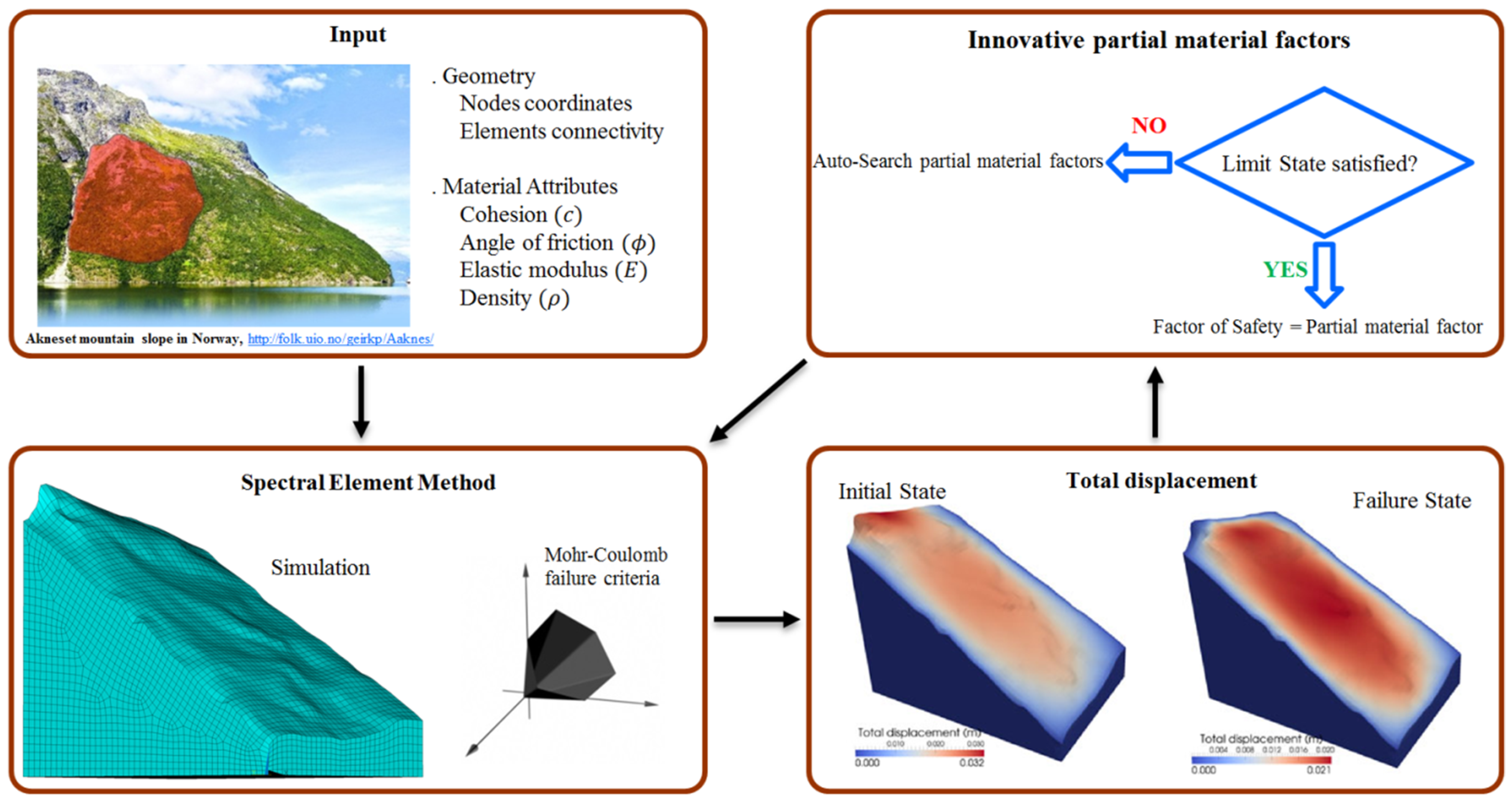
Figure 4.
Flowchart of the interaction between SEM and SRF.

Figure 5.
Schematic convergence to the design trigger (DT) within two iterations; for State 2 in Figure 4. (a) Initial (old) analysis and (b) updated (new) analysis.
Figure 5.
Schematic convergence to the design trigger (DT) within two iterations; for State 2 in Figure 4. (a) Initial (old) analysis and (b) updated (new) analysis.
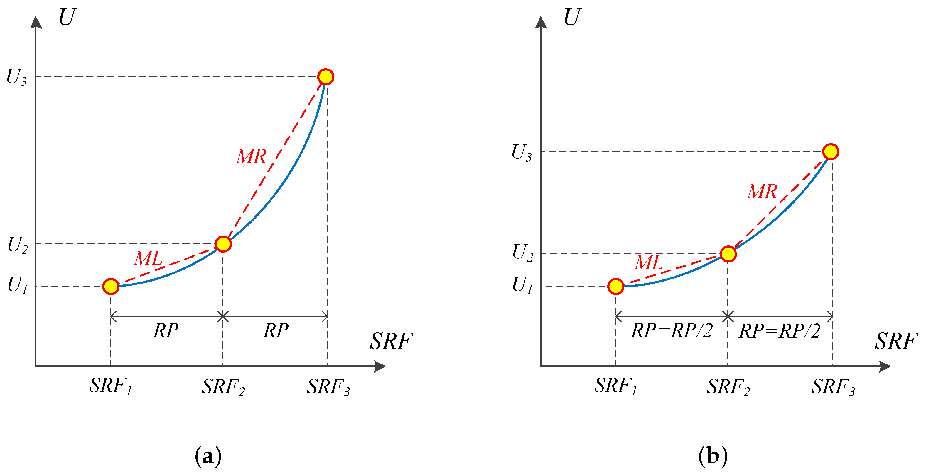
Figure 6.
Generic discretized model of the case studies. (a) Applied boundary conditions, (b) Case 1 and (c) Cases 2 and 3.
Figure 6.
Generic discretized model of the case studies. (a) Applied boundary conditions, (b) Case 1 and (c) Cases 2 and 3.

Figure 7.
Determination of the SF based on the maximum displacement and relevant gradient diagrams. (a) Case 1, displacement, (b) Case 1, gradient, (c) Case 2, displacement, (d) Case 2, gradient, (e) Case 3, displacement, and (f) Case 3, gradient.
Figure 7.
Determination of the SF based on the maximum displacement and relevant gradient diagrams. (a) Case 1, displacement, (b) Case 1, gradient, (c) Case 2, displacement, (d) Case 2, gradient, (e) Case 3, displacement, and (f) Case 3, gradient.


Table 1.
Comparison of the safety factor for the three case studies using different techniques.
| Methods | Case 1 | Case 2 | Case 3 |
|---|---|---|---|
| Xing [32] | 2.122 | 1.553 | 1.441 |
| Bishop’s modified method (Lam and Fredlund [31]) | - | 1.607 | 1.511 |
| Janbu’s simplified method (Lam and Fredlund [31]) | - | 1.558 | 1.481 |
| CLARA (Lam and Fredlund [31]) | - | 1.62 | 1.54 |
| CLE (Lam and Fredlund [31]) | - | 1.603 | 1.508 |
| Chen et al. [30] | 2.262 | 1.717 | - |
| Chen et al. [30] | 2.187 | 1.603 | - |
| FEM (Griffiths and Marquez [33]) | 2.17 | 1.58 | - |
| SEM (Gharti et al. [14]) | 2.18 | 1.57 | 1.49 |
| SEM (DT = 30%)—present study | 2.17 | 1.59 | 1.46 |
| SEM (DT = 50%)—present study | 2.18 | 1.61 | 1.48 |
| SEM (DT = 70%)—present study | 2.19 | 1.62 | 1.5 |
© 2019 by the authors. Licensee MDPI, Basel, Switzerland. This article is an open access article distributed under the terms and conditions of the Creative Commons Attribution (CC BY) license (http://creativecommons.org/licenses/by/4.0/).
Share and Cite
MDPI and ACS Style
Seyed-Kolbadi, S.M.; Sadoghi-Yazdi, J.; Hariri-Ardebili, M.A. An Improved Strength Reduction-Based Slope Stability Analysis. Geosciences 2019, 9, 55. https://doi.org/10.3390/geosciences9010055
AMA Style
Seyed-Kolbadi SM, Sadoghi-Yazdi J, Hariri-Ardebili MA. An Improved Strength Reduction-Based Slope Stability Analysis. Geosciences. 2019; 9(1):55. https://doi.org/10.3390/geosciences9010055
Chicago/Turabian StyleSeyed-Kolbadi, S. M., J. Sadoghi-Yazdi, and M. A. Hariri-Ardebili. 2019. "An Improved Strength Reduction-Based Slope Stability Analysis" Geosciences 9, no. 1: 55. https://doi.org/10.3390/geosciences9010055
Note that from the first issue of 2016, this journal uses article numbers instead of page numbers. See further details here.