Article

Monitoring Groundwater Change in California’s Central Valley Using Sentinel-1 and GRACE Observations

1
Jet Propulsion Laboratory, California Institute of Technology, Pasadena, CA 91109, USA
2
NASA Goddard Space Flight Center, Greenbelt, MD 20771, USA
3
Science Systems and Applications Inc., Lanham, MD 20706, USA
4
Global Institute for Water Security, University of Saskatchewan, Saskatoon, SK S7N 3H5, Canada
*
Author to whom correspondence should be addressed.
Geosciences 2019, 9(10), 436; https://doi.org/10.3390/geosciences9100436
Submission received: 14 September 2019 / Revised: 28 September 2019 / Accepted: 5 October 2019 / Published: 9 October 2019

Abstract

:
The San Joaquin Valley and Tulare basins in California’s Central Valley have intensive agricultural activity and groundwater demand that has caused significant subsidence and depletion of water resources in the past. We measured groundwater pumping-induced land subsidence in the southern Central Valley from March 2015 to May 2017 using Sentinel-1 interferometric synthetic aperture radar (InSAR) data. The InSAR measurements provided fine spatial details of subsidence patterns and displayed a superposition of secular and seasonal variations that were coherent across our study region and correlated with precipitation variability and changes in freshwater demand. Combining InSAR and Global Positioning System (GPS) data, precipitation, and in situ well records showed a broad scale slowdown/cessation of long term subsidence in the wetter winter of 2017, likely reflecting the collective response of the Central Valley aquifer system to heavier-than-usual precipitation. We observed a very good temporal correlation between the Gravity Recovery and Climate Experiment (GRACE) satellite groundwater anomaly (GWA) variation and long-term subsidence records, regardless of local hydrogeology and mechanical properties. This indicates the subsidence from satellite geodesy is a very useful indicator for tracking groundwater storage change. With the continuing acquisition of Sentinel-1 and other satellites, we anticipate decadal-scale subsidence records with a spatial resolution of tens to hundreds of meters will be available in the near future to be combined with basin-averaged GRACE measurements to improve our estimate of time-varying groundwater change.

1. Introduction

California’s Central Valley is one of the major agriculture regions in the United States. The urbanization and agricultural usage of water in the region rely heavily on groundwater resources. The southern part of the Central Valley (the San Joaquin Valley and Tulare Basin) is a broad alluvium-filled structural trough constituting the southern two-thirds of the Central Valley of California (Figure 1), where agricultural demands account for roughly 10% of the pumped groundwater in the United States [1]. The over-utilization of groundwater and periods of severe drought have caused a significant decline in groundwater levels over the past century [2], causing severe land subsidence [3].
The aquifer system of the Central Valley and in particular, the San Joaquin Valley and Tulare Basin, consists of alternating layers of coarse and fine material, creating a mix of confined, unconfined, and semi-confined units (Figure 2) [1]. Hydraulic conductivities in these materials range from about 3 × 10⁻⁶ to 1 × 10⁻⁷ m/day; elastic storage coefficients are around 1 × 10⁻⁵ m−1, and inelastic storage coefficients are about 1 × 10⁻⁴ m−1 [1,4]. Figure 2c shows the general hydraulic head and groundwater flow patterns in the Central Valley [1]. More recent maps, based on well measurements, can be found at the Groundwater Information Center website (https://gis.water.ca.gov/app/gicima/).
Subsidence affects the infrastructure and the flow capacity of water-conveyance systems, such as the California Aqueduct and flood-control canals, which exacerbates flood hazard and impedes the delivery of irrigation water [5]. Over pumping of groundwater also leads to an increase in aquifer contamination [6]. Inelastic (permanent) subsidence due to compaction in the subsurface aquifer system (mostly in aquitard layers) can cause permanent loss of aquifer storage capacity and affects sustainable groundwater usage [7].
Conventional monitoring of groundwater level change is through in situ measurements at observational wells, which are sparse, very cost ineffective, difficult to access, and a challenge for maintaining good quality control. Although the hydrology modeling may be capable of estimating groundwater level at a high spatiotemporal resolution, the conventional land surface models, such as Noah-MP [8], omit consideration of human activities, such as groundwater pumping, and so may underestimate the groundwater loss in the Central Valley [9]. Satellite observations from the Gravity Recovery and Climate Experiment (GRACE) satellite have been used to characterize the groundwater budget through the analysis of Earth’s gravity field (e.g., [10,11,12]) to estimate the basin-averaged groundwater storage change with time. Subsidence associated with groundwater depletion is also detectable from space, providing an indirect way to monitor groundwater level change.
The satellite interferometric synthetic aperture radar (InSAR) measures ground deformation at a spatial resolution of 10 to 100 s of meters and is increasingly used in mapping land subsidence and inferring hydrogeological properties (e.g., [7,13,14,15,16,17]). Conventionally it has been challenging to use C-band InSAR (wavelength ~5.6 cm) to measure land elevation change because of its radar backscatter decorrelation over several weeks in moderately vegetated areas (e.g., [18,19,20]). Past C-band SAR satellites, such as European Remote Sensing (ERS) and Envisat (“Environmental Satellite”) from the European Space Agency (ESA), were subject to severe temporal decorrelation due to irregular and infrequent acquisitions, which were limited by their 35-day repeat interval. Mapping subsidence in the Central Valley is more feasible for L-band InSAR, such as the Advanced Land Observing Satellite (ALOS) (e.g., [7,13,14]), thanks to its longer wavelength (~24 cm), which decorrelates more slowly in the presence of vegetation than shorter wavelength radars.
The C-band Sentinel-1 (S-1) SAR mission began operations in 2014 with a nominal repeat interval of 12 days, resulting in significantly improved temporal coherence. S-1’s continuous observations and free and open data policy allow the effective use of satellite remote sensing to map groundwater subsidence in the Central Valley. In this paper, we present results demonstrating the use of S-1 terrain observation by progressive scan (TOPS) data to measure surface subsidence change over part of the southern Central Valley from March 2015 to May 2017. We employ InSAR time series analysis to derive the deformation time history and compare it with in situ GPS. We also compare the InSAR-derived subsidence history with updated GRACE groundwater anomaly (GWA) estimates from 2011 to May 2017. Despite the scale differences, we show a very good temporal correlation between GRACE GWA and land subsidence variations. We combine InSAR measurements, regional precipitation, in situ well, and GPS to examine spatiotemporal variations of subsidence and how the land responds to groundwater level change due to changes in usage and climate variability. We discuss how the combination of regional groundwater storage variation from GRACE and InSAR-derived groundwater subsidence provides a cost-effective means to monitor groundwater change.

2. Materials and Methods

2.1. SAR Data and Interferometry Measurement

The Copernicus Sentinel-1 mission consists of two satellites (1A and 1B) that were launched in September 2014 and April 2016, respectively, by the European Space Agency (ESA). Both S-1A and S-1B have the same ground track coverage and a nominal acquisition interval of 12 days. Thanks to an orbital separation of 180 degrees (https://sentinel.esa.int/), Sentinel-1A and B provide a revisit time as short as 6 days from the same orbital direction for the region of interest. S-1 mainly operates in interferometric wide-swath (IW) mode. By employing the TOPS technique, the IW mode enables coverage of a large area with a good spatial resolution (range × azimuth: ~3 m × 22.6 m) (https://earth.esa.int/web/sentinel/technical-guides/sentinel-1-sar/products-algorithms/level-1/single-look-complex/interferometric-wide-swath). For this study, we used S-1 data from descending track 42 from 2015/03/01 to 2017/05/13 (Table 1). Two frames of track 42 covering the coast range and about half of the San Joaquin Valley and part of the Tulare Basin (Figure 1) were used in the analysis.
We used the JPL/Caltech InSAR Scientific Computing Environment (ISCE) software to process the Sentinel-1 TOPS data. The stack processor for S-1 data in ISCE was used to co-register all SAR images to the same master geometry. The S-1 stack processor employs an enhanced spectral diversity technique to estimate azimuth misregistration between single look complex (SLC) images in a stack sense, enabling achievement of high accuracy azimuth co-registration between SLC images for low coherence and/or long interval pairs. We used the 30 m Shuttle Radar Topography Mission digital elevation model (DEM) to remove the topography phase and a 90 m DEM for geocoding. We used an adaptive power spectrum filter to reduce phase noise and improve phase coherence [21]. The pixel spacing of S-1 data at full resolution is ~2.3 m × ~14.1 m in slant range and azimuth direction. To enhance phase coherency, we applied multi-looking factors of 33 and 11 in range and azimuth, respectively, resulting in pixel postings of ~76 m × 155 m in the range and azimuth, respectively. We unwrapped each interferogram using the statistical-cost, network-flow algorithm for phase unwrapping (SNAPHU) and minimum-cost flow algorithm [22]. After unwrapping we carefully examined each interferogram for possible unwrapping errors and corrected them if needed using the masks of connected components from SNAPHU. We then geocoded the unwrapped interferograms to the longitude and latitude grid with a ground posting of 90 m. To avoid stitching SLC products released by ESA that may originate from different versions of Instrument Processing Facility (IPF) software, we required that two frames on the same date must have the same IPF versions.
Interferometric measurements typically contain several noise sources, such as orbital error, atmosphere noise, ionosphere noise, and residual DEM error, in addition to surface deformation signals. For modern SAR satellites, such as Sentinel-1, the orbital error is minimal because of very good orbital control [23] and high precision orbits provided by ESA. For atmospheric noise and DEM errors, we considered them during the time series analysis. Ionosphere noise is wavelength and latitude dependent. For the C-band S-1 sensor, ionosphere noise is not as significant as L-band and appears mostly in ascending track data due to the local fly-over time [24]. Nevertheless, we assessed the potential ionospheric noise for the selected pairs by applying a range split-spectrum technique to estimate ionosphere noise on the interferogram [25,26]. We found that the interferometric phase was nearly identical after removing the estimated ionospheric phase (Figure S1). Therefore we neglected the ionosphere effect in our analysis. Figure 3 shows two typical IW mode interferograms from our study data set.

2.2. Multi-Temporal InSAR Time Series Analysis

We used a variant of the Small Baseline Subset InSAR time series inversion approach to solve for S-1 line-of-sight (LOS) displacement time series and mean velocity (e.g., [27,28]). In the approach, we jointly estimated residual DEM error and tectonic offset (if needed) along with LOS displacement at each date [29,30]. We used spatiotemporal filtering to remove high-frequency turbulent troposphere noise. For Sentinel-1, the perpendicular baseline (Bperp) varied from ~130 m to 150 m (Figure 4). The good orbital control significantly alleviated geometric decorrelation. The Central Valley is challenging for C-band interferometry because of low coherence associated with farming activity and vegetation coverage. To mitigate the temporal decorrelation, we only formed interferograms between a given date and its four closest neighbors in time. This resulted in 123 interferograms, the majority of which have time intervals of less than 24 days (Figure 4). The perpendicular baseline (Bperp) and time separations of these interferometric pairs are listed in Table S1.
To maximize the number of coherent pixels, we considered the pixels that have coherence >0.6 in at least 60% of the total number of the interferograms in our time series analysis. As shown in Figure 5, most pixels in our study area had coherence above the threshold. The increased coherent area is largely due to the small perpendicular baselines and short temporal separations of the interferograms. As InSAR measures relative LOS displacements between two acquisitions, to tie InSAR measurement to ground truth observations, we referenced each interferometric measurement to a region close to the GPS station P305 (See subsequent figure for the location), whose position time series showed the deformation in the reference area was steady over our study period (Figure S2).
The derived InSAR LOS displacement time series were validated against GPS time series at the same locations, projected to the S-1 LOS. We differentiated the GPS time series with regard to the GPS site (P305) located at the same location as the reference pixel used in the InSAR time series analysis. This removed the datum difference between the two data sets and ensured that the GPS time series were comparable to the InSAR measurements. Taking the differential positioning with regard to a stable region also helped remove common tectonic motions as interseismic tectonic motions are typically long wavelength and slowly varying in space. This facilitated the separation of non-tectonic groundwater-related deformation from tectonic sources.

2.3. GRACE Data Analysis

Satellite observations of time-variable gravity from the GRACE mission (e.g., [10,31]) provided a crucial component in estimating changes in water storage throughout the globe. Various recent studies have demonstrated that GRACE-derived estimates of variations of total water storage (TWS) can provide groundwater storage change estimates with sufficient accuracy [32,33,34]. TWS includes all the snow, ice, surface water, soil water, canopy water, and groundwater in a region, and when combined with auxiliary hydrological datasets, TWS can be utilized to infer process information on groundwater or other water sources. These GRACE-based methods have been applied to estimate rates of groundwater depletion in northern India [35,36], the Middle East [37,38], Northern China [39,40], California [10,11,12,34], among others. In this study, the JPL RL05M.1 Version 2 GRACE mascon product [41,42] was used to examine water storage changes in California’s Central Valley (~52,000 km2) and its underlying groundwater aquifer system during the GRACE satellite period, from April 2003 through June 2017. We employed a similar approach as in [10] to estimate the groundwater anomaly (GWA) characterized as equivalent water height averaged over the region of interest. We corrected the effects of surface water, soil moisture, snow water equivalent from the TWS estimate to obtain GWA (Figure S3). For more details about the method, we refer to [10]. We performed GWA analysis for the southern Central Valley surrounding the San Joaquin (SJ) basin and the Tulare basin (TU) (Figure 1). We estimated the GWA uncertainties by taking into account the uncertainties in TWS, soil moisture due to different North American Land Data Assimilation System models, and errors in snow water equivalent and surface water estimation.

2.4. Precipitation Data
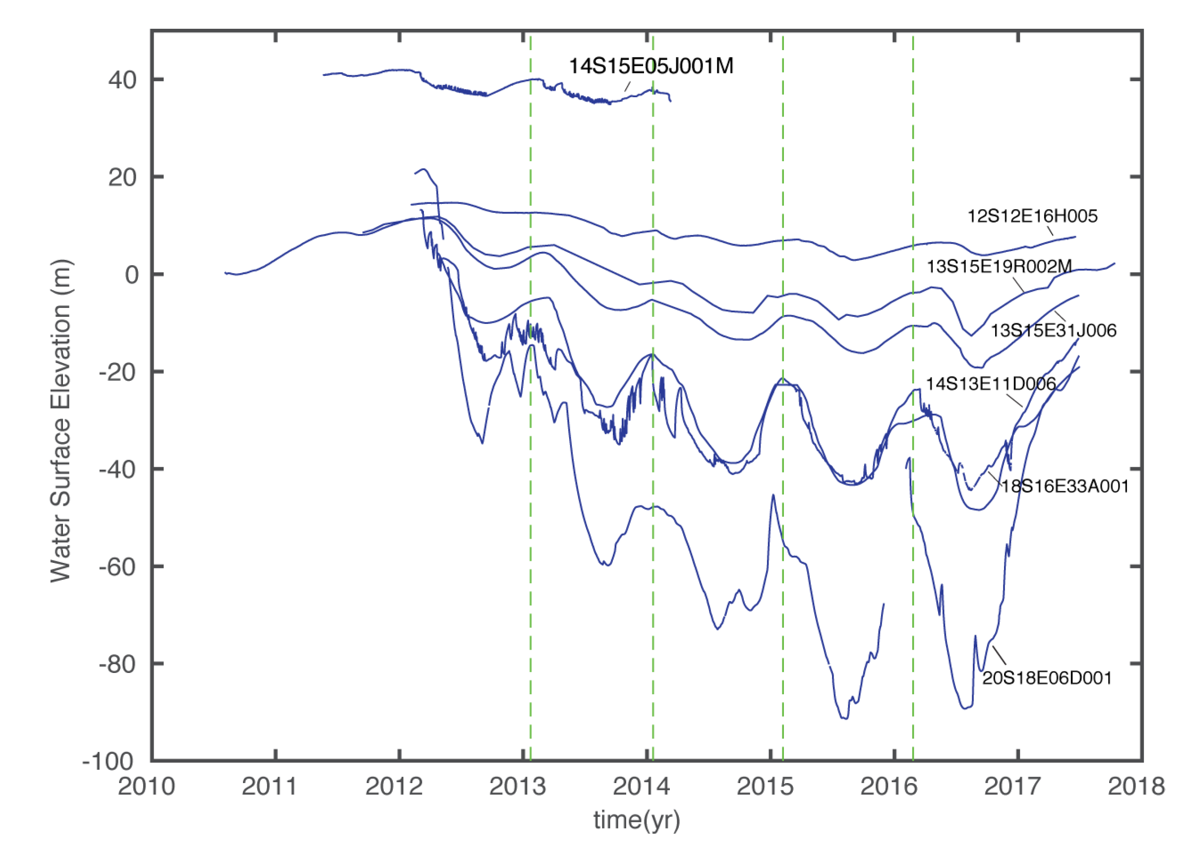
Precipitation data used in this study are from the Parameter-Elevation Regressions on Independent Slopes Model (PRISM) [43,44]. PRISM is a climate analysis system that uses point data, a digital elevation model (DEM), and other spatial datasets to generate gridded estimates of annual, monthly, and event-based climatic parameters. It has been designed to accommodate difficult climate mapping situations in innovative ways. These include vertical extrapolation of climate well beyond the lowest or highest station, reproducing gradients caused by rain shadows and coastal effects, and assessing the varying effects of terrain on precipitation. PRISM brings a unique combination of climatological and statistical concepts to the mapping of orographic precipitation. Figure 6 shows the spatially averaged PRISM precipitation data for the San Joaquin and Tulare basins and a combination of the two. The precipitation records show clear seasonal variations with more rainfall in winter and less in summer. The drought period of 2012–2016 was characterized by lower-than-normal rainfall followed by heavy winter precipitation of 2017, which concluded the drought.

2.5. Well Data

Water wells in the region are highly heterogeneous in space. Most wells have coarse and irregular temporal sampling. Wells that had continuous water level measurements throughout our study period were not common. We managed to identify and select the six most continuously monitored wells from the United States Geological Survey (USGS) National Water Information System (NWIS) (https://waterdata.usgs.gov/nwis/gw). These wells have continuous measurements of the depth to water surface (hydraulic head). We then converted these measurements to water surface elevation (WSE). The wells are relatively deep, with depths ranging from ~70 to ~414 m (Table S2). Figure 7 shows the WSE changes in the wells. The annual variation at these wells was synchronous with surface precipitation. The short-term variation was underlain by a longer-term trend of decrease in water level as a result of groundwater overdraft due to the 2012–2016 drought. Despite being at different depths and locations, the wells had simultaneous water level changes (both short- and long-term). There was no significant latency in water level change between different wells, suggesting they are well-connected beneath the surface and water recharge resulting from precipitation and/or correlated variation in pumping due to the availability of surface water affects the water level in a similar way regardless of their depth. The overall temporal change was consistent with cumulative surface precipitation variability.

3. Results

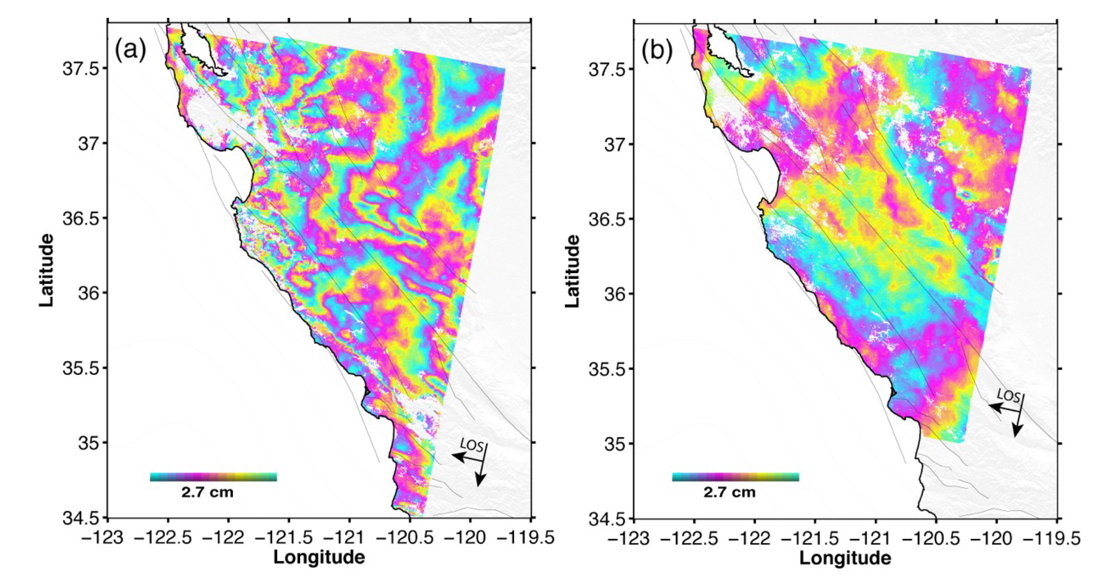
3.1. InSAR Mean LOS Velocity Map and Time Series Results

Figure 8 shows the mean velocity map along the LOS direction from the Sentinel-1 InSAR time series analysis. The differencing with regard to the stable reference location removed most slowly varying horizontal movement and makes the LOS displacements predominantly from vertical deformation. It is possible to combine ascending and descending tracks to estimate both horizontal and vertical components, but we leave that to a future study. If we assume the LOS rate is mainly due to vertical deformation, we can convert the LOS rate to a vertical subsidence rate by dividing the cosine of the nominal incidence angle. For the comparison of subsidence from difference SAR sensors over different periods, we convert the LOS displacement to vertical subsidence to remove geometry ambiguity. The subsidence map in 2015–2017 shows much higher subsidence rates than the previous drought period (2006–2010). For the selected profile, our estimated land subsidence rate reaches up to ~25 cm/year while the maximum subsidence rate derived from L-band ALOS data in 2006–2010 was ~14 cm/year (Figure 8b, Figure S4) [13]. Hereafter we separated the use of LOS subsidence and vertical subsidence but note that the former provides a good proxy of the latter as they can be converted to each other by some constant factors.
Note that the profiles of vertical deformation rates from both periods (Figure 8) have a maximum subsidence at about the same location (X = ~10 km, or ~120.35° W, 36.98° E) but the spatial extent of the subsidence in 2015–2017 appears to be much broader than that in 2006–2010 (Figure S4). For example, for a subsidence rate of ~5 cm/year, the width of the subsidence “bowl” was ~35 km as compared to ~24 km for 2006–2010. The recent subsidence map also reveals some new subsidence features that were absent during the previous drought period. For example, two small rapidly subsiding areas near Mendota and Tranquility and northwest of Kettleman City. The expanding spatial extent and increasing amplitude of previously mapped subsidence areas and emergent new subsidence features suggest the two consecutive drought periods (2006–2010 and 2012–2016) imposed enormous stress on the groundwater resource, exacerbating groundwater over-draft and leading to an increase in the area of the depletion around the pumping site and resultant subsidence.
Comparison between Sentinel-1 LOS displacement time series and co-located projected GPS LOS displacement time series at selected GPS sites showed very good agreement between the two (Figure 9). We used a three-component (east, north, up) GPS position time series solution in the North America reference frame from the Geodetic Laboratory at the University of Nevada, Reno (http://geodesy.unr.edu) in our analysis. We derived the differential GPS time series with regard to the reference station P305. The agreement between InSAR LOS displacement and in situ GPS data suggests that the Sentinel-1 InSAR captures the ground deformation accurately with an average root-mean-square (RMS) error of ~7 mm.
The LOS displacement time series of ~20 million pixels in the imaging area enabled us to examine the spatiotemporal pattern of the subsidence (Figure 10). For the time span covered by our analysis, the LOS subsidence time series at different locations showed very similar time-dependent behaviors (Figure 10a,b) that were characterized by a secular trend superimposed with short-term pause and resumption. To quantify how similar the deformation history was at different locations, we used the displacement time series at the pixel location collocated with the GPS station TRAN (lon. −120.25, lat. 36.65. http://geodesy.unr.edu/gps_timeseries/) as the representative time history of the regional subsidence. We performed temporal cross-correlation between the reference time series and the time series at all pixel locations over the entire image. This resulted in a correlation coefficient matrix that had the same dimension as the velocity map in Figure 10a. Each entry in the matrix represents the extent of temporal correlation between the subsidence displacement time series at that location and reference subsidence history. We chose a correlation threshold of 0.9 and mask out any pixel that had the cross-correlation below the threshold (Figure 10c,d). The resultant masked velocity map successfully captured all rapid subsidence areas, suggesting that the entire area covered by our Sentinel-1 InSAR data experienced very similar temporal subsidence history, consistent with the observation of similarity of the LOS time series at different locations in Figure 10b.
The co-located well 12S12E16H005 and GPS station ALTH (Figure 10a) provided a good opportunity to understand the complex temporal relationship between groundwater level change and corresponding surface deformation over a time span of more than 6 years. Figure 11 shows the comparison of the vertical subsidence time series at the GPS station ALTH and water level change at the well 12S12E16H005. The observed subsidence is characterized by a “secular” trend and “seasonal” variation that took place over several months. We found the WSE of the well displays a rapid drawdown during the 2012–2016 drought period. The multi-year decrease in groundwater level, in general, correlates well with the secular trend of the subsidence. The water level reached the lowest point at ~2015.7 (~Sept. 2015) (orange dashed line in Figure 11) then recovered after that. In comparison, the secular trend of land subsidence continued, reaching a maximum of ~25 cm (with regard to our reference date of 2012.1) at ~2016.8 (~Oct. 2016) (blue dashed line in Figure 11) right before the 2017 rainy season (see Figure 11). The secular subsidence largely ceased at the time of the 2017 winter season. The heavier-than-usual precipitation in the winter of 2017 introduced more recharge to the aquifers and a decreased need for pumping, causing a slight reversal of land subsidence (“uplift”) due to poroelastic rebound. The Central Valley includes a shallow unconfined aquifer and deeper confined aquifers [1]. The well has a depth of ~152 meters, deeper than the typical depth range of shallow aquifers in the Central Valley [1,11]. The observed elastic (seasonal) and inelastic (irreversible) deformation suggests that the well penetrates some confined aquifers and compacting aquitards (mostly clay layers). The secular deformation, as a result of fine-grained rearrangement in the compacting layer due to hydraulic head falling below the previous lowest level (pre-consolidation head), can lead to permanent loss of water storage capability [7]. This inelastic deformation due to aquitard compaction can continue due to slow equilibration even after the water level recovers. We found the time lag between the water level recovery and the subsidence cessation was about 1 year. Similar latency was also observed from the joint analysis of the GRACE GWA time series and the subsidence time history (see Section 3.3 for more details).

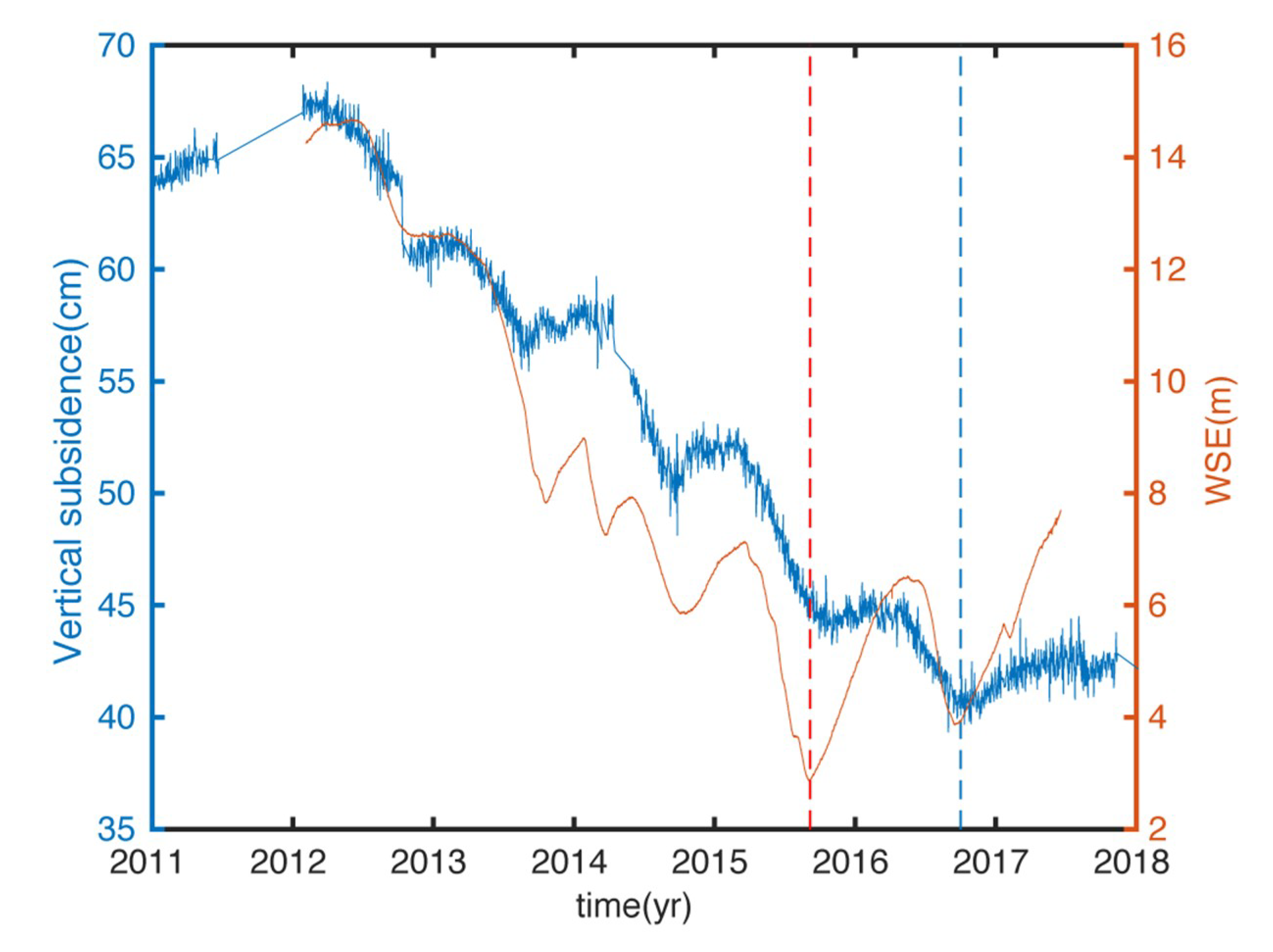
3.2. Broad Scale Slowdown of Secular Land Subsidence in Response to the Wetter Winter of 2017

Groundwater related subsidence signals in our study area shared very similar temporal behavior with annual oscillations superimposed on a secular trend that significantly slows down or ceased in the wetter winter of 2017. The oscillation was likely driven by elastic response of the embedded aquitard layers to the seasonal variation of water recharge and pumpage, while the secular trend represents the inelastic component of subsidence. Murray and Lohman [15] used Sentinel-1 data from another track further south in the southern San Joaquin Valley (SSJV) to report a similar slowdown in subsidence. The SSJV experienced large subsidence in the previous 2006–2010 drought, some of which was captured by other satellite SAR sensors, such as L-band ALOS-1 (Figure S5) [13]. We examined the time-dependent subsidence history in the SSJV using LOS subsidence time series from two selected GPS stations (CRCN, LEMA), both of which are located in the area experiencing severe subsidence in 2006–2010 (Figure S5). The results showed very similar temporal variation of the subsidence as station TRAN in our study area, indicating the slowdown of the subsidence was prevalent and may represent a broad-scale response of the Central Valley aquifer systems to the increased surface water availability and reduced groundwater demand. Note that residual compaction may still continue at some local areas even after the majority of the subsidence region stops subsiding [15].
Because of very similar regional history as imaged by both InSAR and GPS data (Figure 10b–e, Figure S5e,d), we used the LOS displacement time series at GPS station TRAN as the representation of regional temporal variation of subsidence and converted it to vertical subsidence to compare with the GRACE GWA estimate in the following analysis. The continuous GPS time series allowed a better characterization of the temporal relationship between GRACE GWA and land subsidence over a much longer time scale than the span of InSAR data, shedding insight into the relationship between these distinctive yet closely related observables.

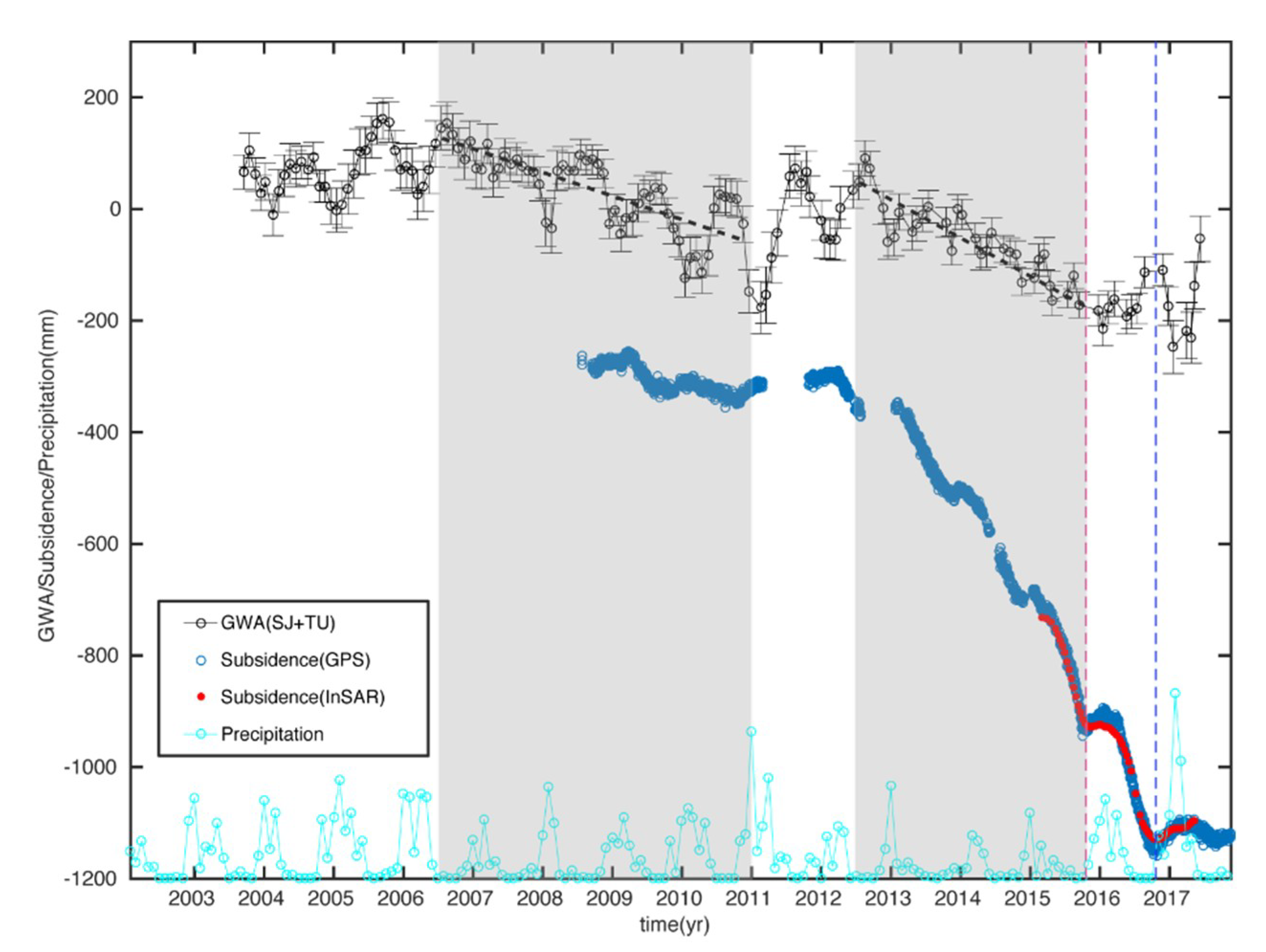
3.3. Comparison of GRACE Derived Groundwater Loss and Subsidence Time History

Figure 12 shows the comparison of GRACE-derived groundwater anomaly, representative subsidence time series, and monthly PRISM precipitation data. We considered the GWA change in the southern Central Valley. The analysis was conducted using GWA estimates from the San Joaquin Valley basin (SJ), Tulare basin (TU), and a combination of the two (SJ + TU). Both precipitation and GRACE GWA change showed that, during the drought periods of 2006–2010 and 2012–2016, there was a secular trend and seasonal variation of groundwater storage. The secular trend of GWA corresponded well with the secular trend of subsidence. Despite roughly comparable GWA changes, the average subsidence rate in 2012–2016 was much larger than that in 2006–2010, possibly because consecutive droughts and paucity of surface water put more dependence on groundwater for agriculture use during the most recent drought, exacerbating ground subsidence. On a basin scale, we noticed nearly the similar time lag between the recovery time of GWA and cessation of long-term subsidence (Figure 12) as the individual well (Figure 11), consistent with the view of a broad, coherent response of the SJV aquifer system to the wetter winter of 2017.
We found there was a strong correlation between GRACE derived GWA variation and measured ground subsidence. To quantify how sensitive the correlation is to the error distribution of the GWA, we estimated the uncertainties of correlation using a Monte Carlo simulation. A synthetic GWA time series was generated using the estimated GWA from SJ + TU with random noise added (assumed to be Gaussian with zero mean and the same variance as the real data). The synthetic data were then used to compute the correlation with ground subsidence, and we repeated this process for ~100,000 times, each time with different random noise added to the synthetic GWA time series. The resultant histogram of correlation is shown in Figure 13a. The estimated correlation with uncertainty was ~0.71 ± 0.03, suggesting the observed correlation is robust. Correlation with GWA from SJ or TU gave a very similar correlation coefficient. Since the subsidence uncertainties propagated from GPS position uncertainties were very small (a few mm), we neglected their effects in the simulation.
To test if the large correlation between GWA and subsidence was mainly due to secular or seasonal components of the subsidence, we performed a spline fit (order 4) to the subsidence time series to separate secular and seasonal components (Figure 13b,c). Separation of the two were robust and did not change much if we adopted different spline order. The seasonal variation showed clear time-varying amplitudes and suggests one needs to be cautious when fitting seasonal subsidence in the Central Valley using constant amplitude sinusoidal terms as assumed in previous studies (e.g., [15]). We computed the correlation coefficient between the GWA and secular and seasonal components, respectively, following the same procedure as described above (Figure 13d,e). Our results show the correlation coefficient between GWA and secular subsidence remained almost the same (~0.72 ± 0.03), while the correlation with the seasonal component was less significant (~0.14 ± 0.04). Our results suggest that the strong correlation between GWA and deformation time series was dominated by secular subsidence signals. We tested our results using different GPS stations with longer time series across the basin (Table 2) and found the general conclusion held regardless of hydrogeology, pumping, and mechanical property at each location. These results suggest a good portion of the observed GRACE GWA change must reflect water loss due to inelastic compaction in the aquitard layers. This is in contrast to some previous studies, such as [11], which assume all the groundwater change as measured by the GRACE GWA is from the shallow unconfined aquifer, which does not produce significant inelastic deformation.

4. Discussion

The very good temporal correlation between basin-wide GRACE GWA and subsidence over longer time scales suggests that subsidence signals are a very useful indicator for monitoring the state of groundwater. The integrated use of GRACE, subsidence, and in situ well data provides important information about what is happening in the Central Valley aquifer system. Currently, the long time-span subsidence time series is limited to a sparse GPS network. The InSAR satellites, such as C-band Sentinel-1 and L-band ALOS-2 (with a repeat time of 14-days), have been in operation since 2014. The L-band ALOS-4 and NASA-ISRO SAR (NISAR) mission will be launched in 2021 and 2022, respectively. We anticipate that the continuing operation of the existing satellites into the foreseeable future, along with forthcoming new satellites, will drastically change ways to map land elevation change and enable us to map time-varying groundwater deformation signals at 10 to 100 s of meters over decades, similar to GPS.
The latency between groundwater recovery and the cessation of inelastic subsidence represents a residual compaction effect due to the delayed equilibration of aquitard head levels. The concurrent change between subsidence and water level change before groundwater recovers suggests that the delayed deformation occurred during our study period and was not due to the effects of historical pumping (Figure 11). If we assume the compacting aquitard layer equilibrates with aquifer layers above and below it, the delay can be approximated by the following equation [7,45]:
τ ( b 0 v 2 ) 2 S s k v K v ,
where S s k v is inelastic skeletal-specific storage, K v is vertical hydraulic conductivity, and b 0 v is the thickness of fine grained, aquitard layers (mostly clay) that experience inelastic compaction. The K v S s k v is also termed the diffusivity ( D v We can estimate b 0 v if we know the S s k v and K v or D v . If we take the average diffusivity 1.32 × 10⁻³ m2/d as determined from previous studies [4,7], we estimate b 0 v is ~1.4 m. Note that this estimate reflects the integrative portion of the fine-grained clay layers that experienced compaction and should not be regarded as the total clay layer thickness. Interestingly, the time lags from the GRACE basin scale average (Figure 12) and at the location of GPS station ALTH (Figure 11) had similar values, suggesting that compaction occurs in a broad area and the subsidence in our study period is mostly permanent.
Land subsidence from groundwater pumping is a function of subsurface hydrogeology, which is typically poorly known. While InSAR measures ground subsidence at fine spatial resolution, GRACE GWA estimation presents a bulk estimate of groundwater change averaged over a footprint of ~52,000 km3. It is intriguing to observe the good temporal correlation between GRACE GWA and long-term subsidence change, as shown by InSAR and GPS in our study region, regardless of local geological conditions (Table 2). The long-term subsidence is likely the result of water loss due to compaction of compressible fine-grained layers (“water of compaction”) in the aquifer system [46]. Faunt et al. [47] combined hydrologic modeling with well and subsidence data to show that most subsidence in the 2012–2016 drought was permanent. Smith et al. [7] suggested that the vast majority of subsidence in southern San Joaquin Valley in the 2006–2010 drought was permanent, leading to the loss of groundwater storage capability. The GRACE-derived GWA time series shows a long-term groundwater volume decrease during drought periods (Figure 12). There was some recovery following the 2006–2010 drought. But such recovery was short-lived due to the subsequent 2012–2016 drought. The good correlation between GWA and subsidence is determined mainly by their long-term trends, implying secular GWA decrease was likely permanent. If water level change is affected by the shallow unconfined and deep confined aquifer systems, several hypotheses may be incurred to explain the correlation: (1) the shallow unconfined portion of the Central Valley aquifer system contributes to the similar longer-term trend of water storage decrease but does not contribute much to detectable surface deformation; (2) large portions of the estimated GRACE GWA change, especially its long term trend over the drought periods, are mainly caused by water loss due to aquitard compaction. Testing the first hypothesis would require continuous monitoring of well water level and GRACE observations to see if sustained normal or above-normal precipitation will cause the recovery of GRACE GWA to the pre-drought level. Alternatively, if the large portion of GWA is due to water loss from irreversible compaction, we can downscale GRACE GWA, informed by InSAR subsidence patterns, to improve the spatial resolution of groundwater volume change. The latter will be crucial for local and regional water management. Combining GRACE measurements with InSAR derived subsidence has been attempted by Castellazzi et al. in Central Mexico and show the promise to integrate the complementary information of the two for improved groundwater depletion estimates [48].

5. Conclusions

Our joint analysis of GRACE GWA, land subsidence from Sentinel-1 InSAR and GPS, regional precipitation records, and in situ continuous well data depicted a consistent picture of groundwater storage change in the southern parts of the Central Valley. Our InSAR results showed similar subsidence time histories among different locations in the subsiding areas attested by a strong correlation between them. The temporal history of subsidence was characterized by a secular (inelastic) trend with short-term (elastic) variations modulated by seasonal precipitation. The seasonal components were in phase with surface precipitation and well water levels and likely affected by the shallow aquifer. The long-term subsidence was more likely related to the compaction of fine-grained aquitard layers within the aquifer system, which we found has time lag from elastic counterparts at the end of 2015 when the drought period ends. The long-term subsidence showed clear slowdown/cessation in the winter of 2016–2017, the second wettest rainy season on record. Similar behaviors were also found in other parts of the southern Central Valley by previous studies, suggesting it was more widespread and likely reflect a basin-wide response of a compacting aquifer system to the increase in water recharge and decrease in groundwater pumping. We found that the temporal change in GRACE GWA and ground subsidence on a longer time scale was highly correlated, regardless of local hydrogeology. This highlights that land subsidence, as measured by satellite remote sensing, can be a very useful indicator for monitoring groundwater storage change. It also suggests potentially these two can be combined for improved groundwater storage estimates at fine resolution.

Supplementary Materials

The following are available online at https://www.mdpi.com/2076-3263/9/10/436/s1, Figure S1: Example of interferograms after ionosphere noise correction and estimated ionosphere phase, Figure S2: The 3-component GPS position time series at station P305, Figure S3: Example of GRACE derived total water storage (TWS) change, groundwater anomaly, estimates of snow water equivalent, soil moisture, and surface water anomaly for the entire Central Valley, Figure S4: Mean LOS velocity map in 2006-2010 from L-band ALOS-1 ascending track 219 covering roughly the same area as Sentinel-1 data used in this study and selected velocity profile, Figure S5: Mean LOS velocity in 2006–2010 from ALOS-1 ascending track 218 in southern San Joaquin Valley basin, south of the Sentinel-1 track used in this study. LOS subsidence time series at GPS stations LEMA and CRCN and corresponding histogram of temporal correlation between GRACE GWA and subsidence time series at these stations, Table S1: S1 raw data list, perpendicular baseline, time separation, Table S2: Continuous wells’ IDs, longitudes, latitudes, and depths.

Author Contributions

Z.L. carried out the study and led the writing of the original draft of the paper. E.M. helped with the development of conceptualization. P.-W.L. performed the analysis of GRACE and precipitation data. E.M. and P.-W.L. contributed to the writing of the GRACE and Precipitation section. P.L. and T.G.F. provided support to the InSAR and well data analysis. J.S.F. supported GRACE data analysis. All authors co-edited and reviewed the manuscript.

Funding

The research described in this paper was performed under a contract with the National Aeronautics and Space Administration at the Jet Propulsion Laboratory, California Institute of Technology, and was also partly funded by the CA Department of Water Resources.

Acknowledgments

We thank the European Space Agency (ESA) for making Sentinel-1 data available for public access. Copernicus Sentinel data 2015–2017. Retrieved from ASF DAAC July 29, 2017, processed by ESA.

Conflicts of Interest

The authors declare no conflict of interest.

Abbreviations

The following acronyms are used in this paper:
ALOSAdvanced Land Observing Satellite
DEMDigital Elevation Model
ESAEuropean Space Agency
GWAGroundwater Water Anomaly
GRACEGravity Recovery and Climate Experiment
InSARInterferometric Synthetic Aperture Radar
IPFInstrument Processing Facility
ISCEInSAR Scientific Computing Environment
IWInterferometric Wide-swath
LOSLine-Of-Sight
NISARNASA-ISRO SAR
NWISNational Water Information System
PRISMParameter-Elevation Regressions on Independent Slopes Model
S-1Sentinel-1
SLCSingle Look Complex
SJSan Joaquin basin
SSJVSouthern San Joaquin Valley
SARSynthetic Aperture Radar
TOPSTerrain Observation with Progressive Scan
TUTulare basin
TWSTotal Water Storage
WSEWater Surface Elevation

References

  1. Faunt, C.C. Groundwater Availability of the Central Valley Aquifer, California; U.S. Geological Survey Professional Paper 1766; U.S. Geological Survey: Reston, VA, USA, 2009; p. 173.
  2. Diffenbaugh, N.S.; Swain, D.L.; Touma, D. Anthropogenic warming has increased drought risk in California. Proc. Natl. Acad. Sci. USA 2015, 112, 3931–3936. [Google Scholar] [CrossRef] [PubMed] [Green Version]
  3. Galloway, D.; Riley, F.S. San Joaquin Valley, California: Largest human alteration of the Earth’s surface. U.S. Geol. Surv. Circ. 1999, 1182, 23–34. [Google Scholar]
  4. Sneed, M. Hydraulic and Mechanical Properties Affecting Ground-Water Flow And Aquifer-System Compaction, San Joaquin Valley, California; U.S. Geologic Survey Open-File Report. 01–35; U.S. Geologic Survey: Reston, VR, USA, 2001; pp. 1–26.
  5. Sneed, M.; Brandt, J.T. Land subsidence in the San Joaquin Valley, California, USA, 2007–2014. In Proceedings of the International Association of Hydrological Sciences, Koblenz, Germany, 13–16 October 2015; pp. 23–27. [Google Scholar]
  6. Smith, R.; Knight, R.; Fendorf, S. Overpumping leads to California groundwater arsenic threat. Nat. Commun. 2018, 9, 2089. [Google Scholar] [CrossRef] [PubMed]
  7. Smith, R.G.; Knight, R.; Chen, J.; Reeves, J.A.; Zebker, H.A.; Farr, T.; Liu, Z. Estimating the permanent loss of groundwater storage in the southern San Joaquin Valley, California. Water Resour. Res. 2017, 53, 2133–2148. [Google Scholar] [CrossRef]
  8. Yang, Z.-L.; Niu, G.-Y.; Mitchell, K.E.; Chen, F.; Ek, M.B.; Barlage, M.; Longuevergne, L.; Manning, K.; Niyogi, D.; Tewari, M.; et al. The community Noah land surface model with multiparameterization options (Noah-MP): 2. Evaluation over global river basins. J. Geophys. Res. 2011, 116, D12110. [Google Scholar] [CrossRef]
  9. He, X.; Wada, Y.; Wanders, N.; Sheffield, J. Intensification of hydrological drought in California by human water management. Geophys. Res. Lett. 2017, 44, 1777–1785. [Google Scholar] [CrossRef] [Green Version]
  10. Lo, M.-H.; Ho, S.L.; Bethune, J.; Syed, T.H.; Swenson, S.C.; De Linage, C.R.; Rodell, M.; Famiglietti, J.S.; Anderson, K.J. Satellites measure recent rates of groundwater depletion in California’s Central Valley. Geophys. Res. Lett. 2011, 38. [Google Scholar] [CrossRef]
  11. Scanlon, B.R.; Longuevergne, L.; Long, D. Ground referencing GRACE satellite estimates of groundwater storage changes in the California Central Valley, USA. Water Resour. Res. 2012, 48, W04520. [Google Scholar] [CrossRef]
  12. Xiao, M.; Koppa, A.; Mekonnen, Z.; Pagán, B.R.; Zhan, S.; Cao, Q.; Aierken, A.; Lee, H.; Lettenmaier, D.P. How much groundwater did California’s Central Valley lose during the 2012–2016 drought? Geophys. Res. Lett. 2017, 44, 4872–4879. [Google Scholar] [CrossRef]
  13. Farr, T.G.; Liu, Z. Monitoring subsidence associated with groundwater dynamics in the Central Valley of California using interferometric radar. In Remote Sensing of the Terrestrial Water Cycle; Lakshmi, V., Alsdorf, D., Anderson, M., Eds.; American Geophysical Union: Washington, DC, USA, 2015; Volume 206, pp. 397–406. [Google Scholar]
  14. Ojha, C.; Shirzaei, M.; Werth, S.; Argus, D.F.; Farr, T.G. Sustained groundwater loss in California’s Central Valley exacerbated by intense drought periods. Water Resour. Res. 2018, 54, 4449–4460. [Google Scholar] [CrossRef]
  15. Murray, K.D.; Lohman, R.B. Short-lived pause in Central California subsidence after heavy winter precipitation of 2017. Sci. Adv. 2018, 4, eaar8144. [Google Scholar] [CrossRef] [PubMed] [Green Version]
  16. Rosi, A.; Tofani, V.; Agostini, A.; Tanteri, L.; Stefanelli, C.T.; Catani, F.; Casagli, N. Subsidence mapping at regional scale using persistent scatters interferometry (PSI): The case of Tuscany region (Italy). Int. J. Appl. Earth Obs. Geoinform. 2016, 52, 328–337. [Google Scholar] [CrossRef]
  17. Soldato, D.; Farolfi, G.; Rosi, A.; Raspini, F.; Casagli, N. Subsidence evolution of the Firenze-Prato-Pistoia plain (Central Italy) combining PSI and GNSS data. Remote Sens. 2018, 10, 1146. [Google Scholar] [CrossRef]
  18. Solari, L.; Del Soldato, M.; Bianchini, S.; Ciampalini, A.; Ezquerro, P.; Montalti, R.; Raspini, F.; Moretti, S. From ERS ½ to Sentinel-1: Subsidence monitoring in Italy in the last two decades. Front. Earth Sci. 2018, 6, 149. [Google Scholar] [CrossRef]
  19. Raspini, F.; Bianchini, S.; Ciampalini, A.; Del Soldato, M.; Solari, L.; Novali, F.; Del Conte, S.; Rucci, A.; Ferretti, A.; Casagli, N. Continuous, semi-automatic monitoring of ground deformation using Sentinel-1 satellites. Sci. Rep. 2017, 8, 7253. [Google Scholar] [CrossRef] [PubMed]
  20. Crosetto, M.; Monserrat, O.; Cuevas, M.; Crippa, B. Spaceborne Differential SAR Interferometry: Data Analysis Tools for Deformation Measurement. Remote. Sens. 2011, 3, 305–318. [Google Scholar] [CrossRef] [Green Version]
  21. Goldstein, R.M.; Werner, C.L. Radar interferogram filtering for geophysical applications. Geophys. Res. Lett. 1998, 25, 4035–4038. [Google Scholar] [CrossRef] [Green Version]
  22. Chen, C.W.; Zebker, H.A. Two-dimensional phase unwrapping with use of statistical models for cost functions in non-linear optimization. J. Opt. Soc. Am. 2001, 18, 338–351. [Google Scholar] [CrossRef]
  23. Fattahi, H.; Amelung, F. InSAR uncertainty due to orbital errors. Geophys. J. Int. 2014, 199, 549–560. [Google Scholar] [CrossRef] [Green Version]
  24. Liang, C.; Agram, P.; Simons, M.; Fielding, E.J. Ionospheric correction of InSAR time series analysis of C-band Sentinel-1 TOPS Data. IEEE Trans. Geosci. Remote. Sens. 2019, 57, 6755–6773. [Google Scholar] [CrossRef]
  25. Liang, C.; Fielding, E.J. Measuring azimuth deformation with L-Band ALOS-2 ScanSAR interferometry. IEEE Trans. Geosci. Remote. Sens. 2017, 55, 1–14. [Google Scholar] [CrossRef]
  26. Liang, C.; Liu, Z.; Fielding, E.J.; Burgmann, R. InSAR time series analysis of L-Band Wide-Swath SAR data acquired by ALOS-2. IEEE Trans. Geosci. Remote. Sens. 2018, 56, 4492–4506. [Google Scholar] [CrossRef]
  27. Berardino, P.; Fornaro, G.; Lanari, R.; Sansosti, E. A new algorithm for monitoring localized deformation phenomena based on small baseline differential SAR interferograms. IEEE Int. Geosci. Remote Sens. Symp. 2002, 2, 2375–2383. [Google Scholar] [CrossRef]
  28. Sansosti, E.; Casu, F.; Manzo, M.; Lanari, R. Space-borne radar interferometry techniques for the generation of deformation time series: An advanced tool for Earth’s surface displacement analysis. Geophys. Res. Lett. 2010, 37, 1–9. [Google Scholar] [CrossRef]
  29. Samsonov, S. Topographic Correction for ALOS PALSAR Interferometry. IEEE Trans. Geosci. Remote. Sens. 2010, 48, 3020–3027. [Google Scholar] [CrossRef]
  30. Liu, Z.; Lundgren, P.; Shen, Z. Improved imaging of Southern California crustal deformation using InSAR and GPS. In Proceedings of the 2014 SCEC Annual Meeting, Palm Springs, CA, USA, 6–10 September 2014. [Google Scholar]
  31. Tapley, B.D.; Bettadpur, S.; Ries, J.C.; Thompson, P.F.; Watkins, M.M. GRACE Measurements of Mass Variability in the Earth System. Science 2004, 305, 503–505. [Google Scholar] [CrossRef] [PubMed] [Green Version]
  32. Swenson, S.C.; Rodell, M.; Yeh, P.J.-F.; Famiglietti, J.S. Remote sensing of groundwater storage changes in Illinois using the Gravity Recovery and Climate Experiment (GRACE). Water Resour. Res. 2006, 42. [Google Scholar] [CrossRef]
  33. Zaitchik, B.F.; Rodell, M.; Reichle, R.H. Assimilation of GRACE Terrestrial Water Storage Data into a Land Surface Model: Results for the Mississippi River Basin. J. Hydrometeorol. 2008, 9, 535–548. [Google Scholar] [CrossRef]
  34. Massoud, E.C.; Purdy, A.J.; Miro, M.E.; Famiglietti, J.S. Projecting groundwater storage changes in California’s Central Valley. Sci. Res. 2018, 8, 12917. [Google Scholar] [CrossRef]
  35. Rodell, M.; Velicogna, I.; Famiglietti, J.S. Satellite-based estimates of groundwater depletion in India. Nature 2009, 460, 999–1002. [Google Scholar] [CrossRef] [Green Version]
  36. Tiwari, V.M.; Wahr, J.; Swenson, S. Dwindling groundwater resources in northern India, from satellite gravity observations. Geophys. Res. Lett. 2009, 36, L18401. [Google Scholar] [CrossRef]
  37. Voss, K.A.; Famiglietti, J.S.; Lo, M.-H.; Linage, C.; Rodell, M.; Swenson, S.C. Groundwater depletion in the Middle East from GRACE with implications for transboundary water management in the Tigris-Euphrates-Western Iran region. Water Resour. Res. 2013, 49, 904–914. [Google Scholar] [CrossRef] [PubMed] [Green Version]
  38. Forootan, E.; Rietbroek, R.; Kusche, J.; Sharifi, M.; Awange, J.; Schmidt, M.; Omondi, P.; Famiglietti, J.; Awange, J. Separation of large scale water storage patterns over Iran using GRACE, altimetry and hydrological data. Remote. Sens. Environ. 2014, 140, 580–595. [Google Scholar] [CrossRef]
  39. Moiwo, J.; Yang, Y.; Li, H.; Han, S.; Hu, Y. Comparison of GRACE with in situ hydrological measurement data shows storage depletion in Hai River basin, Northern China. Water SA 2009, 35, 663–670. [Google Scholar] [CrossRef]
  40. Feng, W.; Zhong, M.; Lemoine, J.-M.; Biancale, R.; Hsu, H.-T.; Xia, J. Evaluation of groundwater depletion in North China using the Gravity Recovery and Climate Experiment (GRACE) data and ground-based measurements. Water Resour. Res. 2013, 49, 2110–2118. [Google Scholar] [CrossRef]
  41. Wiese, D.N.; Yuan, D.-N.; Boening, C.; Landerer, F.W.; Watkins, M.M. JPL Grace Mascon Ocean, Ice, and Hydrology Equivalent Water Height RL05M.1 CRI Filtered Version 2, PO.DAAC, CA, USA. Available online: https://podaac-tools.jpl.nasa.gov/drive/files/allData/tellus/L3/mascon/RL05 (accessed on 30 September 2017).
  42. Watkins, M.M.; Wiese, D.N.; Yuan, D.-N.; Boening, C.; Landerer, F.W. Improved methods for observing Earth’s time variable mass distribution with GRACE using spherical cap mascons. J. Geophys. Res. Solid Earth 2015, 120, 2648–2671. [Google Scholar] [CrossRef]
  43. Daly, C.; Neilson, R.P.; Phillips, D.L. A statistical-topographic model for mapping climatological precipitation over mountainous terrain. J. Appl. Meteorol. 1994, 33, 140–158. [Google Scholar] [CrossRef]
  44. Daly, C.; Halbleib, M.; Smith, J.I.; Gibson, W.P.; Doggett, M.K.; Taylor, G.H.; Curtis, J.; Pasteris, P.P. Physiographically sensitive mapping of climatological temperature and precipitation across the conterminous United States. Int. J. Clim. 2008, 28, 2031–2064. [Google Scholar] [CrossRef]
  45. Riley, F.S. Analysis of borehole extensometer data from central California. Int. Assoc. Sci. Hydrol. Publ. 1969, 89, 423–431. [Google Scholar]
  46. Galloway, D.L.; Jones, D.R.; Ingebritsen, S.E. Land Subsidence in the United States; U.S. Geological Survey: Reston, VA, USA, 1999; Volume 1182, pp. 1–177.
  47. Faunt, C.C.; Sneed, M.; Traum, J.; Brandt, J.T. Water availability and land subsidence in the Central Valley, California, USA. Hydrogeol. J. 2016, 24, 1–10. [Google Scholar] [CrossRef]
  48. Castellazzi, P.; Martel, R.; Rivera, A.; Huang, J.; Pavlic, G.; Calderhead, A.I.; Chaussard, E.; Garfias, J.; Salas, J.; Goran, P. Groundwater depletion in Central Mexico: Use of GRACE and InSAR to support water resources management. Water Resour. Res. 2016, 52, 5985–6003. [Google Scholar] [CrossRef]
Figure 1. Regional map of the Central Valley region in California with topography in color and shaded-relief. The black lines are the plate boundary fault system. The red line outlines the Central Valley basin. Blue lines represent the Tulare, San Joaquin, and Sacramento basins, including upper and lower Sacramento basins. The black box indicates the ground footprint of the Sentinel-1 descending track 42 used in the study.
Geosciences 09 00436 g001
Figure 2. (a) Geomorphic map of surficial units in the Central Valley. Note the extent of Corcoran Clay, a major confining unit. (b) Generalized hydrogeologic cross-section (A-A’ in (a)) indicating layers used in the United States Geological Survey (USGS) groundwater model of the San Joaquin Valley and the location of the Corcoran Clay. Figures from [1]. (c) The altitude of the unconfined part of the aquifer system and groundwater flow paths simulated for Spring 2000 by [1].
Geosciences 09 00436 g002
Figure 3. Selected Sentinel-1 interferometric wide-swath (IW) mode interferometry of two pairs: (a) 2017/04/07–2017/04/19; (b) 2016/04/12–2016/05/06. The unwrapped phase is rewrapped at 2π radian (corresponding to 2.7 cm) to better reveal phase (displacement) variation. Each fringe represents the surface displacement of 2.7cm along the satellite line-of-sight (LOS). Both images are dominated by atmosphere noise.
Geosciences 09 00436 g003
Figure 4. Temporal and spatial perpendicular baseline plot showing all the interferograms formed between the available SAR acquisition dates and used in our InSAR data analysis. The detailed list and spatial and temporal baselines are given in Table S1.
Geosciences 09 00436 g004
Figure 5. Map view of the number of pixels (in percentage) with coherence above the selected threshold 0.6 for all interferograms. This provides a good indication of the coherent area.
Geosciences 09 00436 g005
Figure 6. Precipitation records derived from Parameter-Elevation Regressions on Independent Slopes Model (PRISM) for the San Joaquin Valley (SJ) basin and Tulare (TU) basin and a combination of the two, showing seasonal variations. There is much higher precipitation in 2017 due to the second wettest rainy season on record.
Geosciences 09 00436 g006
Figure 7. Water surface elevation (WSE) changes at seven continuous wells. The well ID is indicated at the end of each WSE time series. The well locations are indicated in the subsequent Figure 10a. Green dashed lines highlight the concomitant nature of WSE changes among all wells.
Geosciences 09 00436 g007
Figure 8. (a) Mean interferometric synthetic aperture radar (InSAR) line-of-sight (LOS) subsidence map derived from Sentinel-1 data and (b) Comparison of average vertical subsidence rate from Sentinel-1 (black) and Advanced Land Observing Satellite-1 (ALOS-1) (blue) for the selected profile. The LOS subsidence map in (a) is re-wrapped at 8cm/year to show spatial details. The longitude and latitude of the maximum vertical subsidence in (b) are ~120.35° W, 36.98° E.
Geosciences 09 00436 g008
Figure 9. Comparison of InSAR time series and projected GPS LOS time series at selected GPS stations. The GPS LOS displacements are projected using 3-component position time series. The gray and red circles are the raw and filtered InSAR time series with atmosphere noise removed.
Geosciences 09 00436 g009
Figure 10. (a) Zoom-in view of LOS subsidence velocity overlaid with GPS stations and selected pixel location (A, B) (red triangles) and well locations (green circles). GPS station P305 is the reference location used in the InSAR time series analysis. (b) InSAR LOS time series from the selected pixel locations and GPS stations. (c) Masked temporal correlation coefficient where the correlation is above the selected threshold (0.9). (d) LOS subsidence velocity masked based on (c). All areas that undergo subsidence are captured, suggesting very similar subsidence time histories in the subsiding areas.
Geosciences 09 00436 g010
Figure 11. Comparison of vertical subsidence time series at GPS station ALTH (blue line, left axis) versus water surface elevation (WSE) at the co-located well 12S12E16H005 (orange line, right axis). The orange dashed line indicates the time when the water level starts to recover. The blue dashed line is the time that the secular subsidence ceases.
Geosciences 09 00436 g011
Figure 12. Comparison of the Gravity Recovery and Climate Experiment satellite (GRACE)-derived groundwater anomaly (GWA), representative vertical subsidence time history, and PRISM precipitation variation with time. The GWA from combined San Joaquin Valley Basin (SJ) and Tulare basin (TU) are plotted with associated uncertainties. GWA from SJ or TU has very similar temporal variation; thus is not shown for legibility. The semi-transparent gray shaded areas indicate 2006–2010 and 2012–2016 drought periods with GWA trending lines (black dashed), respectively. The vertical subsidence time series are derived from the LOS displacement time series at the location of TRAN (blue circles—GPS; red dots—InSAR). The magenta dashed line in late 2015 indicates the time when the GWA starts to recover due to increased surface precipitation and groundwater recharge or reduced pumping while the blue dashed line in late 2016 is the time of secular subsidence cessation.
Geosciences 09 00436 g012
Figure 13. (a) Histogram of temporal correlation between GRACE GWA time series in the San Joaquin Valley and Tulare Basin and representative subsidence time series at selected locations. The distribution of the correlation coefficient is realized through a Monte Carlo simulation by taking into account GRACE GWA uncertainties. This gives a sense of how sensitive the estimated correlation is to the error distribution of GWA. (b) Spline fit (red) to the subsidence time series (black). The red line represents the secular trend of subsidence. (c) The seasonal component of subsidence signals after subtracting the secular trend. (d,e) Histograms between GRACE GWA and secular and seasonal variation of subsidence signals, respectively. Note that the correlation coefficient for the secular component is much larger than that for the seasonal component.
Geosciences 09 00436 g013
Table 1. Sentinel-1 data used in the analysis.
SatelliteOrbit DirectionTrackFrame# of SAR Images# of Interferometry PairsTime SpanGround Resolution (in Geo-Coordinate)Incidence AngleHeading (Clockwise from the North)
S-1descending42469,4746312320150301–2017051390 m30.7°–45.9°190°
Table 2. Correlation between groundwater anomaly (GWA) and line-of-sight (LOS) subsidence (short-term and long-term).
StationsGWA vs. SubsidenceGWA vs. Secular Trend (Long-Term)GWA vs. Seasonal (Short-Term)
ALTH0.73 ± 0.030.73 ± 0.030.04 ± 0.04
TRAN0.71 ± 0.030.72 ± 0.030.14 ± 0.04
CHOW0.72 ± 0.040.72 ± 0.040 ± 0.04
LEMA0.71 ± 0.040.71 ± 0.040.24 ± 0.04
CRCN0.70 ± 0.040.70 ± 0.040.06 ± 0.04

