Innovative Monitoring Tools and Early Warning Systems for Risk Management: A Case Study


1
Dipartimento di Ingegneria e Architettura, University of Parma, Parco Area delle Scienze 181/a, 43124 Parma, Italy
2
ASE – Advanced Slope Engineering S.r.l., Parco Area delle Scienze 181/a, 43124 Parma, Italy
3
ANAS S.p.a., Via Monzambano 10, 00185 Rome, Italy
*
Author to whom correspondence should be addressed.
Geosciences 2019, 9(2), 62; https://doi.org/10.3390/geosciences9020062
Submission received: 22 December 2018
/
Revised: 14 January 2019
/
Accepted: 24 January 2019
/
Published: 29 January 2019
(This article belongs to the Special Issue Mountain Landslides: Monitoring, Modeling, and Mitigation)
Abstract
:During recent years, the availability of innovative monitoring instrumentation has been a fundamental component in the development of efficient and reliable early warning systems (EWS). In fact, the potential to achieve high sampling frequencies, together with automatic data transmission and elaboration are key features for a near-real time approach. This paper presents a case study located in Central Italy, where the realization of an important state route required a series of preliminary surveys. The monitoring system installed on site included manual inclinometers, automatic modular underground monitoring system (MUMS) inclinometers, piezometers, and geognostic surveys. In particular, data recorded by innovative instrumentation allowed for the detection of major slope displacements that ultimately led to the landslide collapse. The implementation of advanced tools, featuring remote and automatic procedures for data sampling and elaboration, played a key role in the critical event identification and prediction. In fact, thanks to displacement data recorded by the MUMS inclinometer, it was possible to forecast the slope failure that was later confirmed during the following site inspection. Additionally, a numerical analysis was performed to better understand the mechanical behavior of the slope, back-analyze the monitored event, and to assess the stability conditions of the area of interest.
1. Introduction
Within the landslides risk management framework, early warning systems (EWS) represent a relevant option, especially when structural measures are not able to fully guarantee the safety of areas interested by instability phenomena. Some of the several advantages linked to EWS include their fast, simple, and low-cost implementation and their environmental friendliness [1].
A wide number of definitions and characterizations are present in the literature. As defined by Medina-Cetina and Nadim, early warning systems are “monitoring devices designed to avoid, or at least to minimize, the impact imposed by a threat on humans, damage to property, the environment, or/and to more basic elements like livelihoods” [2]. According to another definition provided by UN-ISDR (United Nations International Strategy for Disaster Reduction), early warning systems should be designed to “empower individuals and communities threatened by hazards to act in sufficient time and in an appropriate manner to reduce the possibility of personal injury, loss of life and damage to property and the environment” [3]. Following these considerations, several studies provided a selection of common elements and components that should be included in EWS design and implementation [4,5,6,7]. These actions can be summarized as follows:
- Field monitoring system, able to acquire physical quantities related to the phenomenon and transmit them to the elaboration centre;
- Analysis and forecasting method, which describes the landslide evolution, predicts its behaviour, and identifies critical events on the basis of alert thresholds (if available);
- Warnings and dissemination of alert messages, to notify the relevant authorities about the forecasted critical event;
- Emergency plans and measures, to be activated on the basis of the forecasting results obtained by applying the numerical model.
Among these actions, it is of particular importance to guarantee a correct definition, calibration, and validation of the predictive model [8]. In fact, the consequences of false alarms and/or delayed communications could be extremely dangerous and should be avoided at all costs. This issue is strictly related to the choice of the monitoring system which best suits the forecasting model implemented. In particular, innovative monitoring tools able to achieve high sampling frequencies with automatic and remotely controlled procedures represent a significant improvement compared to traditional approaches. This is particularly notable for failure forecast methods, which significantly benefit from high frequency dataset in order to accurately represent the ongoing phenomenon [9,10]. In more recent times, there have been a significant number of studies and research concerning the application of these concepts to develop early warning systems, involving case studies featuring different monitoring approaches [11,12,13,14,15].
This paper presents an early warning system designed according to the guidelines previously mentioned. The EWS relies on automated inclinometer tools to record displacement data with high sampling frequency. Following their elaboration, results are processed by a specific routine aimed to identify significant variations of displacement velocity trend. The time of failure forecast procedure is activated and updated according to these results, coupled with an automatic process specifically developed to send an alert message to the authorities responsible for the monitoring.
2. Materials and Methods
2.1. Case Study Description
The case study presented in this paper is the monitoring of a landslide that persists on the construction site of a state road connecting the Adriatic and Tyrrhenian Seas, through Abruzzo and Molise regions (Figure 1). The realization of the road first started in the sixties and now the completion of the last 5.3 km is ongoing. The works have undergone several delays due to numerous landslides, the collapse of the viaduct Le Barche near the town of Bomba, and bureaucratic problems. As reported by Strade&Autostrade, the completion works have a total cost of 190,433 million euros for an estimated period of 30 months starting from December 2016 [16].
The area is located in an intermediate sector between Central Apennines, featuring carbonatic platforms, and Southern Apennines, characterized mainly by clayey and clayey-arenaceous deposits named Molise units [17]. The site is affected by the presence of several landslides in the western sector of the area of interest, showing fast kinematics and sliding surfaces between 8 and 10 m depths. Other instabilities are present also in the Eastern areas, involving the first meters of material (max 3–5 m) represented by eluvial colluvial deposits.
During preliminary surveys that anticipated the installation of modular underground monitoring system (MUMS), some instability events were recorded. Specifically, an inclinometer casing was interrupted at 8 m depth, with 40 cm of settlements of the surrounding soil. Moreover, two landslide bodies invaded an old railway line.
2.2. Monitoring and Early Warning System Composition
During the preliminary surveys, an innovative and remotely controlled monitoring system was installed on-site, featuring high sampling frequency and automated procedures for data recording and elaboration. In particular, MUMS (Modular Underground Monitoring System) instrumentation has been chosen as the monitoring system’s main technology due to its advantages.
MUMS is an innovative-patented device developed and produced by ASE S.r.l. (IT). The instrumentation is an array composed of different nodes (named Links) connected by a quadrupole electrical and an aramid fiber cable, forming an arbitrarily long chain [18,19]. The device can be equipped with 3D MEMS (Micro Electro-Mechanical Systems), electrolytic cell, piezometer, thermometer sensors, and electronic board. Chains are custom made, with a distance between sensors that can vary along the vertical according to the specific case. A dedicated ASE 801 Control Unit automatically queries each different Link through RS485 protocol at a specified frequency that could be modified according to monitoring needs. Data collected are stored locally on a memory unit and sent to the mainframe server at the elaboration centre, where they are stored in a dynamic MySQL database with a daily multilevel back-up system. Upon arrival on the central server, raw data are processed by a proprietary software and algorithm in order to return the physical monitored quantities (e.g., displacements, forces, pressures). An interactive web-platform represents the results through multi-parametric graphs. Additionally, the system can automatically send alert and alarm messages for the activation of proper safety measures.
For the failure forecasting model, in the EWS presented in this paper the inverse velocity method (IVM) was implemented [20]. This model relies on the consideration that the inverse of displacement velocity decreases with time during the accelerating phase of the landslide. Thus, the time of failure can be forecasted by locating the point where the line interpolating the monitoring data intercepts the x-axis, corresponding to a theoretical infinite velocity. During the years following its introduction, IVM has been widely analyzed and studied, and several back-analyses were carried out on case studies, in order to test its effectiveness [21,22,23,24].
In the present case, a total of six MUMS tools, specifically vertical arrays, were installed in different time periods (Table 1). Each array was equipped with Tilt Link HR 3D V, composed of 3D MEMS sensors and electrolytic cells.
This paper focuses on DT0014 inclinometer and the events taking place on March 2017.
DT0014 inclinometer was installed on November 18, 2016 and the following day was considered as the elaboration reference date. The sample period was set to 1 h, sending data to the elaboration center once a day. The borehole was filled with cement at the bottom for about 1 m, in order to fix the anchor to the stable portion, and with a mixture of bentonite for the remaining part of the vertical. The installation process required a couple of hours. The data logger was powered through 12 V lead-acid battery and 5 W solar panel.
The monitoring came to an end on March 13, 2017 due to excessive deformations.
3. Results
3.1. Monitoring System Results
During the monitored period, the automatic inclinometer identified a series of displacement variations involving the first 6 m of soil, as reported in Figure 2. Notably, the instrumentation showed two significant changes in displacement rate (Figure 3) starting from January 23, 2017 and March 7, 2017 respectively. The phenomenon led to the progressive breaking of the array. For this reason, the cumulative movements at the end of monitoring, reported in Figure 4b, are underestimated after February 27, 2017, while the local displacements recorded above 5.65 m depth could be considered as correct (Figure 4a).
MUMS inclinometer DT0014 became completely inactive on March 13, 2017. During the last days of monitoring, the failure forecast routine was activated several times through the automatic activation criterion. Consequently, an alert procedure was triggered reporting the ongoing event to those responsible of monitoring. The landslide event was positively identified after an on-site inspection, displaying a complex dynamic characterized by several failures and scarps, major and minor events, settlements and displacements. Figure 5 shows the area surrounding MUMS vertical array following the landslide event.
An in-depth check of the monitoring instrumentation conditions was carried out during the on-site inspection, reporting that all the traditional inclinometer casings were inaccessible due to excessive soil deformation. In particular, some vertical boreholes were drilled recently and never used, resulting in a loss of money and time. This example shows how the traditional instrumentation (manual inclinometer) is often not appropriate to interpret and describe a failure event. Even an IPI (In Place Inclinometer), located at the originally expected sliding surface depth, would have missed the most part of the failure. In this context, MUMS device has been the only instrumentation able to identify and document the landslide event, providing also a measure of its magnitude, thanks to its automated data acquisition processes.
3.2. Time of Failure Forecasting
Following the alert procedures activation, those responsible of monitoring received information about the node, depth, displacement typology, acceleration, date and time of failure prediction, together with two graphs for each sensor. Notably, the first one showed the inverse of velocity (expressed as day/mm) versus time, together with the index of linear regression, while the second reports the velocity (mm/day) versus time. The purpose of the figures is to help the decision maker in his final evaluation, which is always required.
By observing the graphs of the first alert (Figure 6 and Figure 7), two main pieces of information are available: the dataset is consistent (seven points for both links) and the indexes of linear regression show a reliable fitting, particularly for node 95 (R2 = 0.95779). The last point of node 95 dataset seems to slightly diverge from the linear trend evidenced by the previous ones, and its effect will be discussed below. The displacement rate is consistent (node 95 has a final velocity of 43 mm/day) and the average acceleration (lasted 7 h) ranges between 24 and 45 mm/day2. In particular, the displacement rate clearly indicates that a potentially dangerous phenomenon is going on, if compared to standard quantities recorded between the installation date and the end of February, which have a value of 0.093 mm/day and 0.025 mm/day, respectively. Finally, considering the distances between links, it is possible to state that the movement has not a single shear plane but instead a zone where different sliding surfaces are present. This could be assessed by observing the values of displacement rate and acceleration.
The second alert (Figure 8 and Figure 9) features a smaller dataset (five points) with good indexes of linear regression (0.88 and 0.92) related to local superficial displacements (node 99). The concavity that characterizes the last part of the dataset tends to a horizontal asymptote for both cases and this could be an index of a decelerating movement. The information obtained is only related to a single portion of the vertical (the superficial one) and indicates a dynamic that interests only the close proximity of the ground level, probably caused by the adjustment of soil after the failure occurred on March 08. The displacement rate is very high, confirming that the situation has not stabilized yet.
The third alert message (Figure 10) features five points, with , and an increasing concavity for cumulative movements at 3.2 m depth. This outcome should not be underestimated, even if associated with a single event. It probably does not indicate an actual collapse but highlights the predisposing factors for a subsequent event.
Finally, the fourth and last alert procedure (Figure 11) evidences the final collapse of the slope. It features five points, with . A particularly relevant piece of information about this event is the constant increasing of acceleration (i.e., the increasing concavity of the velocity vs time curve) that regards the last part of the dataset, resulting in 58 mm/day, which is the higher value registered for the whole period of monitoring. This result, even if associated with the cumulative displacements of a single point, should activate every risk management procedure necessary for the site.
3.3. Alert System Response
Thanks to the on-site inspection and a series of back analyses, it was possible to classify two main landslide events, occurring on March 08, 2017 between 20:32 and 21:32, and on March 13, 2017 between 13:56 and 14:56. The uncertainty concerning the exact time is related to the sampling period: The first value (for example 20:32) represents the last available instrumental reading characterized by a numerical value, while the second one (21:32) is the first reading returning an error code (i.e., the breaking of the instrumentation after landslide event). It should also be noted that the sampling period was set to 1 h, and data reached the elaboration center once a day, at 12:00.
MUMS EWS is designed to recognize false positives that may happen under certain conditions, specifically:
- < 0 (negative time of failure, i.e., date of collapse is in the past);
- > 0 & , where is the time of the last raw data available represented by a numerical value. In detail, the date of failure precedes the last instrumental data recorded, which is not returning an error (i.e., the sensor is working correctly).
- The activation of inverse velocity method does not imply an automatic alarm to the responsible of monitoring. This is validated through a series of preliminary analyses, in particular:
- The number of points in the dataset. The minimum dataset considered is composed by five points. If this value increases, it means that a consistent trend of data is fulfilling the activation criterion conditions;
- The correlation coefficient R2: The linear regression index points out the ability of the linear model to reproduce the observed data. Model is activated for R2 > 0.8. Higher values indicate an increasing confidence level;
- Nature of displacements (cumulative or Local). The algorithm analyses the number and the typology of alarms referring to the presence of cumulative, local, or both cumulative and local displacements;
- Number of alarms previously sent: this parameter verifies the presence of previous alarms occurred during the previous days and characterizes the so-defined “conditioned alarms”, i.e., alarms whose reliability is dependent on other alarms previously issued by the algorithm.
In this case, due to necessities related to electric power consumption and availability on-site, the monitoring system was set to send data once a day to the elaboration centre resulting in a “near real-time” approach. Because of this, a series of false alarms were identified since the date of predicted collapse was in the future, referring to the acceleration date, but in the past, referring to the transmission date and hour. This issue could be solved by implementing a process designed to send monitoring data as soon as they are sampled, thus allowing a real-time elaboration.
Table 2 reports the comparison between time of failure predictions and time of failure observed for alarm or conditioned alarm events. In particular, the time of failure prediction column reports the values obtained by the application of the forecasting model, while the observed Tf indicates the actual date and time of the collapse. Similarly, the theoretical warning time column represents the time between reception of the alert message and forecasted time of failure, while observed warning time takes as a reference the actual time of failure. The first activation (links 93 and 95) resulted in a very positive result, evaluating the time of failure, respectively, 3 h and 1 h later.
It should be underlined that the aim of the algorithm is not to be a perfect tool that identifies the day and hour of collapse to the very minute. Instead, it is intended to provide useful information about the potentially dangerous phenomena that are currently evolving and suggest a time period when the collapse should be expected and carefully monitored.
The first alert procedure gave a correct response, with a warning time of 10 h (time between the data transmission and elaboration and collapse) that could have been 19 h in the case of a real-time data transmission. The operator that received the notification assumed that the warning time was of 11 h (time between the data transmission and elaboration and predicted time of failure) which is very close to the observed one. After this event, two conditioned alarms were activated on March 09 at 12:00, predicting a possible collapse some hours later. This second alert procedure, like the following one (March 10 12:00), is quite difficult to evaluate, because it could refer to the collapse observed on March 08 or it could express the first symptoms of the following collapse, which occurred on March 13. In these cases, the information should be interpreted as “you just observed a collapse and something is still going on, so be careful and keep a close eye on the situation”.
Finally, the last alert procedure (conditioned alarm) was activated on March 13 at 12:00, forecasting a potential collapse 4 h later. A main landslide event was actually observed 3 h later, with the definitive breakout of all the instrumentations on-site. The forecasting error was of only 1 h providing, however, the necessary time for a risk management procedure activation.
3.4. Back-Analysis Outcomes
In this case study, the synergic application of activation criterion and inverse velocity method showed adequate performances. Nevertheless, could the algorithm work even better? A back-analysis has been performed in order to answer this question, investigating the results after the event (i.e., conditioned by the knowledge about date and hour of collapse). The back analysis was executed using a spreadsheet software and selecting the best dataset of cumulative displacements available for the application of failure forecast method. The process, summarized in the flow chart reported in Figure 12, started by investigating the datasets identified by the automatic algorithm. Next, they were iteratively expanded by adding data before and after the extreme points of the chosen dataset, in order to improve the time of failure prediction.
Table 3 shows the results of the back-analysis procedure for both events.
The landslide event that occurred on March 08 is clearly identified by three sensors placed at 2.5 m, 1.8 m, and 0 m depth, corresponding to links 93, 95, and 99, respectively. In particular, the datasets are composed by eight points for links 95 and 99 and 16 points for node 93. The acceleration dates are estimated during the night between March 7 and 8 (links 93 and 95) or the morning of March 08. Time of failure predictions are very consistent, with a mean estimation error of 24 min in advance. Combining the three pieces of information in a single representation (Figure 13) they lead to a consistent result where a collapse should be expected between 20:50 and 21:20 (collapse effectively observed between 20:32 and 21:32).
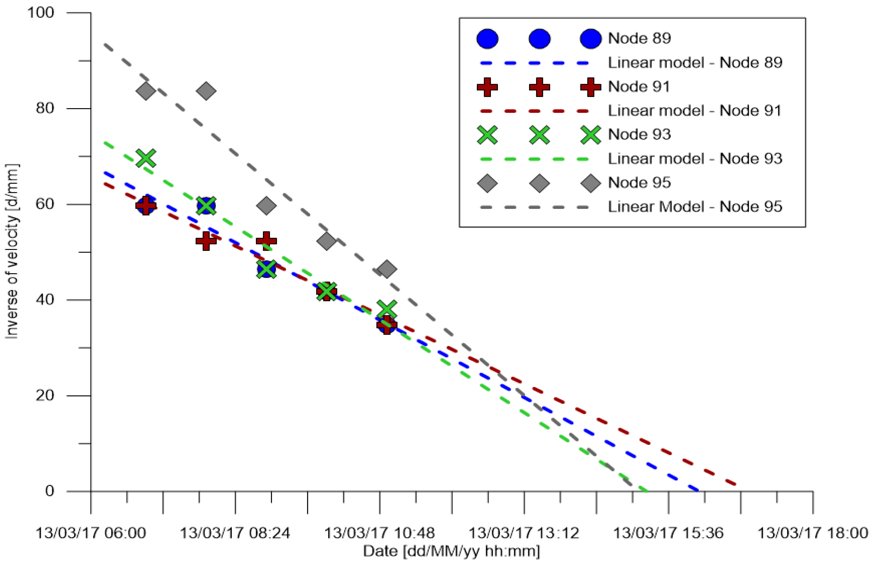
The failure event occurred on March 13 is identified by four sensors placed at 3.9, 3.2, 2.5, and 1.8 m depth (Links 89, 91, 93, and 95, respectively), with a dataset of five points each. Node 89 was correctly detected also by the activation criterion, and the time prediction was exactly the same. The back-analysis also evidenced some interesting results provided by links 91, 93, and 95. Node 91 shows a forecasting error of 2 h, while links 93 and 95 estimates the time of failure with an error of just 18 min and 10 min, respectively, with a warning time of 3 h (8 in case of real-time data transmission). As for the event that occurred on March 08, a collapse is expected in a time window that, in this case, ranges between 15:00 and 17:00 (Figure 14) (collapse observed on site between 13:56 and 14:56).
Table 4 reports the comparison of time of failure evaluation regarding the March 08 event. It can be noted that node 93 was activated by both methods, with a back-analysis estimation that starts 5 h in advance, resulting in a more complete dataset. Analysis of node 95 made with the algorithm presents a forecasting error of only 1 h, which further improves with spreadsheet back-analysis up to 15 min in advance, thanks to the improved dataset considered for the elaboration. The minimum dataset condition (five points are required to activate the time of failure estimation) caused a 1 h delay in the first application of the Fukuzono method [20]. Finally, node 99 is not considered by the software.
Table 5 reports the comparison of time of failure evaluation regarding the final collapse occurred on March 13. Node 89 was activated in the same way with both methods. This information confirms the validity of “conditioned alarm” concept, together with the IVM activation criterion hypothesis. The back-analysis includes also links 91, 93, and 95, which were not taken into consideration by the automatic algorithm. Notably, displacement occurred on March 13 is too rapid if related to the sampling period to satisfy the proposed model activation hypothesis.
4. Conclusions
The case study presented in this paper constitutes the first application of the MUMS early warning system procedure, featuring a synergic interaction between dedicated automatic activation criterion and a failure forecasting method. In particular, the algorithm developed and presented aims to substitute the manual check for a preliminary analysis and alert procedure, which could be especially useful if applied to the real-time monitoring of several landslides.
In this particular case, the automatic routine successfully identified two events thanks to the elaboration of displacement data, and related alert procedures were accordingly activated by the software. The proposed EWS allowed the occurrence of these critical events to be correctly reported, identifying the displacement rate variation and applying the failure forecast procedure to the dataset. After on-site inspection, the predictions proved correct with only some minor inaccuracies related to the exact time of collapse, with a mean value of one hour. The accelerating trend detection allowed alert messages to be sent to those responsible of monitoring, with information regarding the slope behaviour and the predicted time of failure.
Even considering the minor inaccuracies in the collapse prevision, the presented application should be considered as a positive result, bearing in mind the warning significance of the proposed method. Following these results, a back-analysis was performed through a spreadsheet software in order to identify the best outcomes achievable from available monitoring data. This analysis confirmed the results derived from the automatic algorithm application, allowing us also to improve the evaluation of the date and hour of collapse by expanding some of the datasets considered by the forecasting method. The comparison between these approaches could play a major role in the upgrading of the automatic routine, with particular attention to the main procedure developed to define the monitoring dataset to be analysed by the prevision model. In particular, some improvements could be made regarding the implementation of a real-time procedure to send monitoring data as soon as they are recorded by the instrumentation, thus overcoming the “near real-time” aspect of this application, and the possibility to further intensify the monitoring activity by increasing the sampling frequency when a possible critical event is detected.
Author Contributions
Conceptualization, A.C. and A.V.; Methodology, A.C. and A.V.; Software, A.C. and A.V.; Validation, A.C. and A.V.; Formal Analysis, A.C. and A.V.; Investigation, M.M.; Resources, M.M.; Data Curation, A.C. and M.M.; Writing-Original Draft Preparation, A.C. and A.V.; Writing-Review & Editing, A.C., A.V. and A.S.; Visualization, A.C. and A.V.; Supervision, A.S.; Project Administration, A.S. and M.M.
Funding
This research received no external funding.
Conflicts of Interest
The authors declare no conflict of interest.
References
- Greco, R.; Pagano, L. Basic features of the predictive tools of early warning systems for water-related natural hazards: Examples for shallow landslides. Nat. Hazards Earth Syst. Sci. 2017, 17, 2213–2227. [Google Scholar] [CrossRef]
- Medina-Cetina, Z.; Nadim, F. Stochastic design of an early warning system. Georisk Assess. Manag. Risk Eng. Syst. Geohazards 2008, 2, 223–236. [Google Scholar] [CrossRef]
- UN-ISDR Developing early warning systems, a checklist: Third international conference on early warning (EWC III), 27–29 March 2006, Bonn, Germany-UNISDR. Available online: https://www.unisdr.org/we/inform/publications/608 (accessed on 17 December 2018).
- Di Biagio, E.; Kjekstad, O. Early Warning, Instrumentation and Monitoring Landslides. In Proceedings of the 2nd Regional Training Course, RECLAIM II, Phuket, Thailand, 29 January–2 February 2007. [Google Scholar]
- Intrieri, E.; Gigli, G.; Mugnai, F.; Fanti, R.; Casagli, N. Design and implementation of a landslide early warning system. Eng. Geol. 2012, 147–148, 124–136. [Google Scholar] [CrossRef]
- Calvello, M.; Piciullo, L. Assessing the performance of regional landslide early warning models: The EDuMaP method. Nat. Hazards Earth Syst. Sci. 2016, 16, 103–122. [Google Scholar] [CrossRef]
- Bhasin, R.; Cepeda, J.; Lacasse, S. Experiences from cost-effective instrumentation for early warning systems installed in some hot-spot areas in South and South East Asian Countries. In Proceedings of the Second JTC1 Workshop on Triggering and Propagation of Rapid Flow-like Landslides, Hong Kong, China, 3–5 December 2018. [Google Scholar]
- Michoud, C.; Bazin, S.; Blikra, L.H.; Derron, M.-H.; Jaboyedoff, M. Experiences from site-specific landslide early warning systems. Nat. Hazards Earth Syst. Sci. 2013, 13, 2659–2673. [Google Scholar] [CrossRef] [Green Version]
- Carlà, T.; Intrieri, E.; Di Traglia, F.; Nolesini, T.; Gigli, G.; Casagli, N. Guidelines on the use of inverse velocity method as a tool for setting alarm thresholds and forecasting landslides and structure collapses. Landslides 2017, 14, 517–534. [Google Scholar] [CrossRef]
- Segalini, A.; Valletta, A.; Carri, A. Landslide time-of-failure forecast and alert threshold assessment: A generalized criterion. Eng. Geol. 2018, 245, 72–80. [Google Scholar] [CrossRef]
- Huggel, C.; Khabarov, N.; Obersteiner, M.; Ramírez, J.M. Implementation and integrated numerical modeling of a landslide early warning system: A pilot study in Colombia. Nat. Hazards 2010, 52, 501–518. [Google Scholar] [CrossRef]
- Yin, Y.; Wang, H.; Gao, Y.; Li, X. Real-time monitoring and early warning of landslides at relocated Wushan Town, the Three Gorges Reservoir, China. Landslides 2010, 7, 339–349. [Google Scholar] [CrossRef]
- Stähli, M.; Sättele, M.; Huggel, C.; McArdell, B.W.; Lehmann, P.; Van Herwijnen, A.; Berne, A.; Schleiss, M.; Ferrari, A.; Kos, A.; et al. Monitoring and prediction in early warning systems for rapid mass movements. Nat. Hazards Earth Syst. Sci. 2015, 15, 905–917. [Google Scholar] [CrossRef] [Green Version]
- Sättele, M.; Krautblatter, M.; Bründl, M.; Straub, D. Forecasting rock slope failure: How reliable and effective are warning systems? Landslides 2016, 13, 737–750. [Google Scholar] [CrossRef]
- Pecoraro, G.; Calvello, M.; Piciullo, L. Monitoring strategies for local landslide early warning systems. Available online: https://link.springer.com/article/10.1007/s10346-018-1068-z (accessed on 26 January 2019).
- Fondovalle Sangro: D’Alfonso, ecco progetto definitivo. Available online: https://www.stradeeautostrade.it (accessed on 19 December 2018).
- Piano di utilizzo terre e rocce S.S. 652 “Fondovalle Sangro” Lavori di costruzione del tratto compreso tra la stazione di Gamberale e la stazione di Civitaluparella 2° lotto –2° stralcio –2° tratto. Available online: https://sra.regione.abruzzo.it/ (accessed on 19 December 2018).
- Segalini, A.; Carini, C. Underground Landslide Displacement Monitoring: A New MMES Based Device. In Landslide Science and Practice: Volume 2: Early Warning, Instrumentation and Monitoring; Margottini, C., Canuti, P., Sassa, K., Eds.; Springer: Berlin/Heidelberg, Germany, 2013; pp. 87–93. ISBN 978-3-642-31445-2. [Google Scholar]
- Segalini, A.; Chiapponi, L.; Pastarini, B.; Carini, C. Automated Inclinometer Monitoring Based on Micro Electro-Mechanical System Technology: Applications and Verification. In Landslide Science for Safer Geoenvironment; Sassa, K., Canuti, P., Yin, Y., Eds.; Springer: Cham, Switzerland; pp. 595–600. ISBN 978-3-319-05050-8.
- Fukuzono, T. A new method for predicting the failure time of a slope. In Proceedings of the 4th International Conference and Field Workshop on Landslides, Tokyo, Japan, 23–31 August 1985; Japan Landslide Society: Tokyo, Japan, 1985; pp. 145–150. [Google Scholar]
- Petley, D.N. The evolution of slope failures: Mechanisms of rupture propagation. Nat. Hazards Earth Syst. Sci. 2004, 4, 147–152. [Google Scholar] [CrossRef]
- Rose, N.D.; Hungr, O. Forecasting potential rock slope failure in open pit mines using the inverse-velocity method. Int. J. Rock Mech. Min. Sci. 2007, 44, 308–320. [Google Scholar] [CrossRef]
- Gigli, G.; Fanti, R.; Canuti, P.; Casagli, N. Integration of advanced monitoring and numerical modeling techniques for the complete risk scenario analysis of rockslides: The case of Mt. Beni (Florence, Italy). Eng. Geol. 2011, 120, 48–59. [Google Scholar] [CrossRef]
- Mazzanti, P.; Bozzano, F.; Cipriani, I.; Prestininzi, A. New insights into the temporal prediction of landslides by a terrestrial SAR interferometry monitoring case study. Landslides 2015, 12, 55–68. [Google Scholar] [CrossRef]
Figure 1.
Case study location (Source: Bing Maps).
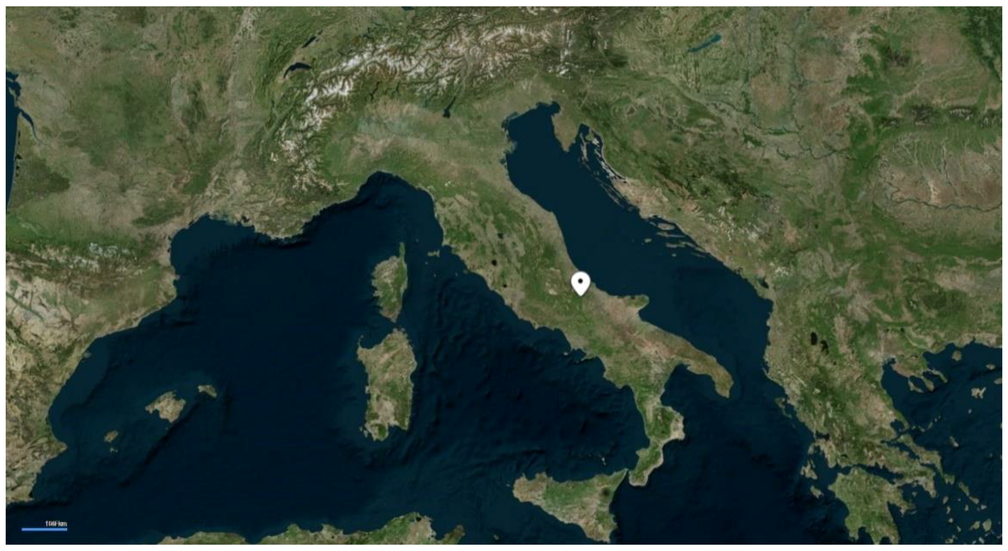
Figure 2.
Local displacements versus time starting from 5.65 m depth for (a) the whole period of monitoring and (b) starting from January 15, 2017.
Figure 2.
Local displacements versus time starting from 5.65 m depth for (a) the whole period of monitoring and (b) starting from January 15, 2017.
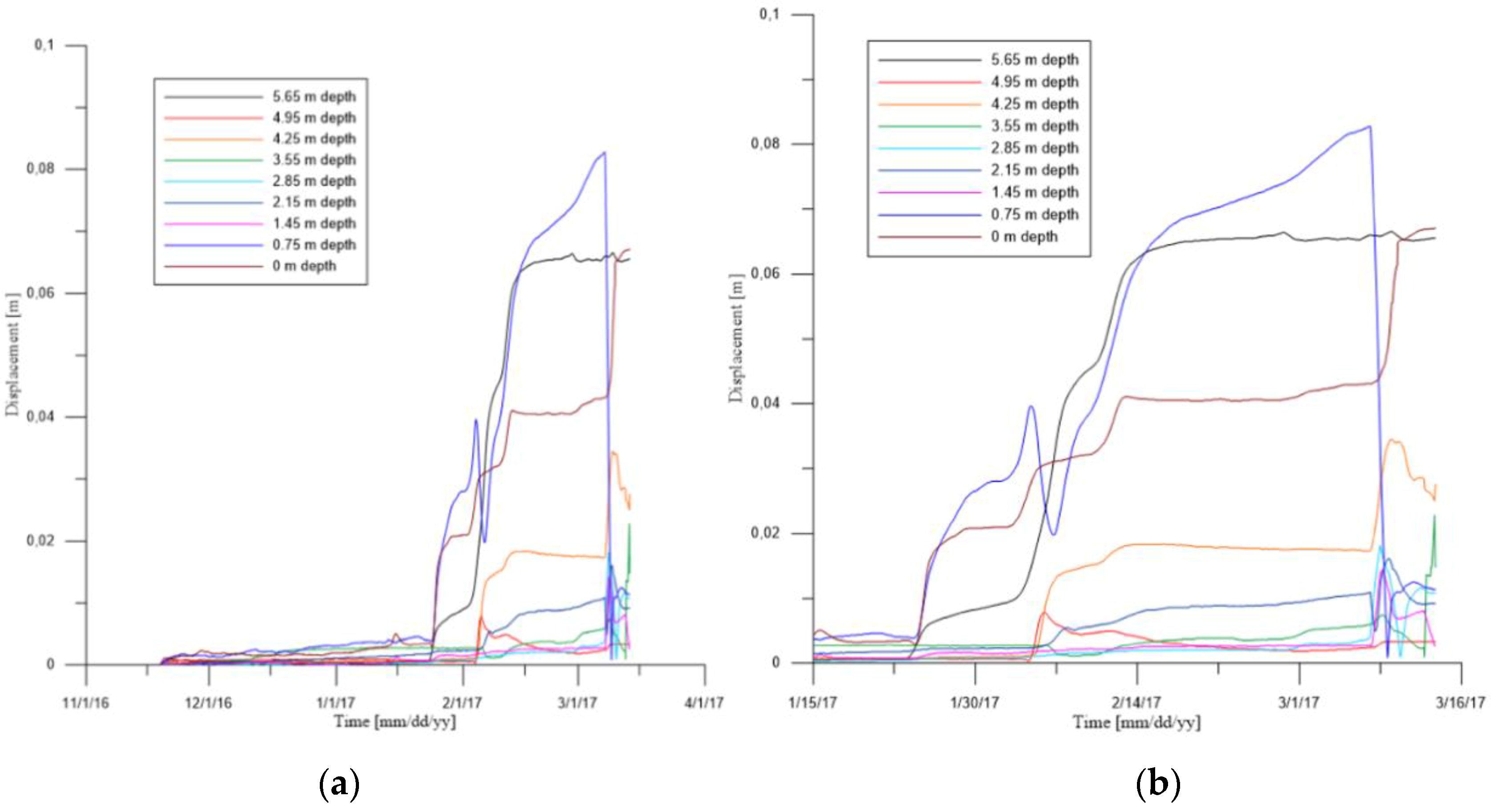
Figure 3.
(a) Displacement rates and (b) accelerations versus time starting from 5.65 m depth recorded after January 15, 2017.
Figure 3.
(a) Displacement rates and (b) accelerations versus time starting from 5.65 m depth recorded after January 15, 2017.

Figure 4.
(a) Local and (b) cumulative displacements recorded by DT0014 inclinometer at the end of the monitoring activity.
Figure 4.
(a) Local and (b) cumulative displacements recorded by DT0014 inclinometer at the end of the monitoring activity.

Figure 5.
Area surrounding MUMS vertical array as observed during on-site inspection.
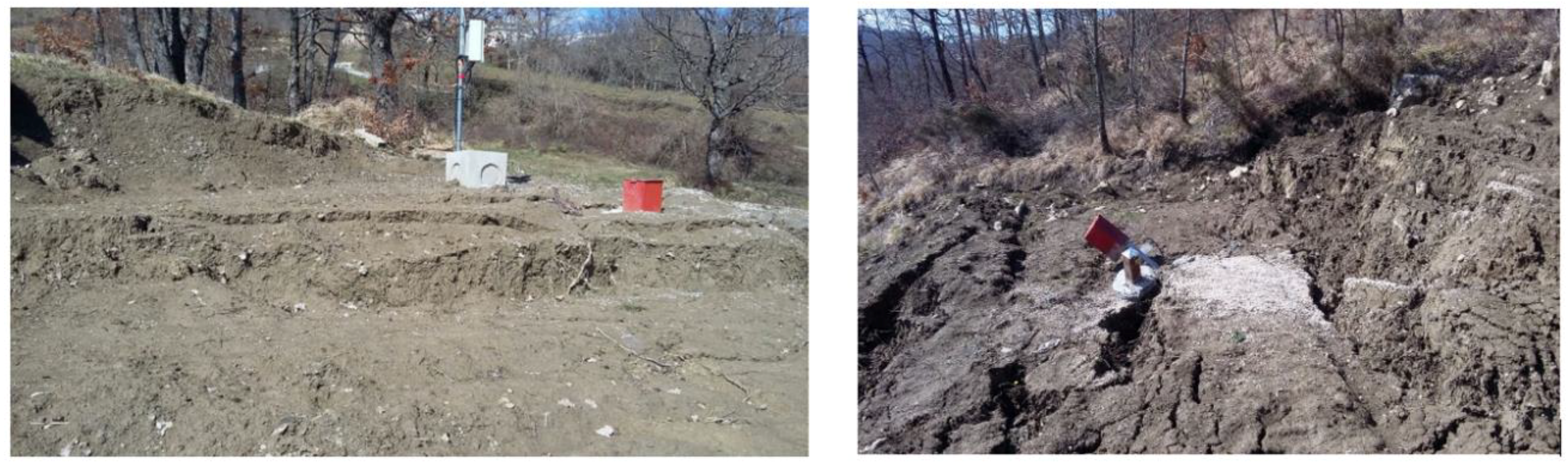
Figure 6.
(a) Inverse velocity vs time and (b) velocity vs time for cumulative displacements of node 93 with acceleration date on March 08, 2017 02:28 and time of failure forecasted on March 09, 2017 00:55.
Figure 6.
(a) Inverse velocity vs time and (b) velocity vs time for cumulative displacements of node 93 with acceleration date on March 08, 2017 02:28 and time of failure forecasted on March 09, 2017 00:55.
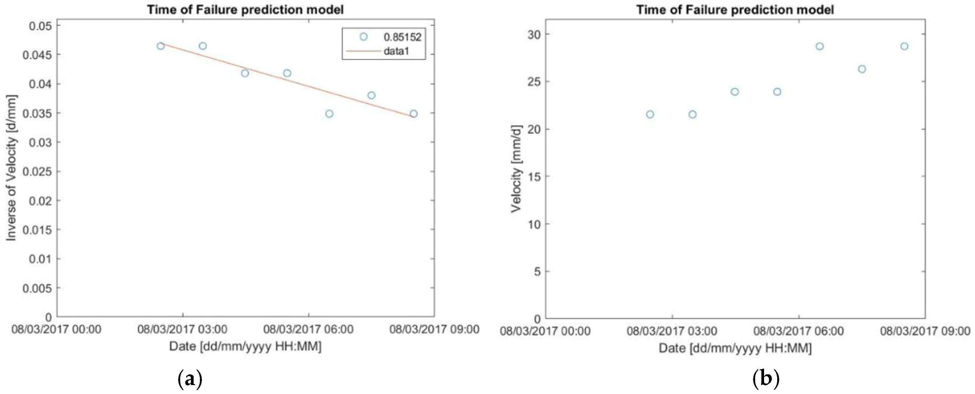
Figure 7.
(a) Inverse velocity vs time and (b) velocity vs time for cumulative displacements of node 95 with acceleration date on March 08, 2017 02:28 and time of failure forecasted on March 08, 2017 22:48.
Figure 7.
(a) Inverse velocity vs time and (b) velocity vs time for cumulative displacements of node 95 with acceleration date on March 08, 2017 02:28 and time of failure forecasted on March 08, 2017 22:48.
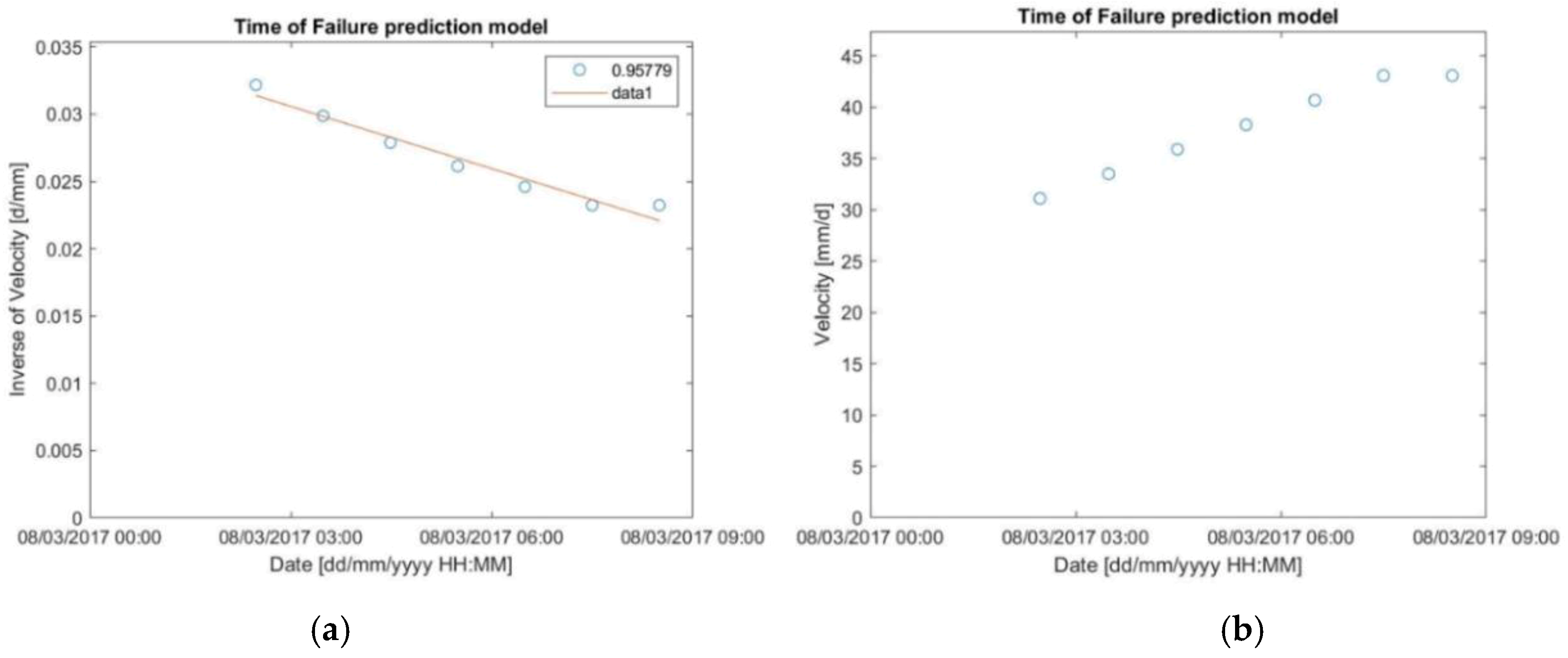
Figure 8.
(a) Inverse velocity vs time and (b) velocity vs time for local displacements of node 99 with acceleration date on March 08, 2017 21:32 and time of failure forecasted on March 09, 2017 23:59.
Figure 8.
(a) Inverse velocity vs time and (b) velocity vs time for local displacements of node 99 with acceleration date on March 08, 2017 21:32 and time of failure forecasted on March 09, 2017 23:59.

Figure 9.
(a) Inverse velocity vs time and (b) velocity vs time for local displacements of node 99 with acceleration date on March 09, 2017 05:34 and time of failure forecasted on March 09, 2017 16:48.
Figure 9.
(a) Inverse velocity vs time and (b) velocity vs time for local displacements of node 99 with acceleration date on March 09, 2017 05:34 and time of failure forecasted on March 09, 2017 16:48.
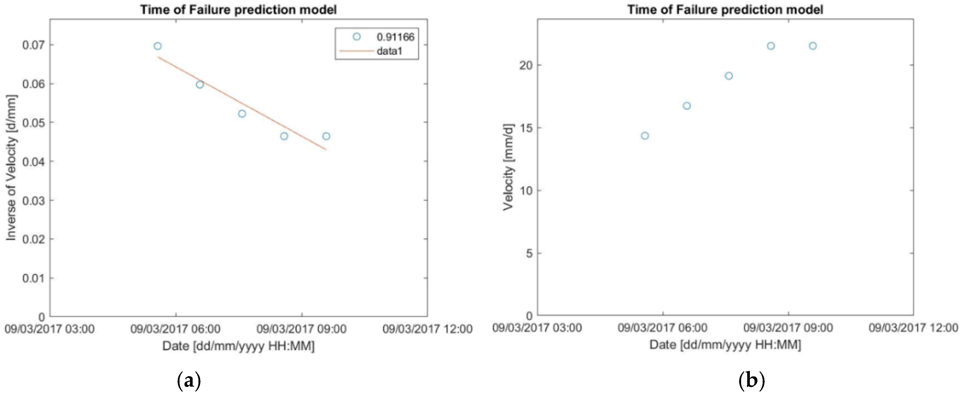
Figure 10.
(a) Inverse velocity vs time and (b) velocity vs time for cumulative displacements of node 91 with acceleration date on March 09, 2017 23:38 and time of failure forecasted on March 10, 2017 12:05.
Figure 10.
(a) Inverse velocity vs time and (b) velocity vs time for cumulative displacements of node 91 with acceleration date on March 09, 2017 23:38 and time of failure forecasted on March 10, 2017 12:05.

Figure 11.
(a) Inverse velocity vs time and (b) velocity vs time for cumulative displacements of node 89 with acceleration date on March 13, 2017 06:54 and time of failure forecasted on March 13, 2017 16:06.
Figure 11.
(a) Inverse velocity vs time and (b) velocity vs time for cumulative displacements of node 89 with acceleration date on March 13, 2017 06:54 and time of failure forecasted on March 13, 2017 16:06.
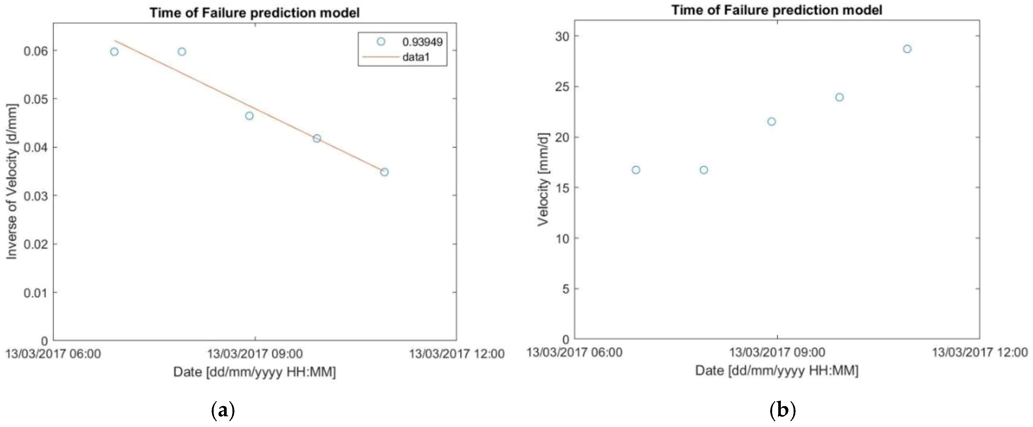
Figure 12.
Flowchart summarizing the back-analysis procedure.
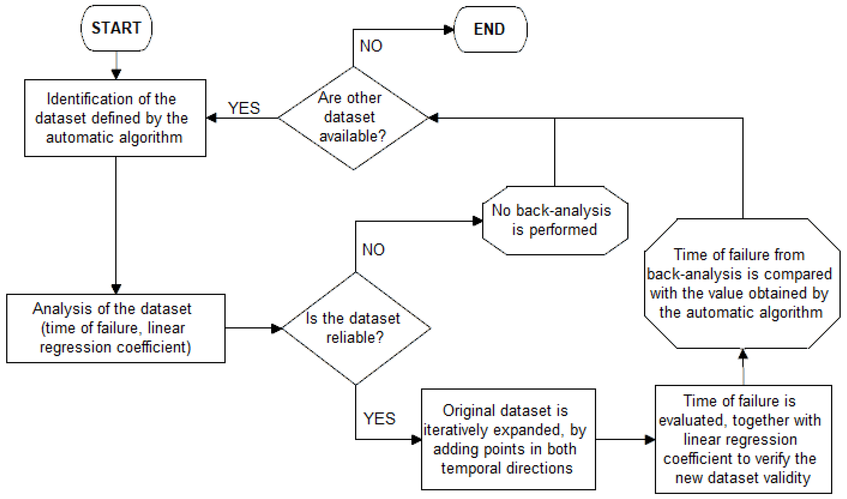
Figure 13.
Time of failure back-analysis evaluation for the event occurred on March 08, 2017.

Figure 14.
Time of failure back-analysis evaluation for the event that occurred on March 13, 2017.


Table 1.
Modular underground monitoring system (MUMS) inclinometers installed on-site at December 2018.
Table 1.
Modular underground monitoring system (MUMS) inclinometers installed on-site at December 2018.
| ID | DT0014 | DT0065 | DT0094 | DT0095 | DT0096 | DT0097 |
|---|---|---|---|---|---|---|
| Installation date | 18/11/2016 | 07/09/2017 | 19/09/2018 | 18/09/2018 | 20/09/2018 | 19/09/2018 |
| Reference reading | 19/11/2016 | 09/09/2017 | 22/09/2018 | 22/09/2018 | 22/09/2018 | 22/09/2018 |
| End of monitoring | 13/03/2017 | Ongoing | Ongoing | Ongoing | Ongoing | Ongoing |
| Array typology | Vertical Array | Vertical Array | Vertical Array | Vertical Array | Vertical Array | Vertical Array |
| Length [m] | 35 | 35 | 69 | 95 | 111 | 66 |
| Sensors typology | Tilt Link HR 3D V | Tilt Link HR 3D V | Tilt Link HR 3D V | Tilt Link HR 3D V | Tilt Link HR 3D V | Tilt Link HR 3D V |
| Number of sensors [-] | 50 | 48 | 34 | 47 | 55 | 33 |
| Interspace between sensors [m] | 0.70 | 0.70 | 2.00 | 2.00 | 2.00 | 2.00 |
Table 2.
Comparison between predicted (by the automatic algorithm) and observed Tf, together with related warning times.
Table 2.
Comparison between predicted (by the automatic algorithm) and observed Tf, together with related warning times.
| Node | Depth [m] | Onset of Acceleration [dd/MM/yy hh:mm] | Prediction [dd/MM/yyyy hh:mm] | Observed [dd/MM/yyyy hh:mm] | Forecasting Error | Theoretical Warning Time [h] | Observed Warning Time [h] |
|---|---|---|---|---|---|---|---|
| 93 | 2.5 | 08/03/2017 02:28 | 09/03/2017 00:55 | 08/03/2017 21:32 | 3 h later | 13 (22*) | 10 (19*) |
| 95 | 1.8 | 08/03/2017 02:28 | 08/03/2017 22:48 | 08/03/2017 21:32 | 1 h later | 11 (20*) | 10 (19*) |
| 99 | 0.4 | 08/03/2017 21:32 | 09/03/2017 23:59 | 08/03/2017 21:32 | postponed of 1 day and 2 h | 12 (26*) | −14 (0*) |
| 99 | 0.4 | 09/03/2017 05:34 | 09/03/2017 16:48 | 08/03/2017 21:32 | postponed of 19 h | 5 (11*) | −14 (−8*) |
| 91 | 3.2 | 09/03/2017 23:38 | 10/03/2017 12:05 | ? | not clear | 0 (12*) | ? |
| 89 | 3.9 | 13/03/2017 06:54 | 13/03/2017 16:06 | 13/03/2017 14:56 | 1.5 h later | 4 (9*) | 3 (8*) |
* value that indicates the warning time if the data transmissions were in real-time. “?” indicates uncertainty concerning the event to which the forecasting result refers.
Table 3.
Comparison between Tf predicted with the back-analysis spreadsheet and observed on-site, with related warning time.
Table 3.
Comparison between Tf predicted with the back-analysis spreadsheet and observed on-site, with related warning time.
| Node | Depth [m] | Acceleration Date [dd/MM/yyyy hh:mm] | Prediction [dd/MM/yyyy hh:mm] | Observed [dd/MM/yyyy hh:mm] | Forecasting Error | Theoretical Warning Time [h] | Observed Warning Time [h] |
|---|---|---|---|---|---|---|---|
| 93 | 2.5 | 07/03/2017 20:27 | 08/03/2017 20:54 | 08/03/2017 21:32 | 38 min in advance | 9 (24.5*) | 9 (25*) |
| 95 | 1.8 | 08/03/2017 01:28 | 08/03/2017 21:17 | 08/03/2017 21:32 | 15 min in advance | 9 (20*) | 9 (20*) |
| 99 | 0.0 | 08/03/2017 11:30 | 08/03/2017 21:13 | 08/03/2017 21:32 | 19 min in advance | 9 (10*) | 9 (10*) |
| 89 | 3.9 | 13/03/2017 06:54 | 13/03/2017 16:06 | 13/03/2017 14:56 | 1.5 h later | 4 (9*) | 3 (8*) |
| 91 | 3.2 | 13/03/2017 06:54 | 13/03/2017 16:56 | 13/03/2017 14:56 | 2 h later | 5 (10*) | 3 (8*) |
| 93 | 2.5 | 13/03/2017 06:54 | 13/03/2017 15:14 | 13/03/2017 14:56 | 18 min later | 3 (8*) | 3 (8*) |
| 95 | 1.8 | 13/03/2017 06:54 | 13/03/2017 15:06 | 13/03/2017 14:56 | 10 min later | 3 (8*) | 3 (8*) |
* warning time if the data transmissions were in real-time.
Table 4.
Comparison between algorithm and spreadsheet Tf analysis of the event occurred on March 08, 2017.
Table 4.
Comparison between algorithm and spreadsheet Tf analysis of the event occurred on March 08, 2017.
| Node | Analysis | Acceleration Date [dd/MM/yyyy hh:mm] | Prediction [dd/MM/yyyy hh:mm] | Observed [dd/MM/yyyy hh:mm] | Forecasting Error | Theoretical Warning Time [h] | Observed Warning Time [h] |
|---|---|---|---|---|---|---|---|
| 93 | Back -analysis | 07/03/2017 20:27 | 08/03/2017 20:54 | 08/03/2017 21:32 | 38 min in advance | 9 (24.5*) | 9 (25*) |
| 95 | Back-analysis | 08/03/2017 01:28 | 08/03/2017 21:17 | 08/03/2017 21:32 | 15 min in advance | 9 (20*) | 9 (20*) |
| 93 | Algorithm | 08/03/2017 02:28 | 09/03/2017 00:55 | 08/03/2017 21:32 | 3 h later | 13 (22*) | 10 (19*) |
| 95 | Algorithm | 08/03/2017 02:28 | 08/03/2017 22:48 | 08/03/2017 21:32 | 1 h later | 11 (20*) | 10 (19*) |
| 99 | Back-analysis | 08/03/2017 11:30 | 08/03/2017 21:13 | 08/03/2017 21:32 | 19 min in advance | 9 (10*) | 9 (10*) |
* warning time if the data transmissions were in real-time.
Table 5.
Comparison between algorithm and spreadsheet Tf analysis of the event occurred on March 13, 2017.
Table 5.
Comparison between algorithm and spreadsheet Tf analysis of the event occurred on March 13, 2017.
| Node | Analysis | Acceleration Date [dd/MM/yy hh:mm] | Prediction [dd/MM/yyyy hh:mm] | Observed [dd/MM/yyyy hh:mm] | Forecasting Error | Theoretical Warning Time [h] | Observed Warning Time [h] |
|---|---|---|---|---|---|---|---|
| 89 | Back-analysis | 13/03/2017 06:54 | 13/03/2017 16:06 | 13/03/2017 14:56 | 1.5 h later | 4 (9*) | 3 (8*) |
| 89 | Algorithm | 13/03/2017 06:54 | 13/03/2017 16:06 | 13/03/2017 14:56 | 1.5 h later | 4 (9*) | 3 (8*) |
| 91 | Back-analysis | 13/03/2017 06:54 | 13/03/2017 16:56 | 13/03/2017 14:56 | 2 h later | 5 (10*) | 3 (8*) |
| 93 | Back-analysis | 13/03/2017 06:54 | 13/03/2017 15:14 | 13/03/2017 14:56 | 18 min later | 3 (8*) | 3 (8*) |
| 95 | Back-analysis | 13/03/2017 06:54 | 13/03/2017 15:06 | 13/03/2017 14:56 | 10 min later | 3 (8*) | 3 (8*) |
* warning time if the data transmissions were in real-time.
© 2019 by the authors. Licensee MDPI, Basel, Switzerland. This article is an open access article distributed under the terms and conditions of the Creative Commons Attribution (CC BY) license (http://creativecommons.org/licenses/by/4.0/).
Share and Cite
MDPI and ACS Style
Segalini, A.; Carri, A.; Valletta, A.; Martino, M. Innovative Monitoring Tools and Early Warning Systems for Risk Management: A Case Study. Geosciences 2019, 9, 62. https://doi.org/10.3390/geosciences9020062
AMA Style
Segalini A, Carri A, Valletta A, Martino M. Innovative Monitoring Tools and Early Warning Systems for Risk Management: A Case Study. Geosciences. 2019; 9(2):62. https://doi.org/10.3390/geosciences9020062
Chicago/Turabian StyleSegalini, Andrea, Andrea Carri, Alessandro Valletta, and Maurizio Martino. 2019. "Innovative Monitoring Tools and Early Warning Systems for Risk Management: A Case Study" Geosciences 9, no. 2: 62. https://doi.org/10.3390/geosciences9020062
Note that from the first issue of 2016, this journal uses article numbers instead of page numbers. See further details here.